A Convex Model for Edge-Histogram Specification with Applications to Edge-Preserving Smoothing

1
Department of Mathematics, The Chinese University of Hong Kong, Hong Kong
2
Centre de Mathématiques et de Leurs Applications, ENS de Cachan, 94230 Paris, France
*
Author to whom correspondence should be addressed.
Axioms 2018, 7(3), 53; https://doi.org/10.3390/axioms7030053
Submission received: 18 June 2018
/
Revised: 1 August 2018
/
Accepted: 1 August 2018
/
Published: 2 August 2018
(This article belongs to the Special Issue Advanced Numerical Methods in Applied Sciences)
Abstract
:The goal of edge-histogram specification is to find an image whose edge image has a histogram that matches a given edge-histogram as much as possible. Mignotte has proposed a non-convex model for the problem in 2012. In his work, edge magnitudes of an input image are first modified by histogram specification to match the given edge-histogram. Then, a non-convex model is minimized to find an output image whose edge-histogram matches the modified edge-histogram. The non-convexity of the model hinders the computations and the inclusion of useful constraints such as the dynamic range constraint. In this paper, instead of considering edge magnitudes, we directly consider the image gradients and propose a convex model based on them. Furthermore, we include additional constraints in our model based on different applications. The convexity of our model allows us to compute the output image efficiently using either Alternating Direction Method of Multipliers or Fast Iterative Shrinkage-Thresholding Algorithm. We consider several applications in edge-preserving smoothing including image abstraction, edge extraction, details exaggeration, and documents scan-through removal. Numerical results are given to illustrate that our method successfully produces decent results efficiently.
1. Introduction
Histogram specification is a process where the image histogram is altered such that the histogram of the output image follows a prescribed distribution. It is one of the many important tools in image processing with numerous applications such as image enhancement [1,2,3], segmentation [4,5,6] among many others. To match the histogram of an image I to a target histogram , one can use the following procedure:
- Compute the probability density function of I, , , where denotes the intensity values, denotes the number of pixels whose value equals to , and n is the total number of pixels in I.
- With the probability density function , compute the cumulative density function of I.
- With serving as a probability density function, compute the cumulative density function .
- For , replace by , where .
In the typical 8-bit image setting, and , for .
However, the above procedure gives an inexact histogram matching in discrete images, since the number of pixels is far greater than the number of intensity values in discrete images. Therefore, to ensure exact matching of histograms, different algorithms are introduced, see for instance [7,8,9]. The main idea of these algorithms is to obtain a total order of the pixel values before setting pixel values according to the target histogram.
The goal of edge-histogram specification is to find an image whose edge image has a histogram that matches a given edge-histogram as much as possible. An edge-histogram of an image counts the frequencies of different gradient values in an image and plots the distribution of gradient values. Edge-histograms of natural images have been studied in previous literature [10,11]. It is known that the edge-histograms of natural images contain a sharp peak at 0. This phenomenon is due to the abundance of flat regions in natural images. In natural images, flat regions are seen in the sky, water, walls, and many others. The flat regions in the image produce zero gradients and hence the resulting edge-histogram contains a sharp peak at 0. In addition, as stated in [10], the edge-histograms of natural images have a higher kurtosis and heavier tails compared to a Gaussian distribution with the same mean and variance.
Histogram of gradients has also been used in other fields of image processing. Histogram of oriented gradients (HOG) is used as a feature descriptor for object detection [12,13,14]. This technique first counts the frequencies of gradient orientation in terms of a histogram in a local region, and combines the histograms of gradients in different regions to a single vector as output.
Unlike HOG, our focus is on matching edge-histograms, and we do not consider local edge-histograms. To match the edge-histogram, the author in [11] proposed the following non-convex model for the problem. Given a discrete input image I of size m-by-n, let be a vector storing the pairwise differences
where denotes the value of the i-th pixel of I, and denotes the set of indices of a fixed shape neighborhood of the s-th pixel, for example, the north, east, south, and west neighboring points of the s-th pixel. Here with the number of elements in . That is, each entry of the vector contains the absolute difference between the values of two neighboring pixels in I. Note that the order of storing the pairwise differences does not matter, as it does not affect the output of histogram specification.
Given a target edge-histogram , one can apply histogram specification on to match . Denote the output by :
To ensure exact histogram matching, the author of [11] used the algorithm in [7]. After applying histogram specification as in (2), one gets the output image X by solving the minimization problem
Model (3) is solved by a conjugate gradient procedure followed by a stochastic local search, please refer to [7,11] for the full details of the algorithm. The non-convex nature of the model hinders the computations, and it is difficult to include additional constraints. In this paper, we propose a convex model that can include additional constraints based on different applications in edge-preserving smoothing.
Edge-preserving smoothing is a popular topic in image processing and computer graphics. Its aim is to suppress insignificant details and keep important edges intact. As an example, the input image in Figure 3a contains textures on the slate and the goal of edge-preserving smoothing is to remove such textures and keep only the object boundaries as in Figure 3c. Numerous methods have been introduced to perform the task. Anisotropic diffusion [15,16] performs smoothing by means of solving a non-linear partial differential equation. Bilateral filtering [17,18,19,20] is a method combining domain filters and range filters. They are widely used because of their simplicity. Optimization frameworks such as the weighted least squares (WLS) [21] and TV regularization [22,23] are also introduced. In WLS, a regularization term is added to minimize the horizontal and vertical gradients with corresponding smoothness weights. Recently, models based on -gradient minimization [24,25,26,27,28,29] have become popular. These models focus on the -norm of the image gradients.
One application of edge-preserving smoothing is scan-through removal. Written or printed documents are usually subjected to various degradations. In particular, two-sided documents can be suffered from the effect of back-to-front interference, known as “see-through”, see Figure 10. The problem is especially severe in old documents, which is caused by the bad quality of the paper or ink-bleeding. These effects greatly reduce the readability and hinder optical character recognition. Therefore it is of great importance to remove such interference. However, physical restoration is difficult as it may damage the original contents of the documents, which is clearly undesirable as the contents may be important. Consequently, different approaches in the field of image processing are considered to restore the images digitally.
These approaches can be mainly classified into two classes: Blind and Non-blinds methods. Non-blind methods [30,31,32,33,34,35,36,37,38] require the information of both sides. These methods usually consist of two steps. First, the two sides of the images are registered. Then, the output image is computed based on the registered images. It is obvious that these methods strongly depend on the quality of registration; therefore, highly accurate registration is needed. However, perfect registration is hard to achieve in practice due to numerous sources of errors including local distortions and scanning errors. Furthermore, information from the back page is not available on some occasions. Therefore, blind methods which do not assume the availability of the back page are also developed in solving the problem, see [39,40,41,42,43,44].
In this paper, we propose a convex model for applications in edge-preserving smoothing. In our work, we modify the objective function in the non-convex model in [11] so that we only need to solve a convex minimization problem to obtain the output. The simplicity of our model allows us to incorporate different useful constraints such as the dynamic range constraint; the convexity of our model allows us to compute the output efficiently by Fast Iterative Shrinkage-Thresholding Algorithm (FISTA) [45] or Alternating Direction Method of Multipliers (ADMM) [46,47]. We introduce different edge-histograms and suitable constraints in our model, and apply them to different imaging tasks in edge-preserving smoothing, including image abstraction, edge extraction, details exaggeration, and scan-through removal.
The contribution of this paper is twofold. First, we propose a convex variant of the model in [11] which can be solved efficiently. In addition, our model can easily include additional constraints based on different applications. Second, we demonstrate applications of edge-histogram specification in edge-preserving smoothing.
2. Our Model
In our model, we do not consider the edge magnitudes as in (1). Instead, we directly consider the image gradients and define with entries
Similar to [11], our model consists of two parts. First, given , we apply histogram specification on to obtain as in (2). In the second part, we solve a minimization problem to obtain the output X. Instead of solving the non-convex model (3), we propose a convex model. In Section 2.1, we present our convex model and its solvers. In Section 2.2, Section 2.3 and Section 2.4, we apply our model to specific applications in edge-preserving smoothing.
In the following discussions, we consider only grayscale images. For colored images, we apply our method to R, G, B channels separately.
2.1. Proposed Convex Model
Instead of (3), we propose the convex model
where or 2, is a convex set to be discussed in Section 2.4, and denotes the indicator function of . The choices of p and depend on the applications. Let be a vector such that its s-th entry is . Then we can rewrite (4) as
In our tests, we use , where and denote the indices of the north of north and west neighboring points of the s-th pixel respectively. Hence we can write , where , are the horizontal and vertical backward difference operators. We use periodic boundary condition for pixels outside the boundaries, see ([48], p. 258).
2.2. Construction of Target Edge-Histogram
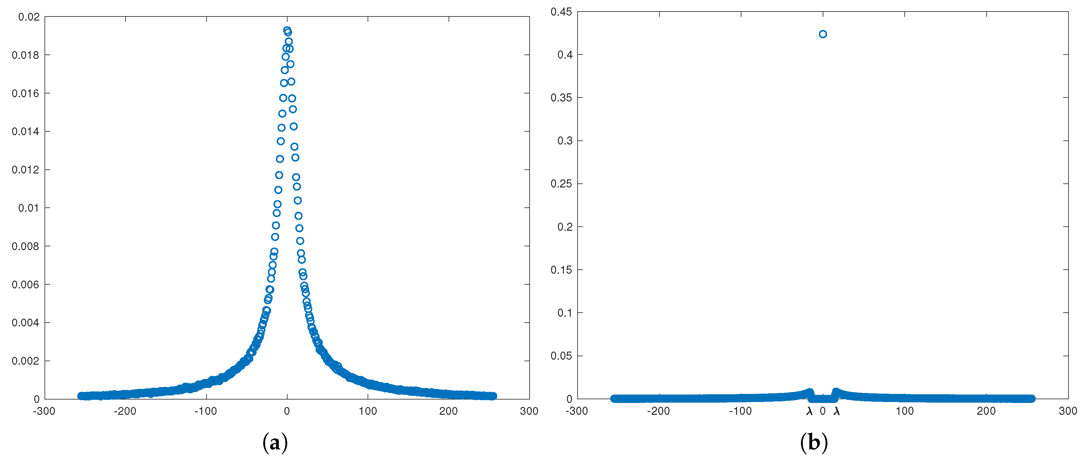
For the applications we considered in this paper, one objective is to remove textures in the images where their edges have a small magnitude. As an example, the textures on the slate in Figure 1a produce smaller edge magnitudes compared to the boundaries of the slate and the letters on the slate, see Figure 1b,c. To eliminate those textures, we could set the values of edges with a small magnitude to zero. Hence, in this paper, we propose to use edge-histograms similar to that shown in Figure 2b as target edge-histogram which is obtained by thresholding the input edge-histogram in Figure 2a. In particular, the target edge-histogram is dependent on the input image. We remark here that it is not uncommon to construct the target histogram based on the input. For example, such construction is used in image segmentation [6].
Since we are just thresholding the edges with small values to zero, the edge-histogram specification (2) can be done easily as follows. Given any input image Y, we first compute its gradients . Then we set
2.3. Gaussian Smoothing and Iterations
Strong textures produce edges with large magnitude, which cannot be eliminated using a thresholded edge-histogram as in Figure 2b. To suppress them, the input image I will first pass through a Gaussian filter with standard deviation to get the initial guess . Larger will have a greater effect in suppressing strong textures, but at the same time blur the image. Hence, should be chosen small enough so that the Gaussian-filtered image is visually equal to I. In our tests, is chosen to be less than 1. However, there is not an automatic way to compute the optimal . Hence in this model, we leave as a parameter to be chosen manually by users. Let be the Gaussian-filtered image. Whenever such suppression is unnecessary, we set and hence .
As mentioned in Section 2.2, one of our objectives is to map weak edges to zero. This can be done by changing the in the thresholded edge-histogram or by solving (5) repeatedly. More specifically, given , we construct using (6) and solve (5) to obtain . Then we repeat the process to obtain and so on. Figure 4 shows a comparison; while we see in Figure 4b that the result after one iteration still contains textures in the grasses, almost all of them are removed after three iterations, see Figure 4c.
2.4. Convex Set
The model (3) does not consider the dynamic range constraint
For example, consider the case when one defines such that every pixel of is doubled. In the absence of (7), it is easy to get an exact solution X of (3) if any one of the pixel values is given. However, there is no guarantee that the pixel values of X lie within . Therefore, when X is converted back to the desired dynamic range, either by stretching or clipping, the edge-histogram is no longer preserved. To avoid this, it is better to include the dynamic range constraint in the objective function. Therefore, we use the following constraint in all our applications:
In scan-through removal, we assume the background in books and articles have a lighter intensity than the ink in all color channels. Therefore, in addition to the dynamic range constraint, we also keep the value of the background pixels unchanged. Hence, we set
where is the approximate intensity of the background to be defined in Section 3.4.
3. Applications and Comparisons
Edge-preserving smoothing includes many different applications. In this section, we consider four applications, namely image abstraction, edge extraction, details exaggeration, and scan-through removal. For the first three applications, we use in (5) and solve it by FISTA with the input image as an initial guess. We compare with four existing methods: bilateral filtering [18], weighted-least square [21], -smoothing [24], and -projection [29]. For the scan-through removal, we use in (5) and solve it by ADMM with the input image and as the initial guesses. We compare with one blind method [43] and three non-blind methods [32,44,49]. In all applications, the number of iterations is fixed at 3. The values and vary for different images and will be stated separately.
For the tests below, we select the parameters which give the output image with the best visual quality. Some of the comparison results are obtained directly from the authors’ work and some are done by ourselves. For the results done by ourselves, we list out the parameters we have used.
3.1. Image Abstraction
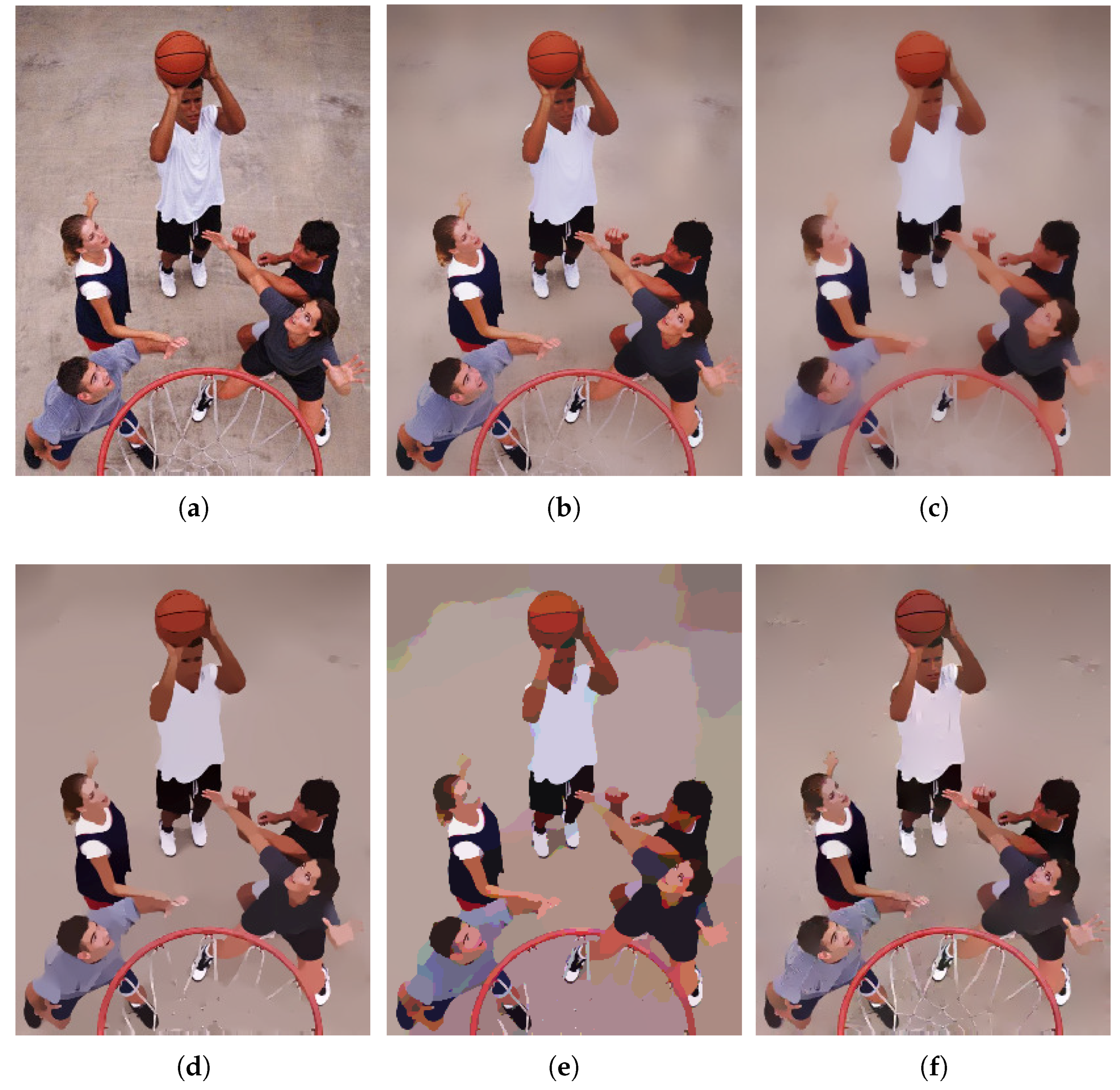
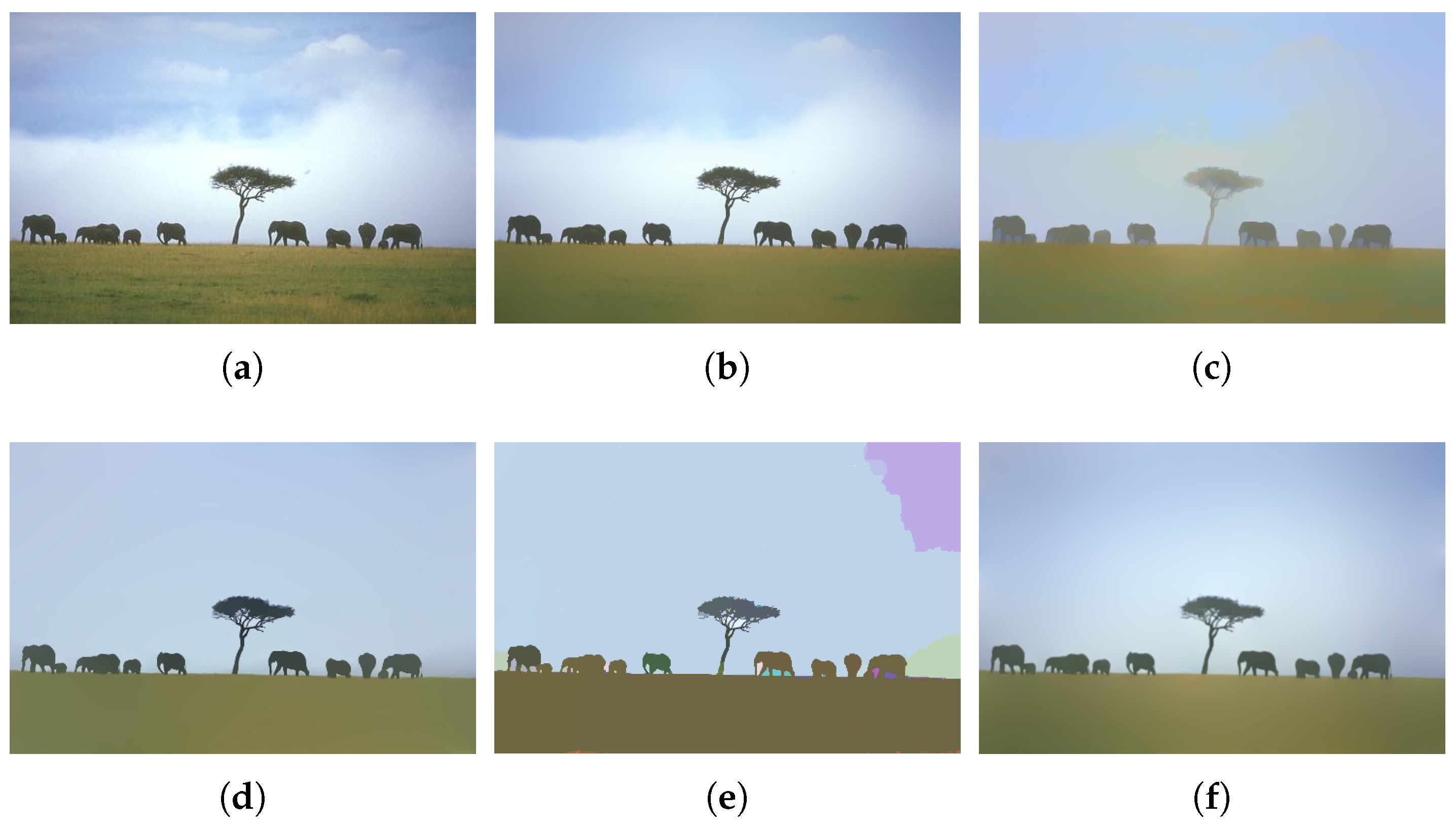
The goal of image abstraction is to remove textures and fine details so that the output looks un-photorealistic. This can be done by solving (5) with constraint (8). As shown in Figure 5, the textures of the objects in the photorealistic input image in Figure 5a is removed and our output in Figure 5f becomes un-photorealistic. We see that our model successfully eliminates almost all object textures and keeps the object boundaries intact. As we see in Figure 5f, the details in the basketball net in our output are kept intact, while it disappears, or almost disappears, in the outputs of other models.
3.2. Edge Extraction
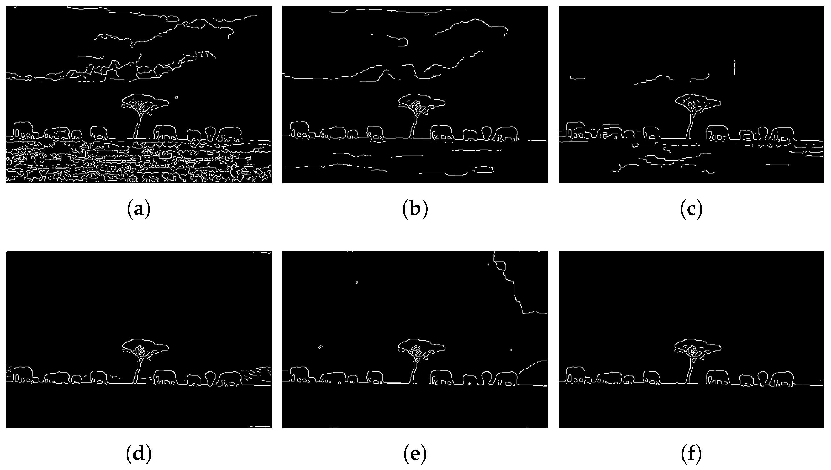
Object textures are sometimes misclassified as edges during the edge detection process. In order to reduce misclassifications, image abstraction as discussed in the last section can be used to suppress object textures. Given an input image as shown in Figure 6a, objects of less importance such as clouds and grasses can be eliminated by image abstraction. Using our method, a smooth image as in Figure 6f is obtained. Edge detection or segmentation can then be applied to the output image to obtain a result with much fewer distortions. Figure 7 shows the results of applying the Canny edge detector to the grayscale version of Figure 6. We see that while the outputs of other models keep unnecessary details, our model produces a result containing only salient edges, and removes unimportant details.
3.3. Details Exaggeration
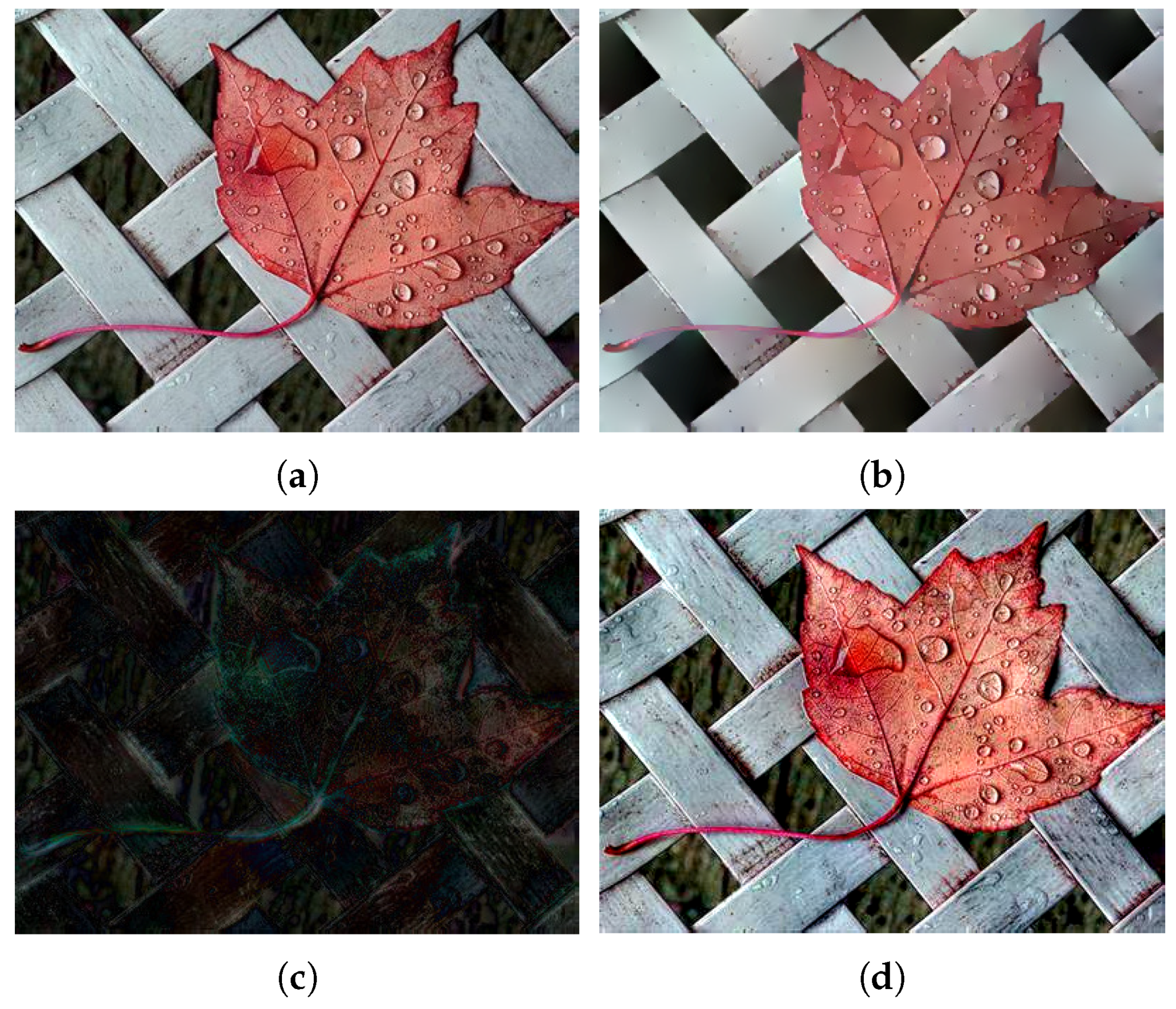
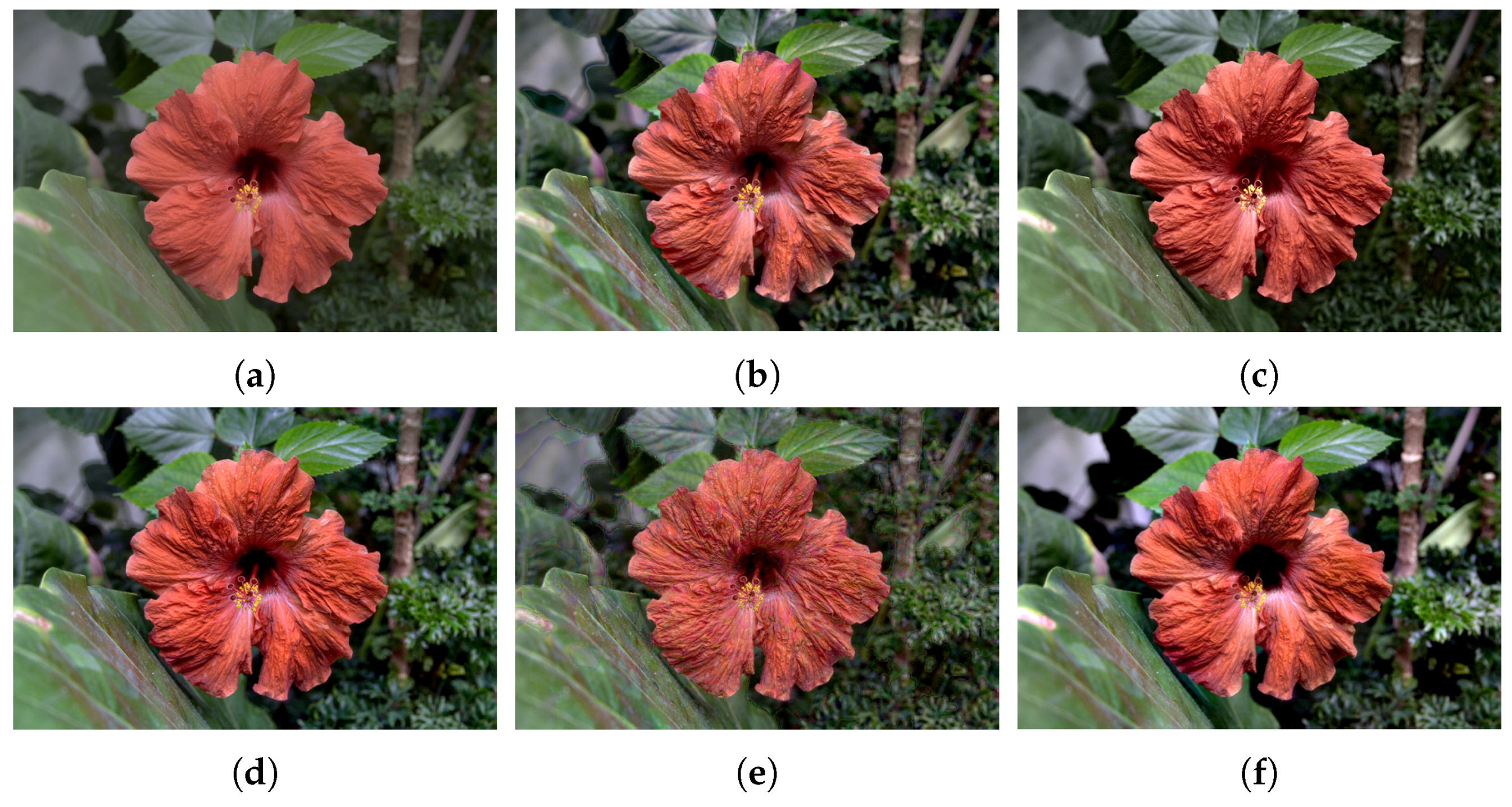
Details exaggeration is to enhance the fine details in an image as much as possible. Given an input image I, we obtain a smooth image X by our method where the textures in I are removed, see in Figure 8b. As seen in Figure 8c, the image has small values in regions with insignificant textures and large values in the parts containing strong textures. By enhancing () and adding it back to X, a details-exaggerated image J can be obtained, see Figure 8d. Mathematically, we have , where is a parameter controlling the extent of exaggeration. Figure 9 shows a comparison with the results by other methods. In Figure 9f we see that our model successfully produces a better result with more exaggerated details.
3.4. Scan-Through Removal
Two-sided documents can be suffered from the effect of back-to-front interference, known as “see-through”. Usually, “see-through” produces relatively small gradient fluctuations than the main content we want to preserve, see Figure 10. By considering the edges, one can identify interferences and eliminate them.
Recall in (9), we also impose a constraint that background pixels will not be modified. Here background pixels refer to the pixels with values not less than . To find a suitable , we first need to locate background regions—regions which contain only insignificant intensity change, i.e., the standard deviation of the intensity within the region should be small. Motivated by this, we design a multi-scale sliding window method to compute a suitable . A sliding window with size w is used to scan through an input image Y with stride . At each location p, the mean intensity of the sliding window is computed and if its standard deviation is smaller than a parameter , will be stored for future selection. After scanning through the whole image, we set to the largest stored value to avoid choosing regions with purely foreground or interference. If for all p, we replace w by and scan through the image again. At the worst case when , it is equivalent to setting to the maximum intensity of the image. In our tests, we use .
The reason for using a varying window size is that a small window will have a chance of capturing extreme values and a large window will have a chance of failing in capturing pure background. Therefore, we start from a large window and stop once we find at least one region with a small standard deviation. The initial window we use is the largest square window of length that can fit inside the given image. Figure 10 shows the windows (red-colored squares) obtained by the procedure above. We see that it successfully locates a pure background. The background level is the mean intensity of the corresponding square.
With found, we solve our model (5) with constraint (9) to obtain the output. We test our method using the first image in Figure 10. Our output is shown in Figure 11b, where we see that the contents are kept and the back-page interferences are removed. Figure 11a shows a comparison with the blind method from [43]. We also compare our result with three non-blind methods [32,44,49]. For copyright reasons, we can only refer readers to the papers [32,44] to see the resulting images from the three methods. Our method outperforms the blind method and is comparable to the non-blind methods, while these non-blind methods require information from both sides.
4. Conclusions
We have proposed a convex model with suitable constraints for edge-preserving smoothing tasks including image abstraction, edge extraction, details exaggeration, and documents scan-through removal. Our convex model allows us to solve it efficiently by existing algorithms.
In this paper, because of the special applications we considered, we use only the thresholded histograms as target edge-histograms. In the future, we would investigate more general shapes of edge-histograms and apply them to a wider class of problems.
Author Contributions
Conceptualization, K.C.K.C., R.H.C. and M.N.; Data curation, K.C.K.C. and M.N.; Formal analysis, K.C.K.C., R.H.C. and M.N.; Funding acquisition, R.H.C. and M.N.; Investigation, K.C.K.C., R.H.C. and M.N.; Methodology, K.C.K.C., R.H.C. and M.N.; Resources, K.C.K.C., R.H.C. and M.N.; Software, K.C.K.C. and M.N.; Supervision, R.H.C. and M.N.; Validation, K.C.K.C., R.H.C. and M.N.; Visualization, K.C.K.C. and R.H.C.; Writing—original draft, K.C.K.C.; Writing—review & editing, K.C.K.C. and R.H.C.
Funding
This research is supported by HKRGC Grants No. CUHK14306316, HKRGC CRF Grant C1007-15G, HKRGC AoE Grant AoE/M-05/12, CUHK DAG No. 4053211, and CUHK FIS Grant No. 1907303, and French Research Agency (ANR) under grant No ANR-14-CE27-001 (MIRIAM) and by the Isaac Newton Institute for Mathematical Sciences for support and hospitality during the programme Variational Methods and Effective Algorithms for Imaging and Vision, EPSRC grant no EP/K032208/1.
Conflicts of Interest
The authors declare no conflict of interest.
References
- Lee, S.; Tseng, C. Color image enhancement using histogram equalization method without changing hue and saturation. In Proceedings of the 2017 IEEE International Conference on Consumer Electronics-Taiwan, Taipei, Taiwan, 12–14 June 2017; pp. 305–306. [Google Scholar]
- Lim, S.; Isa, N.; Ooi, C.; Toh, K. A new histogram equalization method for digital image enhancement and brightness preservation. Signal Image Video Process. 2015, 9, 675–689. [Google Scholar] [CrossRef]
- Wang, Y.; Chen, Q.; Zhang, B. Image enhancement based on equal area dualistic sub-image histogram equalization method. IEEE Trans. Consum. Electron. 1999, 45, 68–75. [Google Scholar] [CrossRef]
- Chen, Y.; Chen, D.; Li, Y.; Chen, L. Otsu’s thresholding method based on gray level-gradient two-dimensional histogram. In Proceedings of the 2010 2nd International Asia Conference on Informatics in Control, Automation and Robotics, Wuhan, China, 6–7 March 2010; Volume 3, pp. 282–285. [Google Scholar]
- Tobias, O.; Seara, R. Image segmentation by histogram thresholding using fuzzy sets. IEEE Trans. Image Process. 2002, 11, 1457–1465. [Google Scholar] [CrossRef] [PubMed]
- Thomas, G. Image segmentation using histogram specification. In Proceedings of the 2008 15th IEEE International Conference on Image Processing, San Diego, CA, USA, 12–15 October 2008; pp. 589–592. [Google Scholar]
- Coltuc, D.; Bolon, P.; Chassery, J. Exact histogram specification. IEEE Trans. Image Process. 2006, 15, 1143–1152. [Google Scholar] [CrossRef] [PubMed]
- Sen, D.; Pal, S. Automatic exact histogram specification for contrast enhancement and visual system based quantitative evaluation. IEEE Trans. Image Process. 2011, 20, 1211–1220. [Google Scholar] [CrossRef] [PubMed]
- Nikolova, M.; Wen, Y.; Chan, R. Exact histogram specification for digital images using a variational approach. J. Math. Imaging Vis. 2013, 46, 309–325. [Google Scholar] [CrossRef]
- Zhu, S.; Mumford, D. Prior learning and Gibbs reaction-diffusion. IEEE Trans. Pattern Anal. Mach. Intell. 1997, 19, 1236–1250. [Google Scholar] [Green Version]
- Mignotte, M. An energy-based model for the image edge-histogram specification problem. IEEE Trans. Image Process. 2012, 21, 379–386. [Google Scholar] [CrossRef] [PubMed]
- Dalal, N.; Triggs, B. Histograms of oriented gradients for human detection. In Proceedings of the IEEE Computer Society Conference on Computer Vision and Pattern Recognition, San Diego, CA, USA, 20–25 June 2005; Volume 1, pp. 886–893. [Google Scholar]
- Zhu, Q.; Yeh, M.; Cheng, K.; Avidan, S. Fast human detection using a cascade of histograms of oriented gradients. In Proceedings of the IEEE Computer Society Conference on Computer Vision and Pattern Recognition, New York, NY, USA, 17–22 June 2006; Volume 2, pp. 1491–1498. [Google Scholar]
- Déniz, O.; Bueno, G.; Salido, J.; De la Torre, F. Face recognition using histograms of oriented gradients. Pattern Recognit. Lett. 2011, 32, 1598–1603. [Google Scholar] [CrossRef]
- Perona, P.; Malik, J. Scale-space and edge detection using anisotropic diffusion. IEEE Trans. Pattern Anal. Mach. Intell. 1990, 12, 629–639. [Google Scholar] [CrossRef] [Green Version]
- Black, M.; Sapiro, G.; Marimont, D.; Heeger, D. Robust anisotropic diffusion. IEEE Trans. Image Process. 1998, 7, 421–432. [Google Scholar] [CrossRef] [PubMed] [Green Version]
- Tomasi, C.; Manduchi, R. Bilateral filtering for gray and color images. In Proceedings of the Sixth International Conference on Computer Vision, Bombay, India, 7 January 1998; pp. 839–846. [Google Scholar] [Green Version]
- Paris, S.; Durand, F. A fast approximation of the bilateral filter using a signal processing approach. In Proceedings of the European Conference on Computer Vision, Graz, Austria, 7–13 May 2006; Springer: Berlin/Heidelberg, Germany, 2006; pp. 568–580. [Google Scholar]
- Weiss, B. Fast median and bilateral filtering. ACM Trans. Graph. 2006, 25, 519–526. [Google Scholar] [CrossRef]
- Chen, J.; Paris, S.; Durand, F. Real-time edge-aware image processing with the bilateral grid. ACM Trans. Graph. 2007, 26, 1–9. [Google Scholar] [CrossRef]
- Farbman, Z.; Fattal, R.; Lischinski, D.; Szeliski, R. Edge-preserving decompositions for multi-scale tone and detail manipulation. ACM Trans. Graph. 2008, 27, 1–10. [Google Scholar] [CrossRef]
- Rudin, L.; Osher, S.; Fatemi, E. Nonlinear total variation based noise removal algorithms. Physica D 1992, 60, 259–268. [Google Scholar] [CrossRef]
- Chambolle, A. An algorithm for total variation minimization and applications. J. Math. Imaging Vis. 2004, 20, 89–97. [Google Scholar]
- Xu, L.; Lu, C.; Xu, Y.; Jia, J. Image smoothing via L0 gradient minimization. ACM Trans. Graph. 2011, 30, 1–12. [Google Scholar]
- Cheng, X.; Zeng, M.; Liu, X. Feature-preserving filtering with L0 gradient minimization. Comput. Graph. 2014, 38, 150–157. [Google Scholar] [CrossRef]
- Storath, M.; Weinmann, A.; Demaret, L. Jump-sparse and sparse recovery using Potts functionals. IEEE Trans. Signal Process. 2014, 62, 3654–3666. [Google Scholar] [CrossRef]
- Nguyen, R.; Brown, M. Fast and effective L0 gradient minimization by region fusion. In Proceedings of the IEEE International Conference on Computer Vision, Santiago, Chile, 7–13 December 2015; pp. 208–216. [Google Scholar]
- Pang, X.; Zhang, S.; Gu, J.; Li, L.; Liu, B.; Wang, H. Improved L0 gradient minimization with L1 fidelity for image smoothing. PLoS ONE 2015, 10, e0138682. [Google Scholar] [CrossRef] [PubMed]
- Ono, S. L0 Gradient Projection. IEEE Trans. Image Process. 2017, 26, 1554–1564. [Google Scholar] [CrossRef] [PubMed]
- Tonazzini, A.; Salerno, E.; Bedini, L. Fast correction of bleed-through distortion in grayscale documents by a blind source separation technique. Int. J. Doc. Anal. Recognit. 2007, 10, 17–25. [Google Scholar] [CrossRef]
- Merrikh-Bayat, F.; Babaie-Zadeh, M.; Jutten, C. Using non-negative matrix factorization for removing show-through. In Proceedings of the International Conference on Latent Variable Analysis and Signal Separation, St. Malo, France, 27–30 September 2010; Springer: Berlin/Heidelberg, Germany, 2010; pp. 482–489. [Google Scholar]
- Martinelli, F.; Salerno, E.; Gerace, I.; Tonazzini, A. Nonlinear model and constrained ML for removing back-to-front interferences from recto–verso documents. Pattern Recognit. 2012, 45, 596–605. [Google Scholar] [CrossRef]
- Gerace, I.; Palomba, C.; Tonazzini, A. An inpainting technique based on regularization to remove bleed-through from ancient documents. In Proceedings of the 2016 International Workshop on Computational Intelligence for Multimedia Understanding, Reggio Calabria, Italy, 27–28 October 2016; pp. 1–5. [Google Scholar]
- Salerno, E.; Martinelli, F.; Tonazzini, A. Nonlinear model identification and see-through cancelation from recto–verso data. Int. J. Doc. Anal. Recognit. 2013, 16, 177–187. [Google Scholar] [CrossRef]
- Savino, P.; Bedini, L.; Tonazzini, A. Joint non-rigid registration and restoration of recto-verso ancient manuscripts. In Proceedings of the 2016 International Workshop on Computational Intelligence for Multimedia Understanding, Reggio Calabria, Italy, 27–28 October 2016; pp. 1–5. [Google Scholar]
- Savino, P.; Tonazzini, A. Digital restoration of ancient color manuscripts from geometrically misaligned recto-verso pairs. J. Cult. Herit. 2016, 19, 511–521. [Google Scholar] [CrossRef]
- Sharma, G. Show-through cancellation in scans of duplex printed documents. IEEE Trans. Image Process. 2001, 10, 736–754. [Google Scholar] [CrossRef] [PubMed] [Green Version]
- Tonazzini, A.; Savino, P.; Salerno, E. A non-stationary density model to separate overlapped texts in degraded documents. Signal Image Video Process. 2015, 9, 155–164. [Google Scholar] [CrossRef]
- Estrada, R.; Tomasi, C. Manuscript bleed-through removal via hysteresis thresholding. In Proceedings of the 2009 10th International Conference on Document Analysis and Recognition, Barcelona, Spain, 26–29 July 2009; pp. 753–757. [Google Scholar]
- Tonazzini, A.; Bedini, L.; Salerno, E. Independent component analysis for document restoration. Doc. Anal. Recognit. 2004, 7, 17–27. [Google Scholar] [CrossRef]
- Wolf, C. Document ink bleed-through removal with two hidden markov random fields and a single observation field. IEEE Trans. Pattern Anal. Mach. Intell. 2010, 32, 431–447. [Google Scholar] [CrossRef] [PubMed]
- Sun, B.; Li, S.; Zhang, X.; Sun, J. Blind bleed-through removal for scanned historical document image with conditional random fields. IEEE Trans. Image Process. 2016, 25, 5702–5712. [Google Scholar] [CrossRef] [PubMed]
- Nishida, H.; Suzuki, T. Correcting show-through effects on scanned color document images by multiscale analysis. Pattern Recognit. 2003, 36, 2835–2847. [Google Scholar] [CrossRef]
- Tonazzini, A.; Gerace, I.; Martinelli, F. Multichannel blind separation and deconvolution of images for document analysis. IEEE Trans. Image Process. 2010, 19, 912–925. [Google Scholar] [CrossRef] [PubMed]
- Beck, A.; Teboulle, M. A fast iterative shrinkage-thresholding algorithm for linear inverse problems. SIAM J. Imaging Sci. 2009, 2, 183–202. [Google Scholar] [CrossRef]
- Gabay, D.; Mercier, B. A dual algorithm for the solution of nonlinear variational problems via finite element approximation. Comput. Math. Appl. 1976, 2, 17–40. [Google Scholar] [CrossRef]
- Glowinski, R. Lectures on Numerical Methods for Non-Linear Variational Problems; Springer Science & Business Media: Berlin/Heidelberg, Germany, 2008. [Google Scholar]
- Gonzales, R.; Woods, R. Digital Image Processing; Addison-Welsley: Reading, MA, USA, 1992. [Google Scholar]
- Hyvarinen, A. Fast and robust fixed-point algorithms for independent component analysis. IEEE Trans. Neural Netw. 1999, 10, 626–634. [Google Scholar] [CrossRef] [PubMed] [Green Version]
Figure 1.
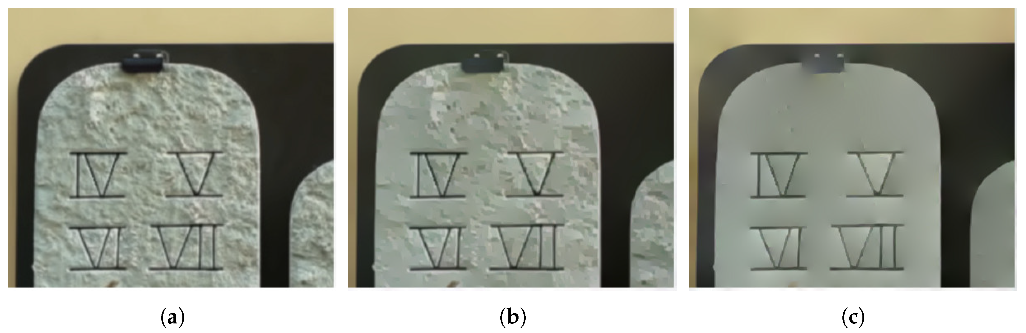
Input image and its horizontal and vertical gradients in absolute values. (a) Input; (b) absolute value of the horizontal gradient; (c) absolute value of the vertical gradient.
Figure 1.
Input image and its horizontal and vertical gradients in absolute values. (a) Input; (b) absolute value of the horizontal gradient; (c) absolute value of the vertical gradient.

Figure 2.
Construction of the target edge-histogram. (a) Histogram of gradient ; (b) histogram of thresholded gradient .
Figure 2.
Construction of the target edge-histogram. (a) Histogram of gradient ; (b) histogram of thresholded gradient .

Figure 3.
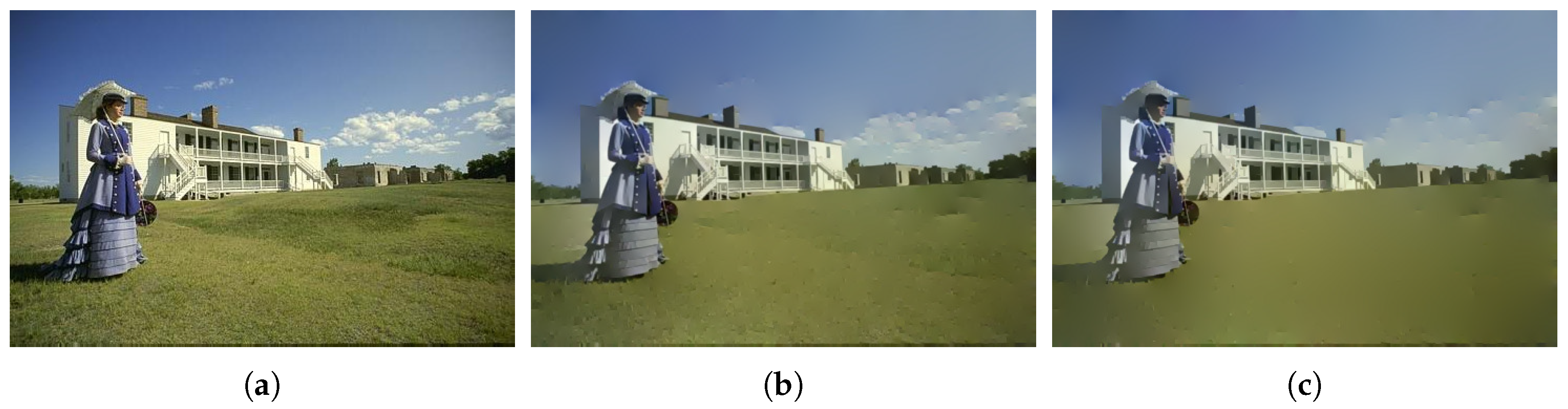
Output of (5) with different . (a) Input; (b) output using ; (c) output using .
Figure 3.
Output of (5) with different . (a) Input; (b) output using ; (c) output using .

Figure 4.
Output of solving (5) repeatedly with , . (a) Input image I; (b) image after one iteration; (c) image after three iterations.
Figure 4.
Output of solving (5) repeatedly with , . (a) Input image I; (b) image after one iteration; (c) image after three iterations.

Figure 5.
Comparison of our method with other methods in image abstraction. (a) Input; (b) Bilateral [18] with ; (c) WLS [21] with ; (d) -smoothing (http://www.cse.cuhk.edu.hk/leojia/projects/L0smoothing/ImageSmoothing.htm) [24]; (e) -projection [29] with ; (f) ours with , .
Figure 5.
Comparison of our method with other methods in image abstraction. (a) Input; (b) Bilateral [18] with ; (c) WLS [21] with ; (d) -smoothing (http://www.cse.cuhk.edu.hk/leojia/projects/L0smoothing/ImageSmoothing.htm) [24]; (e) -projection [29] with ; (f) ours with , .

Figure 6.
Comparison of our method with other methods in edge extraction. (a) Input; (b) Bilateral [18] with ; (c) WLS [21] with ; (d) -smoothing (http://www.cse.cuhk.edu.hk/leojia/projects/L0smoothing/EdgeEnhancement.htm) [24]; (e) -projection [29] with ; (f) ours with , .
Figure 6.
Comparison of our method with other methods in edge extraction. (a) Input; (b) Bilateral [18] with ; (c) WLS [21] with ; (d) -smoothing (http://www.cse.cuhk.edu.hk/leojia/projects/L0smoothing/EdgeEnhancement.htm) [24]; (e) -projection [29] with ; (f) ours with , .

Figure 7.
Applying Canny edge detector to the grayscale version of Figure 6. (a) Input; (b) Bilateral [18]; (c) WLS [21]; (d) -smoothing [24]; (e) -projection [29]; (f) ours.

Figure 8.
Steps to obtain a details-exaggerated image J. (a) Input I; (b) output X from (5) with , ; (c) ; (d) details-exaggerated image .
Figure 8.
Steps to obtain a details-exaggerated image J. (a) Input I; (b) output X from (5) with , ; (c) ; (d) details-exaggerated image .

Figure 9.
Comparison of our method with other methods in details exaggeration. (a) Input; (b) Bilateral [18] with , ; (c) WLS (http://www.cs.huji.ac.il/danix/epd/MSTM/flower/index.html) [21]; (d) -smoothing (http://www.cse.cuhk.edu.hk/leojia/projects/L0smoothing/ToneMapping.htm) [24]; (e) -projection [29] with ; (f) ours with , , .

Figure 10.
Background region detection for three different inputs. Red-colored squares are the regions located by our procedure.
Figure 10.
Background region detection for three different inputs. Red-colored squares are the regions located by our procedure.

Figure 11.
Comparison of our method to a blind method in scan-through removal. (a) Nishida and Suzuki [43] with , ; (b) ours with , , .
Figure 11.
Comparison of our method to a blind method in scan-through removal. (a) Nishida and Suzuki [43] with , ; (b) ours with , , .

© 2018 by the authors. Licensee MDPI, Basel, Switzerland. This article is an open access article distributed under the terms and conditions of the Creative Commons Attribution (CC BY) license (http://creativecommons.org/licenses/by/4.0/).
Share and Cite
MDPI and ACS Style
Chan, K.C.K.; Chan, R.H.; Nikolova, M. A Convex Model for Edge-Histogram Specification with Applications to Edge-Preserving Smoothing. Axioms 2018, 7, 53. https://doi.org/10.3390/axioms7030053
AMA Style
Chan KCK, Chan RH, Nikolova M. A Convex Model for Edge-Histogram Specification with Applications to Edge-Preserving Smoothing. Axioms. 2018; 7(3):53. https://doi.org/10.3390/axioms7030053
Chicago/Turabian StyleChan, Kelvin C. K., Raymond H. Chan, and Mila Nikolova. 2018. "A Convex Model for Edge-Histogram Specification with Applications to Edge-Preserving Smoothing" Axioms 7, no. 3: 53. https://doi.org/10.3390/axioms7030053
Note that from the first issue of 2016, this journal uses article numbers instead of page numbers. See further details here.