On a Class of Hermite-Obreshkov One-Step Methods with Continuous Spline Extension

Abstract

The class of A-stable symmetric one-step Hermite–Obreshkov (HO) methods introduced by F. Loscalzo in 1968 for dealing with initial value problems is analyzed. Such schemes have the peculiarity of admitting a multiple knot spline extension collocating the differential equation at the mesh points. As a new result, it is shown that these maximal order schemes are conjugate symplectic up to order $p+r,$ where $r=2$ and p is the order of the method, which is a benefit when the methods have to be applied to Hamiltonian problems. Furthermore, a new efficient approach for the computation of the spline extension is introduced, adopting the same strategy developed for the BS linear multistep methods. The performances of the schemes are tested in particular on some Hamiltonian benchmarks and compared with those of the Gauss–Runge–Kutta schemes and Euler–Maclaurin formulas of the same order.

1. Introduction

We are interested in the numerical solution of the Cauchy problem, that is the first order Ordinary Differential Equation (ODE),

$${\mathbf{y}}^{\prime }(t)=\mathbf{f}(\mathbf{y}(t)),t\in [t_0,t_0+T],$$

(1)

associated with the initial condition:

$$\mathbf{y}(t_0)={\mathbf{y}}_0,$$

(2)

where $\mathbf{f}:{\mathrm{I}\mathrm{R}}^m\to {\mathrm{I}\mathrm{R}}^m,m\ge 1,$ is a $C^{R-1},R\ge 1,$ function on its domain and ${\mathbf{y}}_0\in {\mathrm{I}\mathrm{R}}^m$ is assigned. Note that there is no loss of generality in assuming that the equation is autonomous. In this context, here, we focus on one-step Hermite–Obreshkov (HO) methods ([1], p. 277). Unlike Runge–Kutta schemes, a high order of convergence is obtained with HO methods without adding stages. Clearly, there is a price for this because total derivatives of the $\mathbf{f}$ function are involved in the difference equation defining the method, and thus, a suitable smoothness requirement for $\mathbf{f}$ is necessary. Multiderivative methods have been considered often in the past for the numerical treatment of ODEs, for example also in the context of boundary value methods [2], and in the last years, there has been a renewed interest in this topic, also considering its application to the numerical solution of differential algebraic equations; see, e.g., [3,4,5,6,7,8]. Here, we consider the numerical solution of Hamiltonian problems which in canonical form can be written as follows:

$${\mathbf{y}}^{\prime }=J\nabla H(\mathbf{y}),\mathbf{y}(t_0)={\mathbf{y}}_0\in {\mathrm{I}\mathrm{R}}^{2\ell },$$

(3)

with:

$$\mathbf{y}=\left(\begin{array}{c}\mathbf{q}\\ \mathbf{p}\end{array}\right),\mathbf{q},\mathbf{p}\in {\mathrm{I}\mathrm{R}}^{\ell },J=\left(\begin{array}{cc}\hfill O& \hfill I_{\ell }\\ \hfill -I_{\ell }& \hfill O\end{array}\right),$$

(4)

where $\mathbf{q}$ and $\mathbf{p}$ are the generalized coordinates and momenta, $H:{\mathrm{I}\mathrm{R}}^{2\ell }\to \mathrm{I}\mathrm{R}$ is the Hamiltonian function and $I_{\ell }$ stands for the identity matrix of dimension ℓ. Note that the flow ${\phi }_t:{\mathbf{y}}_0\to \mathbf{y}(t)$ associated with the dynamical system (3) is symplectic; this means that its Jacobian satisfies:

$$\frac{\partial {\phi }_t{(\mathbf{y})}^{\top }}{\partial \mathbf{y}}J\frac{\partial {\phi }_t(\mathbf{y})}{\partial \mathbf{y}}=J,\forall \mathbf{y}\in {\mathrm{I}\mathrm{R}}^{2\ell }.$$

(5)

A one-step numerical method ${\mathsf{\Phi }}_h:{\mathrm{I}\mathrm{R}}^{2\ell }\to {\mathrm{I}\mathrm{R}}^{2\ell }$ with stepsize h is symplectic if the discrete flow ${\mathbf{y}}_{n+1}={\mathsf{\Phi }}_h({\mathbf{y}}_n),n\ge 0,$ satisfies:

$$\frac{\partial {\mathsf{\Phi }}_h{(\mathbf{y})}^{\top }}{\partial \mathbf{y}}J\frac{\partial {\mathsf{\Phi }}_h(\mathbf{y})}{\partial \mathbf{y}}=J,\forall \mathbf{y}\in {\mathrm{I}\mathrm{R}}^{2\ell }.$$

(6)

Two numerical methods ${\mathsf{\Phi }}_h,{\mathsf{\Psi }}_h$ are conjugate to each other if there exists a global change of coordinates ${\chi }_h$, such that:

$${\mathsf{\Psi }}_h={\chi }_h\circ {\mathsf{\Phi }}_h\circ {\chi }_h^{-1}$$

with ${\chi }_h(\mathbf{y})=\mathbf{y}+O(h)$ uniformly for $\mathbf{y}$ varying in a compact set and ∘ denoting a composition operator [9]. A method which is conjugate to a symplectic method is said to be conjugate symplectic, this is a less strong requirement than symplecticity, which allows the numerical solution to have the same long-time behavior of a symplectic method. Observe that the conjugate symplecticity here refers to a property of the discrete flow of the two numerical methods; this should be not confused with the group of conjugate symplectic matrices, the set of matrices $M\in {\mathbb{C}}^{2\ell }$ that satisfy $M^{H}JM=J$, where H means Hermitian conjugate [10].

A more relaxed property, shared by a wider class of numerical schemes, is a generalization of the conjugate-symplecticity property, introduced in [11]. A method ${\mathbf{y}}_1={\mathsf{\Psi }}_h({\mathbf{y}}_0)$ of order p is conjugate-symplectic up to order $p+r$, with $r\ge 0$, if a global change of coordinates ${\chi }_h(\mathbf{y})=\mathbf{y}+O(h^p)$ exists such that ${\mathsf{\Psi }}_h={\chi }_h\circ {\mathsf{\Phi }}_h\circ {\chi }_h^{-1}$, with the map ${\mathsf{\Psi }}_h$ satisfying

$$\frac{\partial {\mathsf{\Psi }}_h{(\mathbf{y})}^{\top }}{\partial \mathbf{y}}J\frac{\partial {\mathsf{\Psi }}_h(\mathbf{y})}{\partial \mathbf{y}}=J+O(h^{p+r+1}).$$

(7)

A consequence of property (7) is that the method ${\mathsf{\Psi }}_h(\mathbf{y})$ nearly conserves all quadratic first integrals and the Hamiltonian function over time intervals of length $O(h^{-r})$ (see [11]).

Recently, the class of Euler–Maclaurin methods for the solution of Hamiltonian problems has been analyzed in [12,13] where the conjugate symplecticity up to order $p+2$ of the p-th order methods was proven.

In this paper, we consider the symmetric one-step HO methods, which were analyzed in [14,15] in the context of spline applications. We call them BSHO methods, since they are connected to B-Splines, as we will show. BSHO methods have a formulation similar to that of the Euler–Maclaurin formulas, and the order two and four schemes of the two families are the same. As a new result, we prove that BSHO methods are conjugate symplectic schemes up to order $p+2$, as is the case for the Euler–Maclaurin methods [12,13], and so, both families are suited to the context of geometric integration.

BSHO methods are also strictly related to BS methods [16,17], which are a class of linear multistep methods also based on B-splines suited for addressing boundary value problems formulated as first order differential problems. Note that also BS methods were firstly studied in [14,15], but at that time, they were discarded in favor of BSHO methods since; when used as initial value methods, they are not convergent. In [16,17], the same schemes have been studied as boundary value methods, and they have been recovered in particular in connection with boundary value problems. As for the BSHO methods, the discrete solution generated by a BS method can be easily extended to a continuous spline collocating the differential problem at the mesh points [18]. The idea now is to rely on B-splines with multiple inner knots in order to derive one-step HO schemes. The inner knot multiplicity is strictly connected to the number of derivatives of $\mathbf{f}$ involved in the difference equations defining the method and consequently with the order of the method. The efficient approach introduced in [18] dealing with BS methods for the computation of the collocating spline extension is here extended to BSHO methods, working with multiple knots. Note that we adopt a reversed point of view with respect to [14,15] because we assume to have already available the numerical solution generated by the BSHO methods and to be interested in an efficient procedure for obtaining the B-spline coefficients of the associated spline.

The paper is organized as follows. In Section 2, one-step symmetric HO methods are introduced, focusing in particular on BSHO methods. Section 3 is devoted to proving that BSHO methods are conjugate symplectic methods up to order $p+2$. Then, Section 4 first shows how these methods can be revisited in the spline collocation context. Successively, an efficient procedure is introduced to compute the B-spline form of the collocating spline extension associated with the numerical solution produced by the R-th BSHO, and it is shown that its convergence order is equal to that of the numerical solution. 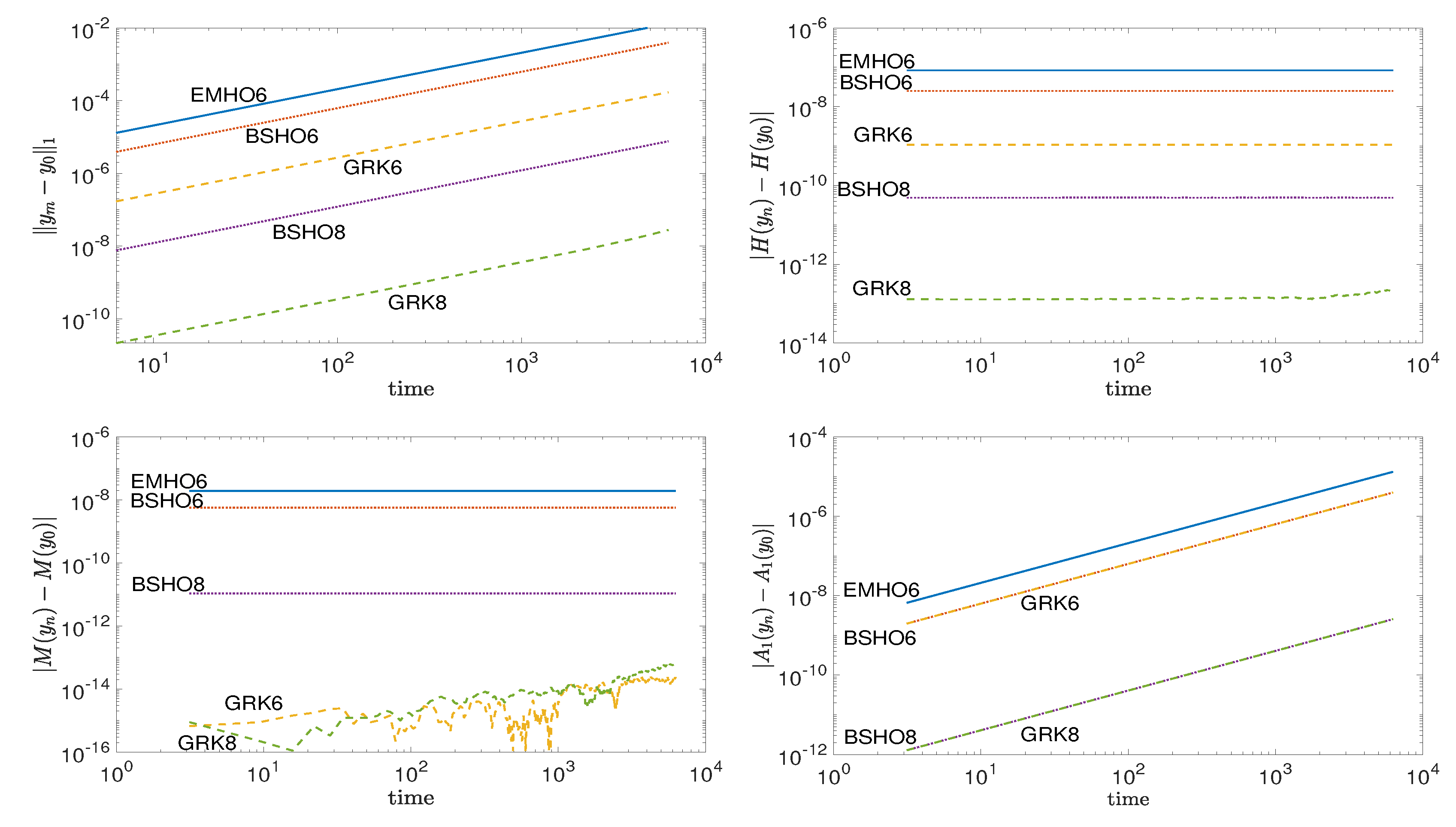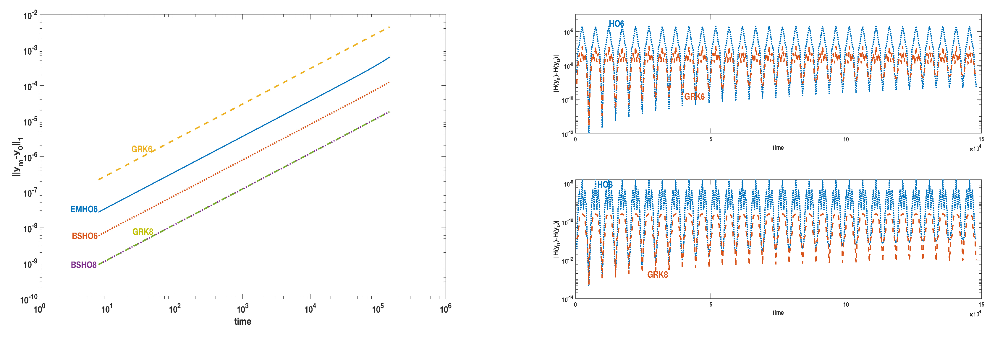Section 6 presents some numerical results related to Hamiltonian problems, comparing them with those generated by Euler–Maclaurin and Gauss–Runge–Kutta schemes of the same order.

2. One-Step Symmetric Hermite–Obreshkov Methods

Let $t_i,i=0,\dots ,N,$ be an assigned partition of the integration interval $[t_0,t_0+T]$, and let us denote by ${\mathbf{u}}_i$ an approximation of $\mathbf{y}(t_i)$. Any one-step symmetric Hermite–Obreshkov (HO) method can be written as follows, clearly setting ${\mathbf{u}}_0:={\mathbf{y}}_0,$

$${\displaystyle {\mathbf{u}}_{n+1}={\mathbf{u}}_n+\sum _{j=1}^R{h}_n^j{\beta }_j^{(R)}\left({\mathbf{u}}_n^{(j)}-{(-1)}^j{\mathbf{u}}_{n+1}^{(j)}\right),n=0,\dots ,N-1,}$$

(8)

where $h_n:=t_{n+1}-t_n$ and where ${\mathbf{u}}_r^{(j)}$, for $j\ge 1,$ denotes the total $(j-1)$-th derivative of $\mathbf{f}$ with respect to t computed at ${\mathbf{u}}_r$,

$${\mathbf{u}}_r^{(j)}:=\frac{d^{j-1}\mathbf{f}}{d{t}^{j-1}}{(\mathbf{y}(t))|}_{{\mathbf{u}}_r},j=1,\dots ,R.$$

(9)

Note that ${\mathbf{u}}_r^{(j)}\approx {\mathbf{y}}^{(j)}(t_r)$, and on the basis of (1), the analytical computation of the j-th derivative ${\mathbf{y}}^{(j)}$ involves a tensor of order j. For example, ${\mathbf{y}}^{(2)}(t)=\frac{d\mathbf{f}}{dt}(\mathbf{y}(t))=\frac{\partial \mathbf{f}}{\partial \mathbf{y}}(\mathbf{y}(t))\mathbf{f}(\mathbf{y}(t))$ (where $\frac{\partial \mathbf{f}}{\partial \mathbf{y}}$ becomes the Jacobian $m\times m$ matrix of $\mathbf{f}$ with respect to $\mathbf{y}$ when $m>1$). As a consequence, it is ${\mathbf{u}}_r^{(2)}=\frac{\partial \mathbf{f}}{\partial \mathbf{y}}({\mathbf{u}}_r)\mathbf{f}({\mathbf{u}}_r).$ We observe that the definition in (14) implies that only ${\mathbf{u}}_{n+1}$ is unknown in (8), which in general is a nonlinear vector equation in ${\mathrm{I}\mathrm{R}}^m$ with respect to it.

For example, the one-step Euler–Maclaurin [1] formulas of order $2s$ with $s\in \mathrm{I}\mathrm{N},s\ge 1,$

$$\begin{array}{cc}\hfill {\mathbf{u}}_{n+1}& {\displaystyle ={\mathbf{u}}_n+\frac{h_n}{2}\left({\mathbf{u}}_n^{(1)}+{\mathbf{u}}_{n+1}^{(1)})\right)+\sum _{i=1}^{s-1}{h}_n^{2i}\frac{b_{2i}}{(2i)!}\left({\mathbf{u}}_n^{(2i)}-{\mathbf{u}}_{n+1}^{(2i)}\right),n=0,\dots ,N-1,}\hfill \end{array}$$

(10)

(where the $b_{2i}$ denote the Bernoulli numbers, which are reported in Table 2) belong to this class of methods. These methods will be referred to in the following with the label EMHO (Euler–Maclaurin Hermite–Obreshkov).

Here, we consider another class of symmetric HO methods that can be obtained by defining as follows the polynomial $P_{2R},$

$$P_{2R}(x):=\frac{x^R{(x-1)}^R}{(2R)!}$$

(11)

appearing in ([1], Lemma 13.3), the statement of which is reported in Lemma 1.

Lemma 1.

Let R be any positive integer and $P_{2R}$ be a polynomial of exact degree $2R$. Then, the following one-step linear difference equation,

$$\sum _{j=0}^{2R}{h}_n^j{\mathbf{u}}_{n+1}^{(j)}{P}_{2R}^{(2R-j)}(0)=\sum _{j=0}^{2R}{h}_n^j{\mathbf{u}}_n^{(j)}{P}_{2R}^{(2R-j)}(1)$$

defines a multiderivative method of order $2R$.

Referring to the methods obtainable by Lemma 1, if in particular the polynomial $P_{2R}$ is defined as in (11), then we obtain the class of methods in which we are interested here. They can be written as in (8) with,

$${\beta }_j^{(R)}:=\frac{1}{j!}\frac{R(R-1)\cdots (R-j+1)}{(2R)(2R-1)\cdots (2R-j+1)}$$

(12)

which are reported in

Table 1. Symmetric one-step B-Spline Hermite–Obreshkov (BSHO) coefficients.

R	${\mathit{\beta }}_1^{(\mathit{R})}$	${\mathit{\beta }}_2^{(\mathit{R})}$	${\mathit{\beta }}_3^{(\mathit{R})}$	${\mathit{\beta }}_4^{(\mathit{R})}$	${\mathit{\beta }}_5^{(\mathit{R})}$
1	$\frac{1}{2}$
2	$\frac{1}{2}$	$\frac{1}{12}$
3	$\frac{1}{2}$	$\frac{1}{10}$	$\frac{1}{120}$
4	$\frac{1}{2}$	$\frac{3}{28}$	$\frac{1}{84}$	$\frac{1}{1680}$
5	$\frac{1}{2}$	$\frac{1}{9}$	$\frac{1}{72}$	$\frac{1}{1008}$	$\frac{1}{30240}$

, for $R=1,\dots ,5$. In particular, for $R=1$ and $R=2$, we obtain the trapezoidal rule and the Euler–Maclaurin method of order four, respectively.

These methods were originally introduced in the spline collocation context, dealing in particular with splines with multiple knots [14,15], as we will show in Section 4. We call them BSHO methods since we will show that they can be obtained dealing in particular with the standard B-spline basis. The stability function of the R-th one-step symmetric BSHO method is the rational function corresponding to the $(R,R)$-Padé approximation of the exponential function, as is that of the same order Runge–Kutta–Gauss method ([19], p. 72). It has been proven that methods with this stability function are A-stable ([19], Theorem 4.12). For the proof of the statement of the following corollary, which will be useful in the sequel, we refer to [15],

Corollary 1.

Let us assume that $\mathbf{f}\in C^{2R+1}(\mathcal{D}),$ where $\mathcal{D}:=\{\mathbf{y}\in {\mathrm{I}\mathrm{R}}^m|\exists t\in [t_0,t_0+T]$ such that ${\parallel \mathbf{y}-\mathbf{y}(t)\parallel }_2\le L_b\},$ with $L_b>0.$ Then, there exists a positive constant $h_b$ such that if ${\displaystyle \underset{0\le n\le N-1}{max}{h}_n=:h<h_b}$ and ${\left\{{\mathbf{u}}_i\right\}}_{i=0}^N$ denotes the related numerical solution produced by the R-th one-step symmetric BSHO method in (8)–(12), it is:

$$\parallel {\mathbf{u}}_i^{(j)}-{\mathbf{y}}_i^{(j)}\parallel =O(h^{2R}),j=1,\dots ,R,i=0,\dots ,N.$$

3. Conjugate Symplecticity of the Symmetric One-Step BSHO Methods

Following the lines of the proof given in [13], in this section, we prove that one-step symmetric BSHO methods are conjugate symplectic schemes up to order $2R+2$. The following lemma, proved in [20], is the starting point of the proof, and it makes use of the B-series integrator concept. On this concern, referring to [9] for the details, here, we just recall that a B-series integrator is a numerical method that can be expressed as a formal B-series, that is it has a power series in the time step in which each term is a sum of elementary differentials of the vector field and where the number of terms is allowed to be infinite.

Lemma 2.

Assume that Problem (1) admits a quadratic first integral $Q(\mathbf{y})={\mathbf{y}}^{T}S\mathbf{y}$ (with S denoting a constant symmetric matrix) and that it is solved by a B-series integrator ${\mathsf{\Phi }}_h(\mathbf{y})$. Then, the following properties, where all formulas have to be interpreted in the sense of formal series, are equivalent:

(a) 

${\mathsf{\Phi }}_h(\mathbf{y})$ has a modified first integral of the form $\tilde{Q}(\mathbf{y})=Q(\mathbf{y})+h{Q}_1(\mathbf{y})+h^2{Q}_2(\mathbf{y})+...$ where each $Q_i(·)$ is a differential functional;

(b) 

${\mathsf{\Phi }}_h(\mathbf{y})$ is conjugate to a symplectic B-series integrator.

We observe that Lemma 2 is used in [21] to prove the conjugate symplecticity of symmetric linear multistep methods. Following the lines of the proof given in [13], we can actually prove that the R-th one-step symmetric BSHO method is conjugate symplectic up to order $2R+2$. With similar arguments of [13] we prove the following theorem, showing that the map ${\mathbf{y}}_1={\mathsf{\Psi }}_h({\mathbf{y}}_0)$ associated with the BSHO method is such that ${\mathsf{\Psi }}_h(\mathbf{y})={\mathsf{\Phi }}_h(\mathbf{y})+O(h^{2R+3})$, where ${\mathbf{y}}_1={\mathsf{\Phi }}_h({\mathbf{y}}_0)$ is a suitable conjugate symplectic B-series integrator.

Theorem 1.

The map ${\mathbf{u}}_1={\mathsf{\Psi }}_h({\mathbf{u}}_0)$ associated with the one-step method (8) admits a B-series expansion and is conjugate to a symplectic B-series integrator up to order $2R+2$.

Proof. 

The existence of a B-series expansion for ${\mathbf{y}}_1={\mathsf{\Psi }}_h({\mathbf{y}}_0)$ is directly deduced from [22], where a B-series representation of a generic multi-derivative Runge-Kutta method has been obtained. By defining the two characteristic polynomials of the trapezoidal rule:

$$\rho (z):=z-1,\sigma (z):=\frac{1}{2}(z+1)$$

and the shift operator $E({\mathbf{u}}_n):={\mathbf{u}}_{n+1},$ the R-th method described in (8) reads,

$$\rho (E){\mathbf{u}}_n=\sum _{k=1}^{\lceil R/2\rceil }2{\beta }_{2k-1}^{(R)}{h}^{2k-1}\sigma (E){\mathbf{u}}_n^{(2k-1)}-\sum _{k=1}^{\lfloor R/2\rfloor }{\beta }_{2k}^{(R)}{h}^{2k}\rho (E){\mathbf{u}}_n^{(2k)}.$$

(13)

Observe that ${\mathbf{u}}_i^{(j)}$, for $j\ge 1,$ denotes the $(j-1)$-th Lie derivative of $\mathbf{f}$ computed at ${\mathbf{u}}_i$,

$${\mathbf{u}}_i^{(j)}:=D_{j-1}\mathbf{f}({\mathbf{u}}_i),j=1,\dots ,R,$$

(14)

where $D_0=I$ is the identity operator and $D_k\mathbf{f}(\mathbf{z})$ is defined as the k-th total derivative of $\mathbf{f}(\mathbf{y}(t))$ computed at $\mathbf{y}(t)=\mathbf{z},$ where for the computation of the total derivative it is assumed that $\mathbf{y}$ satisfies the differential equation in (1). Note that we use the subscript to define the Lie operator to avoid confusion with the same order classical derivative operator in the following denoted as $D^k.$ With this clarification on the definition of ${\mathbf{u}}_i^{(j)},$ we now consider a function $\mathbf{v}(t)$, a stepsize h and the shift operator $E_h(\mathbf{v}(t)):=\mathbf{v}(t+h)$, and we look for a continuous function $\mathbf{v}(t)$ that satisfies (13) in the sense of formal series (a series where the number of terms is allowed to be infinite), using the relation $E_h={\sum }_{j=0}^{\infty }\frac{h^j}{j!}{D}^j\equiv e^{hD}$ where $D=D^1$ is the classical derivative operator,

$$\rho (e^{hD})\mathbf{v}(t)=\sum _{k=1}^{\lceil R/2\rceil }2{\beta }_{2k-1}^{(R)}{h}^{2k-1}\sigma (e^{hD})D_{2k-2}\mathbf{f}(\mathbf{v}(t))-\sum _{k=1}^{\lfloor R/2\rfloor }{\beta }_{2k}^{(R)}{h}^{2k}\rho (e^{hD})D_{2k-1}\mathbf{f}(\mathbf{v}(t)).$$

By multiplying both sides of the previous equation by $D\rho {(e^{hD})}^{-1}$, we obtain:

$$D\mathbf{v}(t)=hD\rho {(e^{hD})}^{-1}\sigma (e^{hD})\sum _{k=0}^{\lceil R/2\rceil -1}2{\beta }_{2k+1}^{(R)}{h}^{2k}{D}_{2k}\mathbf{f}(\mathbf{v}(t))-\sum _{k=1}^{\lfloor R/2\rfloor }{\beta }_{2k}^{(R)}{h}^{2k}D{D}_{2k-1}\mathbf{f}(\mathbf{v}(t)).$$

(15)

Now, since Bernoulli numbers define the Taylor expansion of the function $z/(e^z-1)$ and $b_0=1,b_1=-1/2$ and $b_j=0$ for the other odd $j,$ we have:

$$\frac{z\sigma (e^z)}{\rho (e^z)}=\frac{1}{2}\frac{z(e^z+1)}{e^z-1}=\frac{z}{e^z-1}+\frac{z}{2}=1+\sum _{j=1}^{\infty }\frac{b_{2j}}{(2j)!}{z}^{2j}.$$

Thus, we can write (15) as

$$\dot{\mathbf{v}}(t)=\left(\left(I+\sum _{j=1}^{\infty }\frac{b_{2j}}{(2j)!}{h}^{2j}{D}^{2j}\right)\left(I+\sum _{k=1}^{\lceil R/2\rceil -1}2{\beta }_{2k+1}^{(R)}{h}^{2k}{D}_{2k}\right)-\sum _{k=1}^{\lfloor R/2\rfloor }{\beta }_{2k}^{(R)}{h}^{2k}D{D}_{2k-1}\right)\mathbf{f}(\mathbf{v}(t)).$$

Adding and subtracting terms involving the classical derivative operator $D^{2k},D^{2k-1}$, we get

$$\begin{array}{cc}\hfill \dot{\mathbf{v}}(t)=& \left(\left(I+\sum _{j=1}^{\infty }\frac{b_{2j}}{(2j)!}{h}^{2j}{D}^{2j}\right)\right.\hfill \\ & \left(I+\sum _{k=1}^{\lceil R/2\rceil -1}2{\beta }_{2k+1}^{(R)}{h}^{2k}{D}^{2k}+\sum _{k=1}^{\lceil R/2\rceil -1}2{\beta }_{2k+1}^{(R)}{h}^{2k}(D_{2k}-D^{2k})\right)\hfill \\ & -\left.\sum _{k=1}^{\lfloor R/2\rfloor }{\beta }_{2k}^{(R)}{h}^{2k}D{D}^{2k-1}-\sum _{k=1}^{\lfloor R/2\rfloor }{\beta }_{2k}^{(R)}{h}^{2k}D(D_{2k-1}-D^{2k-1})\right)\mathbf{f}(\mathbf{v}(t)).\hfill \end{array}$$

that we recast as

$$\begin{array}{cc}\hfill \dot{\mathbf{v}}(t)=& \left(\left(I+\sum _{j=1}^{\infty }\frac{b_{2j}}{(2j)!}{h}^{2j}{D}^{2j}\right)\left(I+\sum _{k=1}^{\lceil R/2\rceil -1}2{\beta }_{2k+1}^{(R)}{h}^{2k}{D}^{2k}\right)\right.\hfill \\ \hfill & -\left.\sum _{k=1}^{\lfloor R/2\rfloor }{\beta }_{2k}^{(R)}{h}^{2k}{D}^{2k}\right)\mathbf{f}(\mathbf{v}(t))\hfill \\ \hfill & +\left(\left(I+\sum _{j=1}^{\infty }\frac{b_{2j}}{(2j)!}{h}^{2j}{D}^{2j}\right)\left(\sum _{k=1}^{\lceil R/2\rceil -1}2{\beta }_{2k+1}^{(R)}{h}^{2k}(D_{2k}-D^{2k})\right)\right.\hfill \\ \hfill & -\left.\sum _{k=1}^{\lfloor R/2\rfloor }{\beta }_{2k}^{(R)}{h}^{2k}D(D_{2k-1}-D^{2k-1})\right)\mathbf{f}(\mathbf{v}(t)).\hfill \end{array}$$

(16)

Since $\mathbf{v}(t)=\mathbf{y}(t)+O(h^{2R})$, due to the regularity conditions on the function $\mathbf{f}$, we see that $(D^i-D_i)\mathbf{f}(\mathbf{v}(t))=O(h^{2R}),i=1,\cdots ,R-1$ and hence the solution $\mathbf{v}(t)$ of (16) is $O(h^{2R+2})$-close to the solution of the following initial value problem

$$\dot{\mathbf{w}}(t)=\mathbf{f}(\mathbf{w}(t))+\sum _{j=R}^{\infty }{\delta }_j{h}^{2j}{D}^{2j}\mathbf{f}(\mathbf{w}(t)),$$

(17)

with:

$${\delta }_j:=\sum _{k=0}^{\lceil R/2\rceil -1}\frac{b_{2(j-k)}}{(2(j-k))!}2{\beta }_{2k+1}^{(R)},j\ge R.$$

that has been derived from (16) by neglecting the sums containing the derivatives $D_{2k},D_{2k-1}$. Observe that ${\delta }_j=0$ for $j=1,\cdots ,R-1,$ since the method is of order $2R$ (see [9], Theorem 3.1, page 340). We may interpret (17) as the modified equation of a one-step method ${\mathbf{y}}_1={\mathsf{\Phi }}_h({\mathbf{y}}_0)$, where ${\mathsf{\Phi }}_h$ is evidently the time-h flow associated with (17). Expanding the solution of (17) in Taylor series, we get the modified initial value differential equation associated with the numerical scheme by coupling (17) with the initial condition $\mathbf{w}(t_0)={\mathbf{y}}_0$. Thus, ${\mathsf{\Phi }}_h$ is a B-series integrators. The proof of the conjugated symplecticity of ${\mathsf{\Phi }}_h$ follows exactly the same steps of the analogous proof in Theorem 1 of [13]. Since ${\mathsf{\Psi }}_h(\mathbf{y})={\mathsf{\Phi }}_h(\mathbf{y})+O(h^{2R+3})$ and ${\mathsf{\Phi }}_h$ is conjugate-symplectic, the result follows using the same global change of coordinates ${\chi }_h(\mathbf{y})$ associated to ${\mathsf{\Phi }}_h$. ☐

In

Table 2. Coefficients of the modified differential equations and Bernoulli numbers.

R	1	2	3	4	5
${\delta }_R$	$\frac{b_2}{2!}$	$\frac{b_4}{4!}$	$\frac{3}{10}\frac{b_6}{6!}$	$\frac{1}{21}\frac{b_8}{8!}$	$\frac{1}{210}\frac{b_{10}}{10!}$
$b_{2R}$	$\frac{1}{6}$	$-\frac{1}{30}$	$\frac{1}{42}$	$-\frac{1}{30}$	$\frac{5}{66}$

, we report the coefficients ${\delta }_R$ for $R\le 5$ and the corresponding Bernoulli numbers. We can observe that the truncation error in the modified initial value problem is smaller than the one of the EMHO methods of the same order, which is equal to $b_i/i!$ (see [13]). The conjugate symplecticity up to order $2R+2$ property of a numerical scheme makes it suitable for the solution of Hamiltonian problems. A well-known pair of conjugate symplectic methods is composed by the trapezoidal and midpoint rules. Observe that the trapezoidal rule belongs to both the classes BSHO and EMHO of multiderivative methods, and its characteristic polynomial plays an important role in the proof of Theorem 1.

4. The Spline Extension

A (vector) Hermite polynomial of degree $2R+1$ interpolating both ${\mathbf{u}}_n$ and ${\mathbf{u}}_{n+1}$ respectively at $t_n$ and $t_{n+1}$ together with assigned derivatives ${\mathbf{u}}_n^{(k)},{\mathbf{u}}_{n+1}^{(k)},k=1,\dots ,R,$ can be computed using the Newton interpolation formulas with multiple nodes. On the other hand, in his Ph.D. thesis [15], Loscalzo proved that a polynomial of degree $2R$ verifying the same conditions exists if and only if (8) is fulfilled with the $\beta$ coefficients defined as in (12). Note that, since the polynomial of degree $2R+1$ fulfilling these conditions is always unique and its principal coefficient is given by the generalized divided difference $u[t_n,\dots ,t_n,t_{n+1},\dots ,t_{n+1}]$ of order $2R+1$ associated with the given R-order Hermite data, the n-th condition in (8) holds iff this coefficient vanishes. If all the conditions in (8) are fulfilled, it is possible to define a piecewise polynomial, the restriction to $[t_n,t_{n+1}]$ of which coincides with this polynomial, and it is clearly a $C^R$ spline of degree $2R$ with breakpoints at the mesh points. Now, when the definition given in (14) is used together with the assumption ${\mathbf{u}}_0={\mathbf{y}}_0,$ the conditions in (8) become a multiderivative one-step scheme for the numerical solution of (1). Thus, the numerical solution ${\mathbf{u}}_n,n=0,\dots ,N$ it produces and the associated derivative values defined as in (14) can be associated with the above-mentioned $2R$ degree spline extension. Such a spline collocates the differential equation at the mesh points with multiplicity $R,$ that is it verifies the given differential equation and also the equations ${\mathbf{y}}^{(j)}(t)=\frac{d^{(j-1)}(\mathbf{f}\circ \mathbf{y})}{d{t}^{j-1}}(t),j=2,\dots ,R$ at the mesh points. This piecewise representation of the spline is that adopted in [15]. Here, we are interested in deriving its more compact B-spline representation. Besides being more compact, this also allows us to clarify the connection between BSHO and BS methods previously introduced in [16,17,18]. For this aim, let us introduce some necessary notation. Let $S_{2R},$ be the space of $C^R$$2R$-degree splines with breakpoints at $t_i,i=0,\dots ,N,$ where $t_0<\cdots <t_N=t_0+T.$ Since we relate to the B-spline basis, we need to introduce the associated extended knot vector:

$$\mathcal{T}:=\{{\tau }_{-2R},\dots ,{\tau }_{-1},{\tau }_0,\dots ,{\tau }_{(N-1)R},{\tau }_{(N-1)R+1},{\tau }_{(N-1)R+2}\dots ,{\tau }_{(N+1)R+1}\},$$

(18)

where:

$$\begin{array}{cc}\hfill {\tau }_{-2R}& =\cdots ={\tau }_0=t_0,\hfill \\ \hfill {\tau }_{(n-1)R+1}& =\cdots ={\tau }_{nR}=t_n,\hfill & \hfill n=1,\dots ,N-1,\\ \hfill {\tau }_{(N-1)R+1}& =\cdots ={\tau }_{(N+1)R+1}=t_N,\hfill \end{array}$$

which means that all the inner breakpoints have multiplicity R in $\mathcal{T}$ and both $t_0$ and $t_N$ have multiplicity $2R+1.$ The associated B-spline basis is denoted as $B_i,i=-2R,\dots ,(N-1)R$ and the dimension of $S_{2R}$ as $D,$ with $D:=(N+1)R+1.$

The mentioned result proven by Loscalzo is equivalent to saying that, if the $\beta$ coefficients are defined as in (12), any $C^R$ spline of degree $2R$ with breakpoints at the mesh points fulfills the relation in (8), where ${\mathbf{u}}_n^{(j)}$ denotes the j-th spline derivative at $t_n.$ In turn, this is equivalent to saying that such a relation holds for any element of the B-spline basis of $S_{2R}.$ Thus, setting $\mathbf{\alpha }:={(-1;1)}^T\in {\mathrm{I}\mathrm{R}}^2$ and ${\mathbf{\beta }}^{(i)}:=({\beta }_i^{(R)};-{(-1)}^i{\beta }_i^{(R)})\in {\mathrm{I}\mathrm{R}}^2,i=1,\dots ,R,$ considering the local support of the B-spline basis, we have that $(\mathbf{\alpha };{\mathbf{\beta }}^{(1)};...;{\mathbf{\beta }}^{(R)})$, where the punctuation mark “;” means vertical catenation (to make a column-vector), can be also characterized as the unique solution of the following linear system,

$$G^{(n)}(\mathbf{\alpha };{\mathbf{\beta }}^{(1)};\cdots ;{\mathbf{\beta }}^{(R)})={\mathbf{e}}_{2R+2},$$

(19)

where ${\mathbf{e}}_{2R+2}=(0;\dots ;0;1)\in {\mathrm{I}\mathrm{R}}^{2R+2}$ and:

$$G^{(n)}:=\left[\begin{array}{ccccc}\hfill A_1^{(n)T}& \hfill -h_n{A}_2^{(n)T}& \hfill -h_n^2{A}_3^{(n)T}& \hfill \cdots & \hfill -h_n^R{A}_{R+1}^{(n)T}\\ \hfill (0,0)& \hfill (1,1)& \hfill (0,0)& \hfill \cdots & \hfill (0,0)\end{array}\right],$$

(20)

with $A_1^{(n)},A_2^{(n)},\cdots A_{R+1}^{(n)}$ defined as,

$$A_{j+1}^{(n)}:={\left[\begin{array}{ccc}{B}_{(n-2)R}^{(j)}(t_n),& \dots ,& B_{nR}^{(j)}(t_n)\\ B_{(n-2)R}^{(j)}(t_{n+1}),& \dots ,& B_{nR}^{(j)}(t_{n+1})\end{array}\right]}_{2\times (2R+1)}$$

(21)

where $B_i^{(j)}$ denotes the j-th derivative of $B_i.$ Note that the last equation in (19), $2{\beta }_1^{(R)}=1,$ is just a normalization condition.

In order to prove the non-singularity of the matrix $G^{(n)},$ we need to introduce the following definition,

Definition 1.

Given a non-decreasing set of abscissas $\mathsf{\Theta }:={\left\{{\theta }_i\right\}}_{i=0}^M,$ we say that a function $g_1$ agrees with another function $g_2$ at Θ if $g_1^{(j)}({\theta }_i)=g_2^{(j)}({\theta }_i),j=0,\dots ,m_i-1,i=0,\dots ,M,$ where $m_i$ denotes the multiplicity of ${\theta }_i$ in $\mathsf{\Theta }.$

Then, we can formulate the following proposition,

Proposition 1.

The $(2R+2)\times (2R+2)$ matrix $G^{(n)}$ defined in (20) and associated with the B-spline basis of $S_{2R}$ is nonsingular.

Proof. 

Observe that the restriction to $I_n=[t_n,t_{n+1}]$ of the splines in $S_{2R}$ generates ${\Pi }_{2R}$ since there are no inner knots in $I_n.$ Then, restricting to $I_n,{\Pi }_{2R}$ can be also generated by the B-splines of $S_{2R}$ not vanishing in $I_n,$ that is from $B_{(n-2)R},\dots ,B_{nR}.$ Since the polynomial in ${\Pi }_{2R}$ agreeing with a given function in:

$$\mathsf{\Theta }=\{\stackrel{R+1}{\overbrace{t_n,\dots ,t_n}},\stackrel{R}{\overbrace{t_{n+1},\dots ,t_{n+1}}}\},$$

is unique, it follows that also the corresponding $(2R+1)\times (2R+1)$ matrix collocating the spline basis active in $I_n$ is nonsingular. Such a matrix is the principal submatrix of $G^{(n)T}$ of order $2R+1.$ Thus now, considering that the restriction to $I_n$ of any function in $S_{2R}$ is a polynomial of degree $2R,$ we prove by reductio ad absurdum that the last row of $G^{(n)}$ cannot be a linear combination of the other rows. In fact, in the opposite case, there would exist a polynomial P of degree $2R$ such that $P(t_n)=P(t_{n+1})=0,P^{\prime }(t_n)=P^{\prime }(t_{n+1})=-1,$ and $P^{(j)}(t_n)=P^{(j)}(t_{n+1})=0,j=2,\dots ,R.$ Considering the specific interpolation conditions, this P does not fulfill the n-th condition in (8). This is absurd, since Loscalzo [15] has proven that such a condition is equivalent to requiring degree reduction for the unique polynomial of degree less than or equal to $2R+1$, fulfilling $R+1$ Hermite conditions at both $t_n$ and $t_{n+1}.$ ☐

Note that this different form for defining the coefficient of the R-th BSHO scheme is analogous to that adopted in [17] for defining a BS method on a general partition. However, in this case, the coefficients of the scheme do not depend on the mesh distribution, so there is no need to determine them solving the above linear system. On the other hand, having proven that the matrix $G^{(n)}$ is nonsingular will be useful in the following for determining the B-spline form of the associated spline extension.

Thus, let us now see how the B-spline coefficients of the spline in $S_{2R}$ associated with the numerical solution generated by the R-th BSHO can be efficiently obtained, considering that the following conditions have to be imposed,

$$\left\{\begin{array}{cc}{\mathbf{s}}_{2R}(t_n)\hfill & ={\mathbf{u}}_n,\hfill \\ {\mathbf{s}}_{2R}^{(j)}(t_n)\hfill & ={\mathbf{u}}_n^{(j)},j=1,\dots ,R.\hfill \end{array}\right.n=0,\dots ,N.$$

(22)

Now, we are interested in deriving the B-spline coefficients ${\mathbf{c}}_i,i=-2R,\cdots ,(N-1)R,$ of ${\mathbf{s}}_{2R},$

$${\mathbf{s}}_{2R}(t)=\sum _{i=-2R}^{(N-1)R}{\mathbf{c}}_i{B}_i(t),t\in [t_0,t_0+T].$$

(23)

Relying on the representation in (23), all the conditions in (22) can be re-written in the following compact matrix form,

$$(A\otimes I_m)\mathbf{c}=({\mathbf{u}}_0;\dots ;{\mathbf{u}}_N;{\mathbf{u}}_0^{(1)};\dots ;{\mathbf{u}}_N^{(1)};\cdots ;{\mathbf{u}}_0^{(R)};\dots ;{\mathbf{u}}_N^{(R)}),$$

(24)

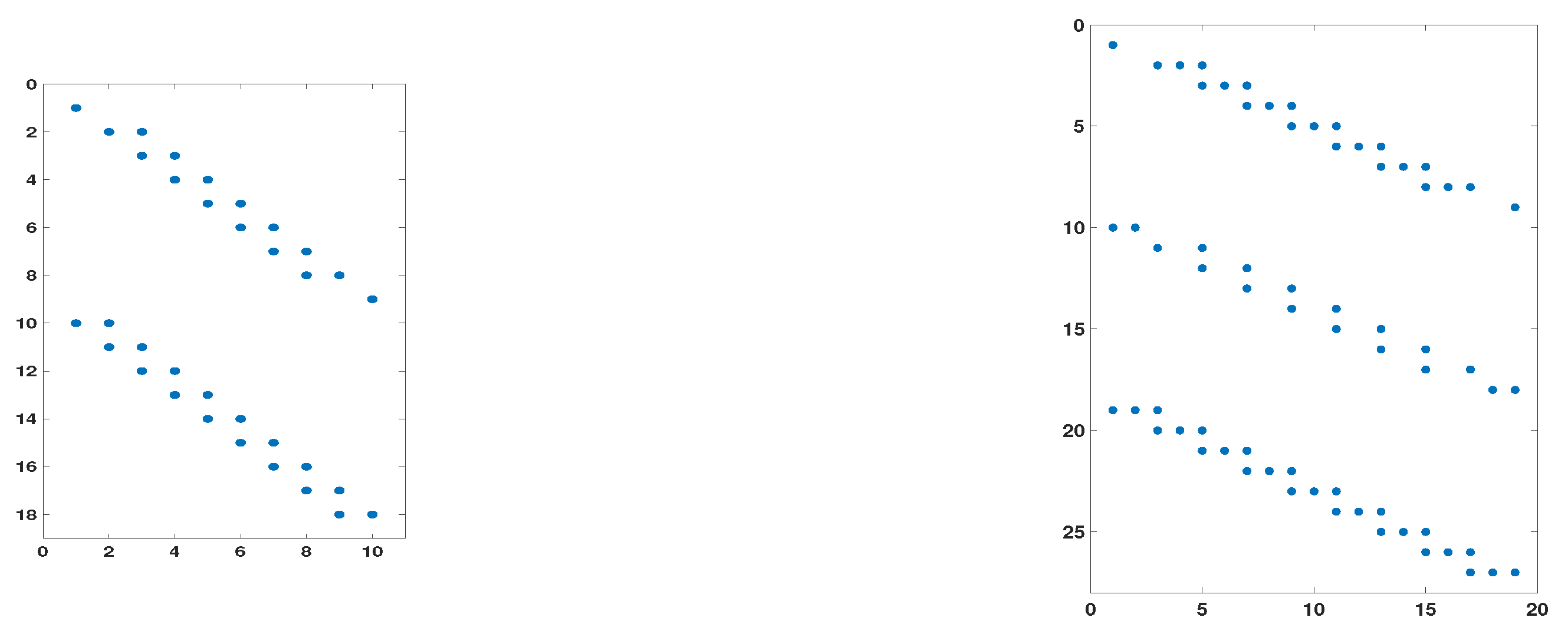
where $\mathbf{c}=({\mathbf{c}}_{-2R};\dots ;{\mathbf{c}}_{(N-1)R})\in {\mathrm{I}\mathrm{R}}^{mD}$, with ${\mathbf{c}}_j\in {\mathrm{I}\mathrm{R}}^m,$$I_m$ is the identity matrix of size $m\times m,$D is the dimension of the spline space previously introduced and where:

$$A:=\left(A_1;A_2;\cdots ;A_{R+1}\right),$$

with each $A_{\ell }$ being a $(R+1)$-banded matrix of size $(N+1)\times D$ (see Figure 1) with entries defined as follows:

$${(A_{\ell })}_{i,j}:=B_j^{(\ell -1)}(t_i).$$

(25)

The following theorem related to the rectangular linear system in (24) ensures that the collocating spline $s_{2R}$ is well defined.

Theorem 2.

The rectangular linear system in (24) has always a unique solution, if the entries of the vector on its right-hand side satisfy the conditions in (8) with the β coefficients given in (12).

Proof. 

The proof is analogous to that in [18] (Theorem 1), and it is omitted. ☐

We now move to introduce the strategy adopted for an efficient computation of the B-spline coefficients of $s_{2R}.$

4.1. Efficient Spline Computation

Concerning the computation of the spline coefficient vectors:

$${\mathbf{c}}_i,i=-(2R),\dots ,(N-1)R,$$

the unique solution of (24) can be computed with several different strategies, which can have very different computational costs and can produce results with different accuracy when implemented in finite arithmetic. Here, we follow the local strategy used in [18]. Taking into account the banded structure of $A_i,i=1,\dots ,R+1$, we can verify that (24) implies the following relations,

$$\left[\begin{array}{c}\hfill A_1^{(i)}\\ \hfill -h_i{A}_2^{(i)}\\ \hfill ⋮\\ \hfill -h_i^R{A}_{R+1}^{(i)}\end{array}\right]\otimes I_m{\mathbf{c}}^{(i)}={\mathbf{w}}^{(i)}(\mathbf{u})$$

(26)

where $\mathbf{u}=({\mathbf{u}}_0;\dots ;{\mathbf{u}}_N),{\mathbf{c}}^{(i)}:=({\mathbf{c}}_{(i-3)R};\dots ;{\mathbf{c}}_{(i-1)R})\in {\mathrm{I}\mathrm{R}}^{m(2R+1)},i=1,\dots ,N$ and:

$${\mathbf{w}}^{(i)}(\mathbf{u}):=({\mathbf{u}}_{i-1};{\mathbf{u}}_i;-h_i{\mathbf{u}}_{i-1}^{(1)};-h_i{\mathbf{u}}_i^{(1)};\dots ;-h_i^R{\mathbf{u}}_{i-1}^{(R)};-h_i^R{\mathbf{u}}_i^{(R)}).$$

As a consequence, we can also write that,

$$(G^{(i)T}\otimes I_m){\widehat{\mathbf{c}}}^{(i)}={\mathbf{w}}^{(i)}(\mathbf{u})$$

(27)

where ${\widehat{\mathbf{c}}}^{(i)}:=({\mathbf{c}}^{(\mathbf{i})};\mathbf{0})\in {\mathrm{I}\mathrm{R}}^{m(2R+2)}.$

Now, for all integers $r<2R+2,$ we can define other $R+1$ auxiliary vectors ${\widehat{\mathbf{\alpha }}}_{i,r}^{(R)},{\widehat{\mathbf{\beta }}}_{l,i,r}^{(R)},$$l=1,\dots ,R\in {\mathrm{I}\mathrm{R}}^2,$ defined as the solution of the following linear system,

$$G^{(i)}({\widehat{\mathbf{\alpha }}}_{i,r}^{(R)};{\widehat{\mathbf{\beta }}}_{1,i,r}^{(R)};\cdots ;{\widehat{\mathbf{\beta }}}_{R,i,r}^{(R)})={\mathbf{e}}_r,$$

(28)

where ${\mathbf{e}}_r$ is the r-th unit vector in ${\mathrm{I}\mathrm{R}}^{2R+2}$ (that is the auxiliary vectors define the r-th column of the inverse of $G^{(i)}$). Then, we can write,

$$\begin{array}{c}({({\widehat{\mathbf{\alpha }}}_{i,r}^{(R)};{\widehat{\mathbf{\beta }}}_{1,i,r}^{(R)};\cdots ;{\widehat{\mathbf{\beta }}}_{R,i,r}^{(R)})}^T\otimes I_m)(G^{(i)T}\otimes I_m){\widehat{\mathbf{c}}}^{(i)}=({\mathbf{e}}_r^T\otimes I_m){\widehat{\mathbf{c}}}^{(i)}={\mathbf{c}}_{(i-3)R+r-1}.\hfill \end{array}$$

From this formula, considering (27), we can conclude that:

$${\mathbf{c}}_{(i-3)R+r-1}=({({\widehat{\mathbf{\alpha }}}_{i,r}^{(R)};{\widehat{\mathbf{\beta }}}_{1,i,r}^{(R)};\cdots ;{\widehat{\mathbf{\beta }}}_{R,i,r}^{(R)})}^T\otimes I_m){\mathbf{w}}^{(i)}(\mathbf{u})$$

(29)

Thus, solving all the systems (28) for $i=1,\dots ,N,r=r_1(i),\dots ,r_2(i),$ with:

$$r_1(i):=\left\{\begin{array}{ccc}1\hfill & \mathrm{if}\hfill & i=1,\hfill \\ R+1\hfill & \mathrm{if}\hfill & 1<i\le N,\hfill \end{array}\right.r_2(i):=\left\{\begin{array}{ccc}2R\hfill & \mathrm{if}\hfill & 1\le i<N,\hfill \\ 2R+1\hfill & \mathrm{if}\hfill & i=N,\hfill \end{array}\right.$$

all the spline coefficients are obtained. Note that, with this approach, we solve D auxiliary systems, the size of which does not depend on N, using only N different coefficient matrices. Furthermore, only the information at $t_{i-1}$ and $t_i$ is necessary to compute ${\mathbf{c}}_{(i-3)R+r-1}.$ Thus, the spline can be dynamically computed at the same time the numerical solution is advanced at a new time value. This is clearly of interest for a dynamical adaptation of the stepsize.

In the following subsection, relying on its B-spline representation, we prove that the convergence order of ${\mathbf{s}}_{2R}$ to $\mathbf{y}$ is equal to that of the numerical solution. This result was already available in [15] (see Theorem 4.2 in the reference), but proven with different longer arguments.

4.2. Spline Convergence

Let us assume the following quasi-uniformity requirement for the mesh,

$$M_l\le \frac{h_i}{h_{i+1}}\le M_u,i=0,\dots ,N-1,$$

(30)

where $M_l$ and $M_u$ are positive constants not depending on $h,$ with $M_l\le 1$ and $M_u\ge 1.$ Note that this requirement is a standard assumption in the refinement strategies of numerical methods for ODEs. We first prove the following result, that will be useful in the sequel.

Proposition 2.

If $\mathbf{y}\in S_{2R}$ and so in particular if $\mathbf{y}$ is a polynomial of degree at most $2R,$ then:

$${\displaystyle {\mathbf{y}}_{n+1}-{\mathbf{y}}_n-\sum _{j=1}^R{h}_n^j{\beta }_j^{(R)}\left({\mathbf{y}}_n^{(j)}-{(-1)}^j{\mathbf{y}}_{n+1}^{(j)}\right)=0,n=0,\dots ,N-1,}$$

where ${\mathbf{y}}_n:=\mathbf{y}(t_n),{\mathbf{y}}_n^{(j)}:=\frac{d^j\mathbf{y}}{d^{j}t}(t_n),j=1,\dots ,R,n=0,\dots ,N,$ and the spline extension ${\mathbf{s}}_{2R}$ coincides with $\mathbf{y}.$

Proof. 

The result follows by considering that the divided difference vanishes and, as a consequence, the local truncation error of the methods is null. ☐

Then, we can prove the following theorem (where for notational simplicity, we restrict to $m=1$), the statement of which is analogous to that on the convergence of the spline extension associated with BS methods [18]. In the proof of the theorem, we relate to the quasi-interpolation approach for function approximation, the peculiarity of which consists of being a local approach. For example, in the spline context considered here, this means that only a local subset of a given discrete dataset is required to compute a B-spline coefficient of the approximant; refer to [23] for the details.

Theorem 3.

Let us assume that the assumptions on f done in Corollary 1 hold and that (30) holds. Then, the spline extension $s_{2R}$ approximates the solution y of (1) with an error of order $O(h^{2R})$ where ${\displaystyle h:=\underset{i=0,\dots ,N-1}{max}{h}_i}$.

Proof. 

Let ${\overline{s}}_{2R}$ denote the spline belonging to $S_{2R}$ obtained by quasi-interpolating y with one of the rules introduced in Formula (5.1) in [23] by point evaluation functionals. From [23] (Theorem 5.2), under the quasi-uniformity assumption on the mesh distribution, we can derive that such a spline approximates y with maximal approximation order also with respect to all the derivatives, that is,

$$\parallel {\overline{s}}_{2R}^{(j)}-y^{(j)}{\parallel }_{\infty }\le K{\parallel y^{(2R+1)}\parallel }_{\infty }{h}^{2R+1-j},j=0,\dots ,R,$$

(31)

where K is a constant depending only on $R,M_l$ and $M_u.$

On the other hand, by using the triangular inequality, we can state that:

$$\parallel s_{2R}{-y\parallel }_{\infty }\le \parallel s_{2R}-{\overline{s}}_{2R}{\parallel }_{\infty }+{\parallel {\overline{s}}_{2R}-y\parallel }_{\infty },$$

(32)

Thus, we need to consider the first term on the right-hand side of this inequality. On this concern, because of the partition of unity property of the B-splines, we can write:

$$\parallel s_{2R}-{\overline{s}}_{2R}{\parallel }_{\infty }=\parallel \sum _{i=-2R}^{(N+1)R+1}(c_i-{\overline{c}}_i)B_i(·){\parallel }_{\infty }\le {\parallel \mathbf{c}-\overline{\mathbf{c}}\parallel }_{\infty },$$

where $\mathbf{c}:=(c_{-2R};\dots ;c_{(N+1)R+1})$ and $\overline{\mathbf{c}}:=({\overline{c}}_{-2R};\dots ;{\overline{c}}_{(N+1)R+1}).$

Now, for any function $g\in C^{2R}[t_0,t_0+T],$ we can define the following linear functionals,

$${\lambda }_{i,r}(g):={\mathbf{w}}^{(i)T}(g)({\widehat{\mathbf{\alpha }}}_{i,r}^{(R)};{\widehat{\mathbf{\beta }}}_{1,i,r}^{(R)};\cdots ;{\widehat{\mathbf{\beta }}}_{R,i,r}^{(R)}),$$

where:

$${\mathbf{w}}^{(i)}(g):=(g(t_{i-1});g(t_i);-h_i{g}^{\prime }(t_{i-1});-h_i{g}^{\prime }(t_i);\dots ;-h_i^R{g}^{(R)}(t_{i-1});-h_i^R{g}^{(R)}(t_i))$$

and the vector $({\widehat{\mathbf{\alpha }}}_{i,r}^{(R)};{\widehat{\mathbf{\beta }}}_{1,i,r}^{(R)};\cdots ;{\widehat{\mathbf{\beta }}}_{R,i,r}^{(R)})$ has been defined in the previous section. Considering from Proposition 2 that ${\overline{s}}_{2R}$, as well as any other spline belonging to $S_{2R}$ can be written as follows,

$${\overline{s}}_{2R}(·)=\sum _{i=1}^N\sum _{r=r_1(i)}^{r_2(i)}{\lambda }_{i,r}({\overline{s}}_{2R})B_{-2R-1+i+r-r_1(i)}(·),$$

from (31), we can deduce that:

$$\overline{\mathbf{c}}=\left({\lambda }_{1,r_1(1)}({\overline{s}}_{2R});\dots ;{\lambda }_{N,r_2(N)}({\overline{s}}_{2R})\right)=\left({\lambda }_{1,r_1(1)}(y);\dots ;{\lambda }_{N,r_2(N)}(y)\right)+O(h^{2R+1}).$$

Now, the vector $({\widehat{\mathbf{\alpha }}}_{i,r}^{(R)};{\widehat{\mathbf{\beta }}}_{1,i,r}^{(R)};\cdots ;{\widehat{\mathbf{\beta }}}_{R,i,r}^{(R)})$ is defined in (28) as the r-th column of the inverse of the matrix $G^{(i)}$. On the other hand, the entries of such nonsingular matrix do not depend on h, but because of the locality of the B-spline basis and of the R-th multiplicity of the inner knots, only on the ratios $h_j/h_{j+1},j=i-1,i$, which are uniformly bounded from below and from above because of (30). Thus, there exists a constant C depending on $M_l,M_u$ and R such that $\parallel {\left(G^{(i)}\right)}^{-1}\parallel \le C,$ which implies that the same is true for any one of the mentioned coefficient vectors. From the latter, we deduce that for all indices, we find:

$$|c_i-{\overline{c}}_i|\le K\parallel {\mathbf{w}}^{(i)}(u)-{\mathbf{w}}^{(i)}(y)\parallel +O(h^{2R+1}).$$

On the other hand, taking into account the result reported in Corollary 1 besides (31), we can easily derive that $\parallel {\mathbf{w}}^{(i)}(u)-{\mathbf{w}}^{(i)}(y)\parallel =O(h^{2R})$, which then implies that $\parallel \mathbf{c}-\overline{\mathbf{c}}{\parallel }_{\infty }=O(h^{2R}).$ ☐

5. Approximation of the Derivatives

The computation of the derivative ${\mathbf{u}}_n^{(j)},j\ge 2,$ from the corresponding ${\mathbf{u}}_n$ is quite expensive, and thus, usually, methods not requiring derivative values are preferred. Therefore, as well as for any other multiderivative method, it is of interest to associate with BSHO methods an efficient way to compute the derivative values at the mesh points. We are exploiting a number of possibilities, such as:

• using generic symbolic tools, if the function $\mathbf{f}$ is known in closed form;
• using a tool of automatic differentiation, like ADiGator, a MATLAB Automatic Differentiation Tool [24];
• using the Infinity Computer Arithmetic, if the function $\mathbf{f}$ is known as a black box [6,7,13];
• approximating it with, for example, finite differences.

As shown in the remainder of this section, when approximate derivatives are used, we obtain a different numerical solution, since the numerical scheme for its identification changes. In this case, the final formulation of the scheme is that of a standard linear multistep method, being still derived from (8) with coefficients in (12), but by replacing derivatives of order higher than one with their approximations. In this section, we just show the relation of these methods with a class of Boundary Value Methods (BVMs), the Extended Trapezoidal Rules (ETRs), linear multistep methods used with boundary conditions [25]. Similar relations have been found in [26] with HO and the equivalent class of the super-implicit methods, which require the knowledge of functions not only at past, but also at future time steps. The ETRs can be derived from BSHO when the derivatives are approximated by finite differences. Let us consider the order four method with $R=2$. In this case, the first derivative of $\mathbf{f}$ could be approximated using central differences:

$${\mathbf{f}}_i^{\prime }\approx \frac{{\mathbf{f}}_{i+1}-{\mathbf{f}}_{i-1}}{2h_i}$$

the numerical scheme (8), denoting ${\mathbf{u}}_i^{(1)}=:{\mathbf{f}}_i$ and ${\mathbf{u}}_i^{(2)}=:{\mathbf{f}}_i^{\prime }$, is:

$$\begin{array}{cc}\hfill {\mathbf{u}}_{i+1}& {\displaystyle ={\mathbf{u}}_i+\frac{h}{2}\left({\mathbf{f}}_{i+1}+{\mathbf{f}}_i\right)-\frac{h^2}{12}\left({\mathbf{f}}_{i+1}^{\prime }-{\mathbf{f}}_i^{\prime }\right),}\hfill \end{array}$$

after the approximation becomes:

$$\begin{array}{cc}\hfill {\mathbf{u}}_{i+1}& {\displaystyle ={\mathbf{u}}_i+\frac{h}{2}\left({\mathbf{f}}_{i+1}+{\mathbf{f}}_i\right)-\frac{h}{24}\left({\mathbf{f}}_{i+2}-{\mathbf{f}}_i-{\mathbf{f}}_{i+1}+{\mathbf{f}}_{i-1}\right),}\hfill \end{array}$$

rearranging, we recover the ETR of order four:

$$\begin{array}{cc}\hfill {\mathbf{u}}_{i+1}& {\displaystyle ={\mathbf{u}}_i+\frac{h}{24}\left(-{\mathbf{f}}_{i+2}+13{\mathbf{f}}_{i+1}+13{\mathbf{f}}_i-{\mathbf{f}}_{i-1}\right).}\hfill \end{array}$$

With similar arguments for the method of order six, $R=3$, by approximating the derivatives with the order four finite differences:

$${\mathbf{f}}_i^{\prime }\approx \frac{1}{h}\left(\frac{1}{12}{\mathbf{f}}_{i+3}+\frac{2}{3}{\mathbf{f}}_{i+2}-\frac{2}{3}{\mathbf{f}}_i+\frac{1}{12}{\mathbf{f}}_{i-1}\right),$$

and:

$${\mathbf{u}}_i^{(3)}=:{\mathbf{f}}_i^{\prime \prime }\approx \frac{1}{h^2}\left(-\frac{1}{12}{\mathbf{f}}_{i+2}+\frac{4}{3}{\mathbf{f}}_{i+1}-\frac{5}{2}{\mathbf{f}}_i+\frac{4}{3}{\mathbf{f}}_{i-1}-\frac{1}{12}{\mathbf{f}}_{i-2}\right),$$

and rearranging, we obtain the sixth order ETR method:

$$\begin{array}{cc}\hfill {\mathbf{u}}_{i+1}& {\displaystyle ={\mathbf{u}}_i+\frac{h}{1440}\left(11{\mathbf{f}}_{i+3}-93{\mathbf{f}}_{i+2}+802{\mathbf{f}}_{i+1}+802{\mathbf{f}}_i-93{\mathbf{f}}_{i-1}+11{\mathbf{f}}_{i-2}\right).}\hfill \end{array}$$

This relation allows us to derive a continuous extension of the ETR schemes using the continuous extension of the BSHO method, just substituting the derivatives by the corresponding approximations. Naturally, a change of the stepsize will now change the coefficients of the linear multistep schemes. Observe that BVMs have been efficiently used for the solution of boundary value problems in [27], and the BS methods are also in this class [16].

It has been proven in [21] that symmetric linear multistep methods are conjugate symplectic schemes. Naturally, in the context of linear multistep methods used with only initial conditions, this property refers only to the trapezoidal method, but when we solve boundary value problems, the correct use of a linear multistep formula is with boundary conditions; this makes the corresponding formulas stable, with a region of stability equal to the left half plane of $\mathbb{C}$ (see [25]). The conjugate symplecticity of the methods is the reason for their good behavior shown in [28,29] when used in block form and with a sufficiently large block for the solution of conservative problems.

Remark 1.

We recall that, even when approximated derivatives are used, the numerical solution admits a $C^R$$2R$-degree spline extension verifying all the conditions in (24), where all the ${\mathbf{u}}_n^{(j)},j\ge 2$ appearing on the right-hand side have to be replaced with the adopted approximations. The exact solution of the rectangular system in (24) is still possible, since (8) with coefficients in (12) is still verified by the numerical solution ${\mathbf{u}}_n,n=0,\dots ,N,$ by its derivatives ${\mathbf{u}}_n^{(1)}=\mathbf{f}({\mathbf{u}}_n),n=0,\dots ,N$ and by the approximations of the higher order derivatives. The only difference in this case is that the continuous spline extension collocates at the breakpoints of just the given first order differential equation.

6. Numerical Examples

The numerical examples reported here have two main purposes: the first is to show the good behavior of BSHO methods for Hamiltonian problems, showing both the linear growth of the error for long time computation and the conservation of the Hamiltonian. To this end, we compare the methods with the symplectic Gauss–Runge–Kutta methods and with the conjugate symplectic up to order $p+2$ EMHO methods. On the other hand, we are interested in showing the convergence properties of the spline continuous extensions. Observe that the availability of a continuous extension of the same order of the method is an important property. In fact for high order methods, especially for superconvergent methods like the Gauss ones, it is very difficult to find a good continuous extension. The natural continuous extension of these methods does not keep the same order of accuracy, without adding extra stages [30]. Observe also that a good continuous extension is an important tool, for example for the event location.

We report results of our experiments for BSHO methods of order six and eight. We recall that the order two BSHO method corresponds to the well-known trapezoidal rule, the property of conjugate symplecticity of which is well known (see for example [9]) and the continuous extension by the B-spline of which has been already developed in [18]. The order four BSHO belongs also to the EMHO class, and it has been analyzed in detail in [13].

6.1. Kepler Problem

The first example is the classical Kepler problem, which describes the motion of two bodies subject to Newton’s law of gravitation. This problem is a completely integrable Hamiltonian nonlinear dynamical system with two degrees of freedom (see, for details, [31]). The Hamiltonian function:

$$H(q_1,q_2,p_1,p_2)=\frac{1}{2}(p_1^2+p_2^2)-\frac{1}{\sqrt{q_1^2+q_2^2}},$$

describes the motion of the body that is not located in the origin of the coordinate systems. This motion is an ellipse in the $q_1$-$q_2$ plane, the eccentricity e of which is set using as starting values:

$$q_1(0)=1-e,q_2(0)=0,p_1(0)=0,p_2(0)=\sqrt{\frac{1+e}{1-e}},$$

and with period $\mu :=2\pi$. The first integrals of this problem are: the total energy H, the angular momentum:

$$M(q_1,q_2,p_1,p_2):=q_1{p}_2-q_2{p}_1.$$

and the Lenz vector $\mathbf{A}:={(A_1,A_2,A_3)}^{\top }$, the components of which are:

$$A_1(q,p):=p_{2}M(q,p)-\frac{q_1}{{\left|\right|q\left|\right|}_2},A_2(q,p):=-p_{1}M(q,p)-\frac{q_2}{{\left|\right|q\left|\right|}_2},A_3(q,p):=0.$$

Only three of the four first integrals are independent, so, for example, $A_2$ can be neglected.

As in [13], we set $e=0.6$ and $h=\mu /200$, and we integrate the problem over ${10}^3$ periods. Setting $\mathbf{y}:=(q_1,q_2,p_1,p_2),$ the error $\parallel {\mathbf{y}}_j-{\mathbf{y}}_0{\parallel }_1$ in the solution is computed at specific times fixed equal to multiples of the period, that is at $t_j=2\pi j$, with $j=1,2,\cdots ;$ the errors in the invariants have been computed at the mesh points $t_n=\pi n,n=1,3,5\dots$. Figure 2 reports the obtained results for the sixth and eighth order BSHO (dotted line, BSHO6, BSHO8), the sixth order EMHO (solid lines, EMHO6) and the sixth and eighth order Gauss–Runge–Kutta (GRK) (dashed lines, GRK6, GRK8) methods. In the top-left picture, the absolute error of the numerical solution is shown; the top-right picture shows the error in the Hamiltonian function; the error in the angular momentum is drawn in the bottom-left picture, while the bottom-right picture concerns the error in the first component of the Lenz vector. As expected from a symplectic or a conjugate symplectic integrator, we can see a linear drift in the error $\parallel {\mathbf{y}}_j-{\mathbf{y}}_0{\parallel }_1$ as the time increases (top left plot) and in the first component of the Lenz vector (bottom right picture). As well as for the other considered methods, we can see that BSHO methods guarantee a near conservation of the Hamiltonian function and of the angular momentum (other pictures). This latter quadratic invariant is precisely conserved (up to machine precision) by GRK methods due to their symplecticity property. We observe also that, as expected, the error for the BSHO6 method is $\frac{3}{10}$ of the error of the EMHO6 method.

To check the convergence behavior of the continuous extensions, we integrated the problem over 10 periods starting with stepsize $h=\mu /N,N=100$. We computed a reference solution using the order eight method with a halved stepsize, and we computed the maximum absolute error on the doubled grid. The results are reported in

Table 3. Kepler problem: maximum absolute error of the numerical solution and its derivative computed for 10 periods.

Order	N	erry	Rate	erry	Rate
4	100	$2.69·{10}^{-1}$		$1.33·{10}^0$
4	200	$1.69·{10}^{-2}$	3.99	$8.50·{10}^{-2}$	3.96
4	400	$1.06·{10}^{-3}$	4.00	$5.30·{10}^{-3}$	4.00
4	800	$6.60·{10}^{-5}$	4.00	$3.31·{10}^{-4}$	4.00
6	100	$1.95·{10}^{-3}$		$9.74·{10}^{-3}$
6	200	$2.96·{10}^{-5}$	6.03	$1.48·{10}^{-4}$	6.03
6	400	$4.60·{10}^{-7}$	6.00	$2.30·{10}^{-6}$	6.00
6	800	$7.19·{10}^{-9}$	6.00	$3.60·{10}^{-8}$	6.00
8	100	$1.56·{10}^{-5}$		$7.82·{10}^{-5}$
8	200	$5.75·{10}^{-8}$	8.08	$2.88·{10}^{-7}$	8.08
8	400	$2.17·{10}^{-10}$	8.05	$1.08·{10}^{-9}$	8.05
8	800	$7.62·{10}^{-12}$	4.87	$3.70·{10}^{-11}$	4.44

for the solution and the first derivative and clearly show that the continuous extension respects the theoretical order of convergence.

6.2. Non-Linear Pendulum Problem

As a second example, we consider the dynamics of a pendulum under the influence of gravity. This dynamics is usually described in terms of the angle q that the pendulum forms with its stable rest position:

$$\ddot{q}+sinq=0,$$

(33)

where $p=\dot{q}$ is the angular velocity. The Hamiltonian function associated with (33) is:

$$H(q,p)=\frac{1}{2}{p}^2-cosq.$$

(34)

An initial condition $(q_0,p_0)$ such that $|H(q_0,p_0)|<1$ gives rise to a periodic solution $y(t)={(q(t),p(t))}^{\top }$ corresponding to oscillations of the pendulum around the straight-down stationary position. In particular, starting at $y_0={(q_0,0)}^{\top }$, the period of oscillation may be expressed in terms of the complete elliptical integral of the first kind as:

$$\mu (q_0)={\int }_0^1\frac{\mathrm{d}z}{\sqrt{(1-z^2)(1-{sin}^2(q_0/2)z^2)}}.$$

For the experiments, we choose $q_0=\pi /2$; thus, the period $\mu$ is equal to $7.416298709205487$. We use the sixth and eighth order BSHO and GRK methods and the sixth order EMHO method with stepsize $h=\mu /20$ to integrate the problem over $2·{10}^4$ periods. Setting $\mathbf{y}=(q,p),$ again, the errors $\parallel {\mathbf{y}}_j-{\mathbf{y}}_0\parallel$ in the solution are evaluated at times that are multiples of the period $\mu$, that is for $t_j=\mu j$, with $j=1,2,\cdots ;$ the energy error $H({\mathbf{y}}_n)-H({\mathbf{y}}_0)$ has been computed at the mesh points $t_n=11hn,n=1,2,\dots$. Figure 3 reports the obtained results. In the left plot, we can see that, for all the considered methods, the error in the solution grows linearly as time increases. A near conservation of the energy function is observable in both pictures on the right. The amplitudes of the bounded oscillations are similar for both methods, confirming the good long-time behavior properties of BSHO methods for the problem at hand. To check the convergence behavior of the continuous extensions, we integrated the problem over 10 periods starting with stepsize $h=\mu /N,N=10$. We computed a reference solution using the order eight method with a halved stepsize, and we compute the maximum absolute error on the doubled grid. The results are reported in

Table 4. Nonlinear pendulum problem: Maximum absolute error of the numerical solution and its derivative computed for 10 periods.

Order	N	erry	Rate	erry	Rate
4	10	$1.26·{10}^{-2}$		$1.28·{10}^{-2}$
4	20	$9.02·{10}^{-4}$	3.81	$1.10·{10}^{-3}$	3.53
4	40	$5.73·{10}^{-5}$	3.97	$6.60·{10}^{-5}$	4.06
4	80	$3.58·{10}^{-6}$	4.00	$4.52·{10}^{-6}$	3.86
6	10	$2.65·{10}^{-4}$		$2.82·{10}^{-4}$
6	20	$1.36·{10}^{-6}$	7.59	$5.77·{10}^{-6}$	5.61
6	40	$2.07·{10}^{-8}$	6.04	$1.15·{10}^{-8}$	5.65
6	80	$3.21·{10}^{-10}$	6.01	$1.81·{10}^{-9}$	5.98
8	10	$2.56·{10}^{-5}$		$2.61·{10}^{-5}$
8	20	$1.53·{10}^{-8}$	10.7	$8.50·{10}^{-8}$	8.26
8	40	$6.14·{10}^{-11}$	7.96	$4.02·{10}^{-10}$	7.72
8	80	$3.01·{10}^{-13}$	7.67	$1.56·{10}^{-12}$	8.01

for the solution and the first derivative and clearly show, also for this example, that the continuous extension respects the theoretical order of convergence.

7. Conclusions

In this paper, we have analyzed the BSHO schemes, a class of symmetric one-step multi-derivative methods firstly introduced in [14,15] for the numerical solution of the Cauchy problem. As a new result, we have proven that these are conjugate symplectic schemes up to order $2R+2$, thus suited to the context of geometric integration. Moreover, an efficient approach for the computation of the B-spline form of the spline extending the numerical solution produced by any BSHO method has been presented. The spline associated with the R-th BSHO method collocates the differential equation at the mesh points with multiplicity R and approximates the solution of the considered differential problem with the same accuracy $O(h^{2R})$ characterizing the numerical solution. The relation between BSHO schemes and symmetric linear multistep methods when the derivatives are approximated by finite differences has also been pointed out.

Future related work will consist in studying the possibility of associating with the BSHO schemes a dual quasi-interpolation approach, as already done dealing with the $BS$ linear multistep methods in [16,18,32].

References

1. Hairer, E.; Nørsett, S.; Wanner, G. Solving Ordinary Differential Equations I. Nonstiff Problems, 2nd ed.; Springer: Berlin, Germany, 1993. [Google Scholar]
2. Ghelardoni, P.; Marzulli, P. Stability of some boundary value methods for IVPs. Appl. Numer. Math. 1995, 18, 141–153. [Google Scholar] [CrossRef]
3. Estévez Schwarz, D.; Lamour, R. A new approach for computing consistent initial values and Taylor coefficients for DAEs using projector-based constrained optimization. Numer. Algorithms 2018, 78, 355–377. [Google Scholar]
4. Baeza, A.; Boscarino, S.; Mulet, P.; Russo, G.; Zorí­o, D. Approximate Taylor methods for ODEs. Comput. Fluids 2017, 159, 156–166. [Google Scholar] [CrossRef]
5. Skvortsov, L. A fifth order implicit method for the numerical solution of differential-algebraic equations. Comput. Math. Math. Phys. 2015, 55, 962–968. [Google Scholar] [CrossRef]
6. Amodio, P.; Iavernaro, F.; Mazzia, F.; Mukhametzhanov, M.; Sergeyev, Y. A generalized Taylor method of order three for the solution of initial value problems in standard and infinity floating-point arithmetic. Math. Comput. Simul 2017, 141, 24–39. [Google Scholar] [CrossRef]
7. Sergeyev, Y.; Mukhametzhanov, M.; Mazzia, F.; Iavernaro, F.; Amodio, P. Numerical methods for solving initial value problems on the Infinity Computer. Int. J. Unconv. Comput. 2016, 12, 3–23. [Google Scholar]
8. Butcher, J.; Sehnalová, P. Predictor-corrector Obreshkov pairs. Computing 2013, 95, 355–371. [Google Scholar] [CrossRef]
9. Hairer, E.; Lubich, C.; Wanner, G. Geometric Numerical Integration. Structure-Preserving Algorithms for Ordinary Differential Equations, 2nd ed.; Springer: Berlin, Germany, 2006. [Google Scholar]
10. Mackey, D.S.; Mackey, N.; Tisseur, F. Structured tools for structured matrices. Electron. J. Linear Algebra 2003, 10, 106–145. [Google Scholar] [CrossRef]
11. Hairer, E.; Zbinden, C.J. On conjugate symplecticity of B-series integrators. IMA J. Numer. Anal. 2013, 33, 57–79. [Google Scholar] [CrossRef]
12. Iavernaro, F.; Mazzia, F. Symplecticity properties of Euler–Maclaurin methods. In Proceedings of the AIP Conference, Thessaloniki, Greece, 25–30 September 2017; Volume 1978. [Google Scholar]
13. Iavernaro, F.; Mazzia, F.; Mukhametzhanov, M.; Sergeyev, Y. Conjugate symplecticity of Euler–Maclaurin methods and their implementation on the Infinity Computer. arXiv 2018, arXiv:1807.10952. Applied Numerical Mathematics. in press. [Google Scholar]
14. Loscalzo, F. An introduction to the application of spline functions to initial value problems. In Theory and Applications of Spline Functions; Academic Press: New York, NY, USA, 1969; pp. 37–64. [Google Scholar]
15. Loscalzo, F. On the Use of Spline Functions for the Numerical Solution Of Ordinary Differential Equations, Ph.D. Thesis, University of Wisconsin, Madison, WI, USA, 1968. [Google Scholar]
16. Mazzia, F.; Sestini, A.; Trigiante, D. B-spline linear multistep methods and their continuous extensions. SIAM J. Numer. Anal. 2006, 44, 1954–1973. [Google Scholar] [CrossRef]
17. Mazzia, F.; Sestini, A.; Trigiante, D. BS linear multistep methods on non-uniform meshes. J. Numer. Anal. Ind. Appl. Math. 2006, 1, 131–144. [Google Scholar]
18. Mazzia, F.; Sestini, A.; Trigiante, D. The continuous extension of the B-spline linear multistep methods for BVPs on non-uniform meshes. Appl. Numer. Math. 2009, 59, 723–738. [Google Scholar] [CrossRef]
19. Hairer, E.; Wanner, G. Solving Ordinary Differential Equations II. Stiff and Differential Algebraic Problems, 2nd ed.; Springer: Berlin, Germany, 1996. [Google Scholar]
20. Chartier, P.; Faou, E.; Murua, A. An algebraic approach to invariant preserving integrators: The case of quadratic and hamiltonian invariants. Numer. Math. 2006, 103, 575–590. [Google Scholar] [CrossRef]
21. Hairer, E. Conjugate-symplecticity of linear multistep methods. J. Comput. Math. 2008, 26, 657–659. [Google Scholar]
22. Hairer, E.; Murua, A.; Sanz-Serna, J. The non-existence of symplectic multi-derivative Runge–Kutta methods. BIT 1994, 34, 80–87. [Google Scholar] [CrossRef]
23. Lyche, T.; Shumaker, L.L. Local spline approximation methods. J. Approx. Theory 1975, 15, 294–325. [Google Scholar] [CrossRef]
24. Weinstein, M.J.; Rao, A.V. Algorithm 984: ADiGator, a toolbox for the algorithmic differentiation of mathematical functions in MATLAB using source transformation via operator overloading. ACM Trans. Math. Softw. 2017, 44, 21:1–21:25. [Google Scholar] [CrossRef]
25. Brugnano, L.; Trigiante, D. Solving Differential Problems by Multistep Initial and Boundary Value Methods; CRC Press: Boca Raton, FL, USA, 2016. [Google Scholar]
26. Neta, B.; Fukushima, T. Obrechkoff versus super-implicit methods for the solution of first- and second-order initial value problems. Comput. Math. Appl. 2003, 45, 383–390. [Google Scholar] [CrossRef]
27. Mazzia, F.; Trigiante, D. A hybrid mesh selection strategy based on conditioning for boundary value ODE problems. Numer. Algorithms 2004, 36, 169–187. [Google Scholar] [CrossRef]
28. Iavernaro, F.; Mazzia, F.; Trigiante, D. Multistep methods for conservative problems. Med. J. Math. 2005, 2, 53–69. [Google Scholar] [CrossRef]
29. Mazzia, F.; Pavani, R. Symmetric block BVMs for the solution of conservative systems. In Proceedings of the AIP Conference Proceedings, Rhodes, Greece, 21–27 September 2013; Volume 1558, pp. 738–741. [Google Scholar]
30. Shampine, L.F.; Jay, L.O. Dense Output. In Encyclopedia of Applied and Computational Mathematics; Springer: Berlin, Germany, 2015; pp. 339–345. [Google Scholar]
31. Brugnano, L.; Iavernaro, F. Line Integral Methods for Conservative Problems; Monographs and Research Notes in Mathematics; Gordon and Breach Science Publishers: Amsterdam, The Netherlands, 1998. [Google Scholar]
32. Mazzia, F.; Sestini, A. The BS class of Hermite spline quasi-interpolants on nonuniform knot distributions. BIT Numer. Math. 2009, 49, 611–628. [Google Scholar] [CrossRef]
Figure 1. Sparsity structure of the matrix A with N = 8 , R = 1 (left) and with N = 8 , R = 2 (right).
Axioms 07 00058 g001
Figure 2. Kepler problem: results for the sixth (BSHO6, red dotted line) and eighth (BSHO8, purple dotted line) order BSHO methods, sixth order Euler–Maclaurin method (EMHO6, blue solid line) and sixth (Gauss–Runge–Kutta (GRK6), yellow dashed line) and eighth (GRK8-green dashed line) order Gauss methods. (Top-left) Absolute error of the numerical solution; (top-right) error in the Hamiltonian function; (bottom-left) error in the angular momentum; (bottom-right) error in the second component of the Lenz vector.
Axioms 07 00058 g002
Figure 3. Nonlinear pendulum problem: results for the Hermite–Obreshkov method of order six and eight (BSHO6, red, and BSHO8, purple dotted lines), for the sixth order Euler–Maclaurin (EMHO6, blue solid line) and Gauss methods (GRK6, yellow, and GRK8, green dashed lines) applied to the pendulum problem. (Left) plot: absolute error of the numerical solution; (upper-right) and (bottom-right) plots: error in the Hamiltonian function for the sixth order and eighth order integrators, respectively.
Axioms 07 00058 g003