Conformable Laplace Transform of Fractional Differential Equations

Abstract

In this paper, we use the conformable fractional derivative to discuss some fractional linear differential equations with constant coefficients. By applying some similar arguments to the theory of ordinary differential equations, we establish a sufficient condition to guarantee the reliability of solving constant coefficient fractional differential equations by the conformable Laplace transform method. Finally, the analytical solution for a class of fractional models associated with the logistic model, the von Foerster model and the Bertalanffy model is presented graphically for various fractional orders. The solution of the corresponding classical model is recovered as a particular case.

1. Introduction

Fractional calculus is a generalization of ordinary calculus, where derivatives and integrals of arbitrary (non-integer) order are defined. The concept of fractional operators has been introduced almost simultaneously with the development of the classical ones. The idea of these operators first appeared in a letter between L’Hopital and Leibniz in which the question of a half-order derivative was posed [1,2,3]. Some important contributions to science, engineering, applied mathematics, economics and biomechanics have been reported in the literature. There are good textbooks for the fractional calculus [4,5,6,7,8,9,10].

Several types of fractional derivatives have been introduced to date, among which the Riemann–Liouville, Caputo, Hadamard, Caputo–Hadamard, Erdélyi–Kober, Weyl, Marchaud and Riesz are just a few to name [11]. All of them also satisfy the following important properties: fractional operators are linear, that is if L is a fractional derivative, then:

$$L(f+kg)=L(f)+kL(g)$$

for any functions $f,g\in C^n[a,b]$ and $k\in \mathbb{R}$. Unfortunately, all these fractional derivatives have many unusual properties [12], for example:

• Not all fractional derivatives obey the familiar product rule for two functions:

  $$L(fg)=fL(g)+gL(f).$$
• Not all fractional derivatives obey the chain rule:

  $$L(f\circ g)(t)=L(f)(g(t))L(g)(t).$$

These properties lead to some difficulties in the application of fractional derivatives in physics and engineering. To overcome some of these and other difficulties, Khalil et al. [13] proposed the so-called conformable fractional derivative of order $\alpha$, $0<\alpha <1$, in order to generalize classical properties of integer-order calculus and proved the conformable fractional Leibniz rule. Furthermore, the author in [14], generalizing the conformable operators to higher orders, presented for instance the chain rule, integration by parts and Taylor series expansion. Consequently, the conformable derivative satisfies almost all the classical properties that the derivative holds. This suggests that one may try to solve conformable fractional differential equations using the same techniques for solving ordinary differential equations.

Real-world phenomena often are modeled by the nonlinear fractional differential equations. Its applications are rapidly increasing in remodeling different dynamical models and an emerging variety of methods with this definition [15,16,17,18]. Adding to this, integral transforms are also ground-breaking inventions in fractional calculus. In general, most of the fractional differential equations do not have exact solutions. An effective and convenient method for solving fractional differential equations is needed. Abdeljawad [14] introduced a method based on the conformable Laplace transform technique; it is suitable for a large class of initial value problems for fractional differential equations. On the other hand, not every function has a conformable Laplace transform, because the defining integral can fail to converge. Then, the interest arose to sort this out and to be able to use them properly.

Integral inequalities are very useful in the study of ordinary differential and integral equations. For example, the Gronwall inequality and its generalizations play an important role in the discussion of the existence, uniqueness and qualitative behavior of solutions (see [19,20]). Motivated by applications of fractional integral inequalities (see [21,22,23]), we study the reliability of the conformable Laplace transform method for solving linear fractional differential equations with constant coefficients:

$${\mathfrak{D}}_t^{(\alpha )}x(t)+Bx(t)=A(t),\forall t>0,x(0)=x_0,$$

(1)

where ${\mathfrak{D}}_t^{(\alpha )}$ is the conformable fractional derivative operator of order $\alpha \in (0,1]$, $B\in \mathbb{R}$ and $A:[0.\infty )\to \mathbb{R}$ is a continuous function, which is called the forcing term or driving term. The advantages of our conformable fractional results are clear. Indeed, conformable derivatives have many advantages in the solution procedure of fractional differential equations.

Abdeljawad [14] introduced a method based on the conformable Laplace transform technique; it is suitable for a large class of initial value problems for conformable fractional differential equations. In this paper, the reliability of the conformable Laplace transform is investigated and applied in Bernoulli-type equations, i.e., differential equations that can be linearized.

This paper is organized as follows. In Section 2, some basic properties of conformable fractional calculus are given. In Section 3, we enunciate and probe the reliability of the conformable Laplace transform method for solving linear fractional differential equations with constant coefficients. In Section 4, analytical solutions of the fractional models are obtained. Initial value problems are considered and a few concluding remarks given in Section 5.

2. Brief on Conformable Fractional Calculus

Let us review the conformable calculus [13,14]. The interest for this new approach was born from the notion that makes a dependency just on the basic limit definition of the derivative.

Definition 1

([13]). Let $f:[0,\infty )\to \mathbb{R}$ be a function. Then, the conformable fractional derivative of f of order α, $0<\alpha \le 1$, is defined by,

$$T_{\alpha }(f)(t)=\underset{ϵ\to 0}{lim}\frac{f(t+ϵt^{1-\alpha })-f(t)}{ϵ},$$

(2)

for all $t>0$.

Every real function that is satisfied in Equation (2), and corresponding limit that exists, is called the $\alpha$-differentiable function. In addition, if f is $\alpha$-differentiable in some $t\in (0,b)$ and ${lim}_{t\to 0^{+}}{T}_{(\alpha )}(f)(t)$ exists, then we define:

$$T_{\alpha }(f)(0)=\underset{t\to 0^{+}}{lim}{T}_{\alpha }(f)(t).$$

The relationship between the conformable derivative and the first derivative can be represented:

$$T_{\alpha }f(t)=t^{1-\alpha }{f}^{\prime }(t),f\in C^1.$$

(3)

Consider the limit $\alpha \to 1^{-}$. In this case, for $t>0$, we obtain the classical definition for the derivative of a function, $T_{1}f(t)=f^{\prime }(t)$. This shows that the conformable derivative is a generalization of the integer-order derivative. Moreover, the physical interpretation of the conformable derivative is a modification of the classical derivative in direction and magnitude [15].

Remark 1.

Differentiability implies α-differentiability, but the contrary is not true: a non-differentiable function can be α-differentiable. For a discussion of this issue, see [13].

Notation 1.

We can write ${\mathfrak{D}}_t^{(\alpha )}f(t)$ for $T_{\alpha }(f)(t)$ to denote the conformable fractional derivatives of f of order α.

The work in [14] demonstrated that the chain rule is valid for conformable fractional derivatives.

Theorem 1.

Let f be differentiable at $g(t)$ and g a α-differentiable function defined in the range of f at $t>0$. Then:

$${\mathfrak{D}}_t^{(\alpha )}(f\circ g)(t)=f^{\prime }(g(t)){\mathfrak{D}}_t^{(\alpha )}g(t).$$

(4)

The analogous definition of the integral operator corresponding to the derivative operator is given by the following definition.

Definition 2 (Conformable fractional integral).

Let $\alpha \in (0,1]$ and $f:[0,\infty )\to \mathbb{R}$. The conformable fractional integral of f of order α from zero to t is defined by:

$${\mathcal{I}}_{\alpha }f(t)={\int }_0^{t}f(s)d_{\alpha }s:={\int }_0^{t}f(s)s^{\alpha -1}ds={\mathcal{I}}_1\left(t^{\alpha -1}f\right)(t),t\ge 0,$$

where the above integral is the usual improper Riemann integral.

Lemma 1.

Assume that f is a continuous function on $(0,\infty )$ and $0<\alpha \le 1$. Then, for all $t>0$, we have ${\mathfrak{D}}_t^{(\alpha )}[{\mathcal{I}}_{\alpha }f(t)]=f(t).$

Definition 3

([14]). The conformable fractional exponential function is defined for every $t\ge 0$ by:

$$E_{\alpha }(c,t)=exp\left(c\frac{t^{\alpha }}{\alpha }\right),$$

(5)

where $c\in \mathbb{R}$ and $0<\alpha \le 1$.

Resulting from Equation (3):

$${\displaystyle {\mathfrak{D}}_t^{(\alpha )}{E}_{\alpha }(c,t)=c{E}_{\alpha }(c,t),}$$

(6)

that is the famous stretched exponential function $E_{\alpha }(-1,t)$ [24] is an eigenfunction of ${\mathfrak{D}}_t^{(\alpha )}$ with an eigenvalue of one. Moreover, a conformable fractional exponential function can just be the short-time limit of a one-parameter Mittag–Leffler function [25,26,27].

Integral inequalities play an important role in the qualitative analysis of the solutions to differential and integral equations [20]. A conformable fractional version of the Gronwall theorem follows, which plays an important role in stability analysis of the conformable fractional systems.

Lemma 2

(Conformable Gronwall inequality [14]). Let r be a continuous, nonnegative function on $0\le t<T$ (some $T\le \infty$) and a and b be nonnegative constants such that:

$$r(t)\le a+b{\int }_a^{t}r(s)d_{\alpha }s$$

on this interval. Then:

$$r(t)\le a{E}_{\alpha }(b,t).$$

Here, we deal with the fractional Laplace transform, which was first defined by Abdeljawad [14].

Definition 4.

Let $0<\alpha \le 1$ and $f:[0,\infty )\to \mathbb{R}$ be real valued function. Then, the fractional Laplace transform of order α starting from zero of f is defined by:

$${\mathfrak{L}}_{\alpha }[f(t)](s)={\int }_0^{\infty }{E}_{\alpha }(-s,t)f(t)d_{\alpha }t.$$

(7)

The Laplace transform for the conformable fractional-order derivative is described as follows:

$${\mathfrak{L}}_{\alpha }[{\mathfrak{D}}_t^{(\alpha )}f(t)]=s{\mathfrak{L}}_{\alpha }[f(t)]-f(0).$$

(8)

The relation between the usual and the fractional Laplace transforms is given below.

Theorem 2

([14]). Let $f:[0,\infty )\to \mathbb{R}$ be a function such that ${\mathfrak{L}}_{\alpha }\{f(t)\}(s)=F_{\alpha }(s)$ exists. Then:

$$F_{\alpha }(s)=\mathcal{L}[f({(\alpha t)}^{1/\alpha })](s),$$

(9)

where $\mathcal{L}[g(t)](s)={\int }_0^{\infty }{e}^{-st}g(t)dt.$

It is easy to show that:

Theorem 3

([28]). If $F_{\alpha }(s)=\mathfrak{L}[f(t)]$ exists for $s>0$, then:

• If c is a constant, then:

  $$\mathfrak{L}[c]=\frac{c}{s}.$$

  (10)
• Let q be a constant:

  $${\mathfrak{L}}_{\alpha }[t^q](s)={\alpha }^{q/\alpha }\frac{\mathsf{\Gamma }(1+\frac{q}{\alpha })}{s^{1+q/\alpha }}$$

  (11)
• If c, q are arbitrary constants:

  $${\mathfrak{L}}_{\alpha }[t^q{E}_{\alpha }(c,t)](s)={\alpha }^{q/\alpha }\frac{\mathsf{\Gamma }(1+\frac{q}{\alpha })}{{(s-c)}^{1+q/\alpha }}$$

  (12)

Remark 2.

One can easily see the proof by using the definition of the conformable Laplace transform and Theorem 2.

Theorem 4

([16]). Let $f,g:[0,\infty ]\to \mathbb{R}$ be real valued functions and $0<\alpha \le 1$. Then, if $F_{\alpha }(s)={\mathfrak{L}}_{\alpha }[f(t^{\alpha })](s)$ and $G_{\alpha }(s)={\mathfrak{L}}_{\alpha }[g(t)](s)$ both exist for $s\ge 0$, then:

$${\mathfrak{L}}_{\alpha }[(f\ast g)(t)](s):={\int }_0^{t}f(t^{\alpha }-s^{\alpha })g(s)d_{\alpha }s=F_{\alpha }(s)G_{\alpha }(s).$$

(13)

Definition 5.

A function f is said to be conformable exponentially bounded if it satisfies an inequality of the form $|f(t)|\le M{E}_{\alpha }(c,t)$, where $M,c$ are positive real constants and $0<\alpha \le 1$, for all sufficiently large t.

A function f is piecewise continuous on the interval $[0,\infty )$ if is continuous on every finite interval $[0,\beta )$, except possibly at a finite number of points in $[0,\beta )$ at which f has a jump discontinuity.

3. Validity of the Conformable Laplace Transform for Linear Fractional-Order Equations

In this section, we discuss what is necessary to apply the conformable Laplace transform for solving Equation (6).

Theorem 5.

Let f be piecewise continuous on $[0,\infty )$ and conformable exponentially bounded. If ${\mathfrak{L}}_{\alpha }[f(t)](s)=F_{\alpha }(s)$, then ${lim}_{s\to \infty }{\mathfrak{L}}_{\alpha }[f(t)](s)=0$.

Proof. 

Since f is conformable exponentially bounded, there exists $t_0,M_1,c$, such that $|f(t)|\le M_1{E}_{\alpha }(c,t)$, for $t\ge t_0$. Furthermore, f is piecewise continuous on $[0,t_0]$ and hence bounded there, say $|f(t)|\le M_2$, for $t\in [0,t_0]$. This means that, a constant M can be chosen sufficiently large so that $|f(t)|\le ME(c,t)$, for $t\ge 0$. Therefore,

$$\begin{array}{ccc}\hfill \left|{\int }_0^{\tau }{E}_{\alpha }(-s,t)f(t)d_{\alpha }t\right|& \le & {\int }_0^{\tau }|E_{\alpha }(-s,t)f(t)|d_{\alpha }t\hfill \\ & \le & M{\int }_0^{\tau }{E}_{\alpha }(-s+c,t)d_{\alpha }t\hfill \\ & =& \frac{M}{s-c}-\frac{E_{\alpha }(-s+c,\tau )}{s-c}\hfill \end{array}$$

Letting $\tau \to \infty$, we see that:

$${\int }_0^{\infty }|E_{\alpha }(-s,t)f(t)|d_{\alpha }t\le \frac{M}{s-c},s>c.$$

(14)

The proof is complete. ☐

As a consequence, for example, $s^3$, $coss$, $\frac{e^s}{s}$ are not conformable Laplace transforms of any function f and $0<\alpha \le 1$.

Theorem 6.

Assume that the Equation (1) has a unique continuous solutions $x(t)$; if $A(t)$ is continuous on $[0,\infty )$ and conformable exponentially bounded, then $x(t)$ and its derivative ${\mathfrak{D}}_t^{(\alpha )}x(t)$ are both conformable exponentially bounded, and thus, their conformable Laplace transforms exist.

Proof. 

Since $A(t)$ is conformable exponentially bounded, we have that there exist positive constants $M,\sigma$ and enough large T such that $|A(t)|\le M{E}_{\alpha }(\sigma ,t)$ for all $t\ge T$. Furthermore, every solution of Equation (1) is also a solution of the Volterra integral equation given below and vice versa.

$$x(t)=x_0+{\int }_0^t\left(-Bx(s)+A(s)\right)d_{\alpha }s,t\ge 0.$$

(15)

For $t\ge T$, Equation (15) can be rewritten as:

$$x(t)=x_0+{\int }_0^T{s}^{\alpha -1}[-Bx(s)+A(s)]ds+{\int }_T^t{s}^{\alpha -1}[-Bx(s)+A(s)]ds.$$

(16)

By the continuity of $x(t)$, then $-Bx(t)+A(t)$ is bounded on $[0,T]$, i.e., there exists a constant $K>0$ such that $||-Bx(t)+A(t)||\le K$. We have:

$$||x(t)||\le ||x_0||+K{\int }_0^T{s}^{\alpha -1}ds+|B|{\int }_T^t{s}^{\alpha -1}||x(s)||ds+{\int }_T^t{s}^{\alpha -1}||A(s)||ds.$$

(17)

Multiply this inequality by $E_{\alpha }(-\sigma ,t)$ and note that $E_{\alpha }(-\sigma ,t)\le E_{\alpha }(-\sigma ,T)$ and $||A(t)||\le M{E}_{\alpha }(\sigma ,t)(t\ge T)$ to obtain:

$$\begin{array}{ccc}\hfill ||x(t)||e^{-\sigma \frac{t^{\alpha }}{\alpha }}& \le & ||x_0||E_{\alpha }(-\sigma ,t)+K{E}_{\alpha }(-\sigma ,t){\int }_0^T{s}^{\alpha -1}ds+|B|E_{\alpha }(-\sigma ,t){\int }_T^t{s}^{\alpha -1}||x(s)||ds\hfill \\ & & +E_{\alpha }(-\sigma ,t){\int }_T^t{s}^{\alpha -1}||A(s)||ds.\hfill \\ & \le & ||x_0||E_{\alpha }(-\sigma ,T)+\frac{K{T}^{\alpha }}{\alpha }{E}_{\alpha }(-\sigma ,T)+|B|{\int }_T^t{s}^{\alpha -1}||x(s)||E_{\alpha }(-\sigma ,s)ds\hfill \\ & & +E_{\alpha }(-\sigma ,t){\int }_T^t{s}^{\alpha -1}||A(s)||ds.\hfill \\ & \le & ||x_0||E_{\alpha }(-\sigma ,T)+\frac{K{T}^{\alpha }}{\alpha }{E}_{\alpha }(-\sigma ,T)+|B|{\int }_0^t{s}^{\alpha -1}||x(s)||E_{\alpha }(-\sigma ,s)ds\hfill \\ & & +M{\int }_0^t{s}^{\alpha -1}{e}^{\sigma \frac{s^{\alpha }-t^{\alpha }}{\alpha }}ds.\hfill \\ & \le & ||x_0||E_{\alpha }(-\sigma ,T)+\frac{K{T}^{\alpha }}{\alpha }E(-\sigma ,T)+|B|{\int }_0^t{s}^{\alpha -1}||x(s)||E_{\alpha }(-\sigma ,s)ds\hfill \\ & & +M{\int }_0^t{e}^{-\sigma u}du.\hfill \\ & \le & ||x_0||E_{\alpha }(-\sigma ,T)+\frac{K{T}^{\alpha }}{\alpha }{E}_{\alpha }(-\sigma ,T)+|B|{\int }_0^t{s}^{\alpha -1}||x(s)||E_{\alpha }(-\sigma ,s)ds\hfill \\ & & +M{\int }_0^{\infty }{e}^{-\sigma u}du.\hfill \\ & \le & ||x_0||E_{\alpha }(-\sigma ,T)+\frac{K{T}^{\alpha }}{\alpha }{E}_{\alpha }(-\sigma ,T)+\frac{M}{\sigma }+|B|{\int }_0^t{s}^{\alpha -1}||x(s)||E_{\alpha }(-\sigma ,s)ds,t\ge T.\hfill \end{array}$$

Denote:

$$a=||x_0||E_{\alpha }(-\sigma ,T)+\frac{K{T}^{\alpha }{E}_{\alpha }(-\sigma ,T)}{\alpha }+\frac{M}{\sigma },b=|B|,r(t)=||x(t)||E_{\alpha }(-\sigma ,t),$$

we get:

$$r(t)\le a+b{\int }_0^t{s}^{\alpha -1}r(s)ds,t>T.$$

(18)

By Lemma 2,

$$r(t)\le a{E}_{\alpha }(b,t),$$

then:

$$||x(t)||\le a{E}_{\alpha }(b+\sigma ,t),t\ge T.$$

(19)

From Equation (1), we obtain:

$$\begin{array}{ccc}\hfill ||{\mathfrak{D}}_t^{(\alpha )}x(t)||& \le & |B|||x(t)||+||A(t)||\hfill \\ & \le & a|B|E_{\alpha }(b+\sigma ,t)+M{E}_{\alpha }(\sigma ,t),t\ge T.\hfill \end{array}$$

This concludes the proof of Theorem 6. ☐

4. Illustrative Examples

In this section, we present three examples, which indicate how our theorem can be applied to concrete problems. For instance, the logistic model, the Bertalanffy model and the von Foerster model are suitable to describe continuous growth models. The latter model is the one-parameter deformations for the exponential function widely used in the context of non-extensive statisticalmechanics [29].

We consider the scalar fractional differential nonlinear equation of the form:

$${\mathfrak{D}}_t^{(\alpha )}x(t)+Bx(t)=A(t){[x(t)]}^q,x(0)=x_0\ge 0,t>0,$$

(20)

with order $\alpha \in (0,1)$. We remark that Pospíšil [17] had given necessary and sufficient conditions for the existence and uniqueness of the solution of Equation (20).

Remark 3.

Considering the limit when $\alpha \to 1^{-}$ in Equation (20), it becomes a Bernoulli-type differential equation.

If $q\ne 0,1$, we make the change of variables:

$$z(t)={[x(t)]}^{1-q}.$$

(21)

Consequently, from Theorem 1, we have the linear fractional differential equations of order $\alpha$:

$${\mathfrak{D}}_t^{(\alpha )}z(t)=(1-q){[z(t)]}^{-q}{\mathfrak{D}}_t^{\alpha }u(t).$$

(22)

The linearized fractional conformable form of Equation (20) is:

$${\mathfrak{D}}_t^{(\alpha )}z(t)+(1-q)Bz(t)=(1-q)A(t),$$

(23)

whose exact closed form solution (see [16]) can be found efficiently by Theorem 6.

Example 1.

Regard the given conformable differential equation of the logistic type (see [30]) below:

$${\mathfrak{D}}_t^{(\alpha )}x(t)=x(t)[1-E_{\alpha }(-1,t)x(t)],x_0=1/2.$$

(24)

Using the change of variable $z(t)={[x(t)]}^{-1}$, we have:

$${\mathfrak{D}}_t^{(\alpha )}z(t)=E_{\alpha }(-1,t)-z(t).$$

(25)

Applying the conformable Laplace transform to both sides of Equation (25):

$$\begin{array}{ccc}\hfill {\mathfrak{L}}_{\alpha }[{\mathfrak{D}}_t^{(\alpha )}z(t)]& =& {\mathfrak{L}}_{\alpha }[E_{\alpha }(-1,t)-z(t)],\hfill \\ \hfill s{Z}_{\alpha }(s)-2& =& \frac{1}{s+1}-Z_{\alpha }(s),\hfill \end{array}$$

(26)

$$\begin{array}{ccc}\hfill Z_{\alpha }(s)& =& \frac{1}{{(s+1)}^2}+\frac{2}{s+1}.\hfill \end{array}$$

(27)

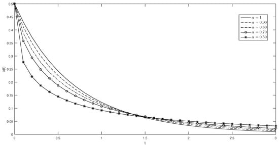
Applying the inverse conformable Laplace transform to Equation (27) and with the help of convolution operations, we obtain (see Figure 1):

$$x(t)={\displaystyle \frac{E_{\alpha }(-1,t)}{{\displaystyle \frac{t^{\alpha }}{\alpha }}+2}}$$

(28)

Example 2 (von Foerster model).

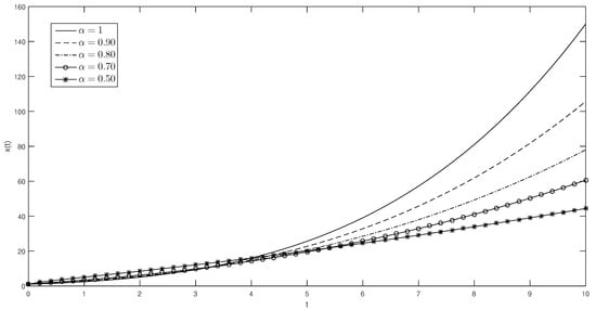
Equation (6) can however be viewed as a special case of a more general equation:

$${\mathfrak{D}}_t^{(\alpha )}x(t)=x^q(t),0<\alpha \le 1,$$

(29)

with the initial condition $x(0)=1$. The exact solution of Equation (29) is given by

$$\begin{array}{c}\hfill x(t)={exp}_q(t)={\left[1+(1-q)t\right]}_{+}^{1/(1-q)},\end{array}$$

(30)

when $\alpha =1$. Substituting Equation (21) into Equation (29), we find:

$${\mathfrak{D}}_t^{(\alpha )}z(t)=1-q,$$

(31)

subject to the initial condition $z(0)=1$. After an algebraic manipulation:

$$z(t)=1+(1-q)\frac{t^{\alpha }}{\alpha }.$$

(32)

So we get the solution as (see Figure 2)

$$x(t)={\left[1+(1-q)\frac{t^{\alpha }}{\alpha }\right]}_{+}^{\frac{1}{1-q}}={exp}_q\left(\frac{t^{\alpha }}{\alpha }\right),$$

(33)

with ${\left[y\right]}_{+}=max\left\{y,0\right\}$.

Obviously, one has:

$$\underset{q\to 1}{lim}x(t)=\underset{q\to 1}{lim}{exp}_q\left(\frac{t^{\alpha }}{\alpha }\right)=E_{\alpha }(1,t).$$

(34)

Remark 4.

In the context of nonextensive thermostatistics, the Equation (30) is the so called q-exponential function. It has become common to call the corresponding statistics ‘q-statistics’ [31]. In this work we show a generalization of the q-exponential function.

Example 3.

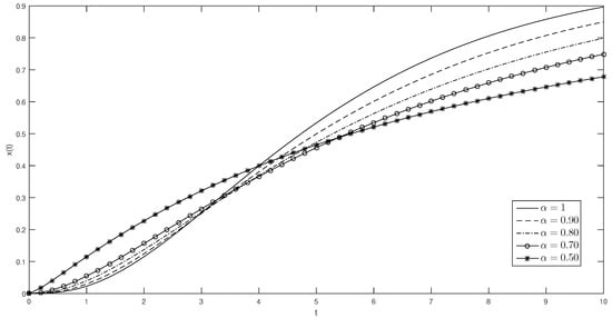
Consider the following fractional Bertalanffy-logistic differential equation:

$${\mathfrak{D}}_t^{(\alpha )}x(t)={[x(t)]}^{2/3}-x(t),0<\alpha <1,$$

(35)

subject to the initial condition $x(0)=x_0$. For $\alpha =1$, Equation (35) is the standard Bertalanffy-logistic equation:

$$x^{\prime }(t)={[x(t)]}^{2/3}-x(t),x(0)=x_0.$$

The exact solution to this problem is:

$$x(t)={\left[1+(x_0^{\frac{1}{3}}-1)e^{-\frac{t}{3}}\right]}^3.$$

(36)

The von Bertalanffy equation is a logistic model widely applied to describe the growth of different types of populations [32,33,34].

By using Equation (21) in Equation (35), we find:

$${\mathfrak{D}}_t^{(\alpha )}z(t)=\frac{1}{3}(1-z(t)),z_0=x_0^{\frac{1}{3}},0<\alpha <1.$$

(37)

Applying the conformable Laplace transform to both sides of Equation (37):

$$Z_{\alpha }(s)=\frac{1}{s}-\frac{1}{s+\frac{1}{3}}+z_0.$$

(38)

Finally, applying the inverse Laplace transform, we have (see Figure 3):

$$x(t)={\left[1+(x_0^{\frac{1}{3}}-1)e^{-\frac{t^{\alpha }}{3\alpha }}\right]}^3.$$

(39)

This can be seen when $\alpha \to 1$ in Equation (39); we get the classical solution given by Equation (36) (see Figure 3).

5. Concluding Remarks

The exact solutions of fractional differential equations play a crucial role in mathematical physics. Similarly to integer-order derivatives, by the conformable Gronwall inequality, the solutions of fractional-order equations are shown to be conformable exponentially bounded. Therefore, the validity of the Laplace transform of fractional-order equations is justified, but it requires an observation of the term forcing, so not every differential fractional equation with a constant coefficient can be solved by the method of conformable Laplace transform. We apply the conformable Laplace transform to linearized fractional-order Bernoulli equations. Analytical solutions of these models for various fractional orders and the solution of the corresponding classical equation were recovered as a particular case. We observe, in the various graphs studied, that the different values of the fractional-order of the derivative allow very different behaviors of the solution, especially in the time of convergence to the equilibrium state, which makes the model convenient to model, among others, growth phenomena.

References

- Leibniz, G.W. Letter from Hanover, Germany to Johann Bernoulli, December 28, 1695; Leibniz Mathematische Schriften; Olms-Verlag: Hildesheim, Germany, 1962; Volume 226. [Google Scholar]
- Ross, B. A brief history and exposition of the fundamental theory of fractional calculus. In Fractional Calculus and Its Applications; Springer: Berlin/Heidelberg, Germany, 1975; pp. 1–36. [Google Scholar] [CrossRef]
- Machado, J.T.; Kiryakova, V.; Mainardi, F. Recent history of fractional calculus. Commun. Nonlinear Sci. Numer. Simul. 2011, 16, 1140–1153. [Google Scholar] [CrossRef]
- Podlubny, I. Fractional Differential Equations: An Introduction to Fractional Derivatives, Fractional Differential Equations, to Methods of Their Solution and Some of Their Applications; Academic Press: Cambridge, MA, USA, 1998; Volume 198. [Google Scholar]
- Diethelm, K. The Analysis of Fractional Differential Equations: An Application-Oriented Exposition Using Differential Operators of Caputo Type; Springer: Berlin, Germany, 2010. [Google Scholar]
- Ortigueira, M.D. Fractional Calculus for Scientists and Engineers; Springer: Berlin, Germany, 2011; Volume 84. [Google Scholar]
- Baleanu, D. Fractional Calculus: Models and Numerical Methods; World Scientific: Singapore, 2012. [Google Scholar]
- Mathai, A.M. Matrix Methods and Fractional Calculus; World Scientific Publishing: Singapore, 2018. [Google Scholar]
- Yang, X.J.; Baleanu, D.; Srivastava, H.M. Local Fractional Integral Transforms and Their Applications; Academic Press: Cambridge, MA, USA, 2015. [Google Scholar]
- Haubold, H.J. Special Functions: Fractional Calculus and the Pathway for Entropy; MDPI: Basel, Switzerland, 2018. [Google Scholar]
- Oliveira, E.C.; Machado, J.A.T. A Review of Definitions for Fractional Derivatives and Integral. Math. Probl. Eng. 2014, 2014, 238459. [Google Scholar] [CrossRef]
- Tarasov, V.E. No violation of the Leibniz rule. No fractional derivative. Commun. Nonlinear Sci. Numer. Simul. 2013, 18, 2945–2948. [Google Scholar] [CrossRef]
- Khalil, R.; Al Horani, M.; Yousef, A.; Sababheh, M. A new Definition Of Fractional Derivative. J. Comput. Appl. Math. 2014, 264, 65–70. [Google Scholar] [CrossRef]
- Abdeljawad, T. On conformable fractional calculus. J. Comput. Appl. Math. 2015, 279, 57–66. [Google Scholar] [CrossRef]
- Zhao, D.; Luo, M. General conformable fractional derivative and its physical interpretation. Calcolo 2017, 54, 903–917. [Google Scholar] [CrossRef]
- Eroglu, B.I.; Avci, D.; Ozdemir, N. Optimal control problem for a conformable fractional heat conduction equation. Acta Phys. Pol. A 2017, 132, 658–662. [Google Scholar] [CrossRef]
- Pospíšil, M.; Škripková, L.P. Sturm’s theorems for conformable fractional differential equations. Math. Commun. 2016, 21, 273–281. [Google Scholar]
- Bayour, B.; Torres, D.F. Existence of solution to a local fractional nonlinear differential equation. J. Comput. Appl. Math. 2017, 312, 127–133. [Google Scholar] [CrossRef]
- Bainov, D.; Simeonov, P. Integral Inequalities and Applications; Springer: Berlin, Germany, 2013; Volume 57, pp. 89–228. ISBN 978-94-015-8034-2. [Google Scholar]
- Ames, W.F.; Pachpatte, B.G. Inequalities for Differential and Integral Equations; Elsevier: New York, NY, USA, 1997; Volume 197, ISBN 9780080534640. [Google Scholar]
- Kexue, L.; Jigen, P. Laplace transform and fractional differential equations. Appl. Math. Lett. 2011, 24, 2019–2023. [Google Scholar] [CrossRef]
- Jalilian, Y. Fractional integral inequalities and their applications to fractional differential equations. Acta Math. Sci. 2016, 36, 1317–1330. [Google Scholar] [CrossRef]
- Liang, S.; Wu, R.; Chen, L. Laplace transform of fractional order differential equations. Electron. J. Differ. Equ. 2015, 139, 1–15. [Google Scholar]
- Kohlrausch, R. Theorie des elektrischen Rückstandes in der Leidener Flasche. Ann. Phys. 1854, 167, 179–214. [Google Scholar] [CrossRef]
- Li, M. Three classes of fractional oscillators. Symmetry 2018, 10, 40. [Google Scholar] [CrossRef]
- Wuttke, J. Laplace-Fourier transform of the stretched exponential function: Analytic error bounds, double exponential transform, and open-source implementation “libkww”. Algorithms 2012, 5, 604–628. [Google Scholar] [CrossRef]
- Metzler, R.; Klafter, J. From stretched exponential to inverse power-law: fractional dynamics, Cole-Cole relaxation processes, and beyond. J. Non-Cryst. Solids 2002, 305, 81–87. [Google Scholar] [CrossRef]
- Özkan, O.; Kurt, A. The analytical solutions for conformable integral equations and integro-differential equations by conformable Laplace transform. Opt. Quantum Electron. 2018, 50, 81. [Google Scholar] [CrossRef]
- Ribeiro, F.L. A non-phenomenological model of competition and cooperation to explain population growth behaviors. Bull. Math. Biol. 2015, 77, 409–433. [Google Scholar] [CrossRef] [PubMed]
- Galanis, G.N.; Palamides, P.K. Global positive solutions of a generalized logistic equation with bounded and unbounded coefficients. Electron. J. Differ. Equ. 2003, 1–13. [Google Scholar]
- Tsallis, C. Introduction to Nonextensive Statistical Mechanics: Approaching A Complex World; Springer: Berlin, Germany, 2009. [Google Scholar]
- Renner-Martin, K.; Brunner, N.; Kühleitner, M.; Nowak, W.G.; Scheicher, K. On the exponent in the Von Bertalanffy growth model. PeerJ 2018, 6, e4205. [Google Scholar] [CrossRef] [PubMed]
- Shi, P.J.; Ishikawa, T.; Sandhu, H.S.; Hui, C.; Chakraborty, A.; Jin, X.S.; Tachiharab, K.; Li, B.L. On the 3/4-exponent von Bertalanffy equation for ontogenetic growth. Ecol. Model. 2014, 276, 23–28. [Google Scholar] [CrossRef]
- Ribeiro, F.L. An attempt to unify some population growth models from first principles. Rev. Bras. Ensino Fis. 2017, 39. [Google Scholar] [CrossRef]
© 2018 by the authors. Licensee MDPI, Basel, Switzerland. This article is an open access article distributed under the terms and conditions of the Creative Commons Attribution (CC BY) license (http://creativecommons.org/licenses/by/4.0/).