Single-Valued Neutrosophic Clustering Algorithm Based on Tsallis Entropy Maximization

Abstract

Data clustering is an important field in pattern recognition and machine learning. Fuzzy c-means is considered as a useful tool in data clustering. The neutrosophic set, which is an extension of the fuzzy set, has received extensive attention in solving many real-life problems of inaccuracy, incompleteness, inconsistency and uncertainty. In this paper, we propose a new clustering algorithm, the single-valued neutrosophic clustering algorithm, which is inspired by fuzzy c-means, picture fuzzy clustering and the single-valued neutrosophic set. A novel suitable objective function, which is depicted as a constrained minimization problem based on a single-valued neutrosophic set, is built, and the Lagrange multiplier method is used to solve the objective function. We do several experiments with some benchmark datasets, and we also apply the method to image segmentation using the Lena image. The experimental results show that the given algorithm can be considered as a promising tool for data clustering and image processing.

1. Introduction

Data clustering is one of the most important topics in pattern recognition, machine learning and data mining. Generally, data clustering is the task of grouping a set of objects in such a way that objects in the same group (cluster) are more similar to each other than to those in other groups (clusters). In the past few decades, many clustering algorithms have been proposed, such as k-means clustering [1], hierarchical clustering [2], spectral clustering [3], etc. The clustering technique has been used in many fields, including image analysis, bioinformatics, data compression, computer graphics and so on [4,5,6].

The k-means algorithm is one of the typical hard clustering algorithms that is widely used in real applications due to its simplicity and efficiency. Unlike hard clustering, the fuzzy c-means (FCM) algorithm [7] is one of the most popular soft clustering algorithms in which each data point belongs to a cluster to some degree that is specified by membership degrees in $[0,1]$, and the sum of the clusters for each of the data should be equal to one. In recent years, many improved algorithms for FCM have been proposed. There are three main ways to build the clustering algorithm. First is extensions of the traditional fuzzy sets. In this way, numerous fuzzy clustering algorithms based on the extension fuzzy sets, such as the intuitionistic fuzzy set, the Type-2 fuzzy set, etc., are built. By replacing traditional fuzzy sets with intuitionistic fuzzy set, Chaira introduced the intuitionistic fuzzy clustering (IFC) method in [8], which integrated the intuitionistic fuzzy entropy with the objective function. Hwang and Rhee suggested deploying FCM on (interval) Type-2 fuzzy set sets in [9], which aimed to design and manage uncertainty for fuzzifier m. Thong and Son proposed picture fuzzy clustering based on the picture fuzzy set (PFS) in [10]. Second, the kernel-based method is applied to improve the fuzzy clustering quality. For example, Graves and Pedrycz presented a kernel version of the FCM algorithm, namely KFCM in [11]. Ramathilagam et al. analyzed the Lung Cancer database by incorporating the hyper tangent kernel function [12]. Third, adding regularization terms to the objective function is used to improve the clustering quality. For example, Yasuda proposed an approach to FCM based on entropy maximization in [13]. Of course, we can use these together to obtain better clustering quality.

The neutrosophic set was proposed by Smarandache [14] in order to deal with real-world problems. Now, the neutrosophic set is gaining significant attention in solving many real-life problems that involve uncertainty, impreciseness, incompleteness, inconsistency and indeterminacy. A neutrosophic set has three membership functions, and each membership degree is a real standard or non-standard subset of the nonstandard unit interval $]0^{-},1^{+}[=0^{-}\cup [0,1]\cup 1^{+}$. Wang et al. [15] introduced single-valued neutrosophic sets (SVNSs), which are an extension of intuitionistic fuzzy sets. Moreover, the three membership functions are independent, and their values belong to the unit interval $[0,1]$. In recent years, the studies of SVNSs have been rapidly developing. For example, Majumdar and Samanta [16] studied the similarity and entropy of SVNSs. Ye [17] proposed correlation coefficients of SVNSs and applied them to single-valued neutrosophic decision-making problems, etc. Zhang et al. in [18] proposed a new definition of the inclusion relation of neutrosophic sets (which is also called the Type-3 inclusion relation), and a new method of ranking neutrosophic sets was given. Zhang et al. in [19] studied neutrosophic duplet sets, neutrosophic duplet semi-groups and cancelable neutrosophic triplet groups.

The clustering methods by the neutrosophic set have been studied deeply. In [20], Ye proposed a single-valued neutrosophic minimum spanning tree (SVNMST) clustering algorithm, and he also introduced single-valued neutrosophic clustering methods based on similarity measures between SVNSs [21]. Guo and Sengur introduced the neutrosophic c-means clustering algorithm [22], which was inspired by FCM and the neutrosophic set framework. Thong and Son did significant work on clustering based on PFS. In [10], a picture fuzzy clustering algorithm, called FC-PFS, was proposed. In order to determine the number of clusters, they built an automatically determined most suitable number of clusters based on particle swarm optimization and picture composite cardinality for a dataset [23]. They also extended the picture fuzzy clustering algorithm for complex data [24]. Unlike the method in [10], Son presented a novel distributed picture fuzzy clustering method on the picture fuzzy set [25]. We can note that the basic ideas of the fuzzy set, the intuitionistic fuzzy set and the SVNS are consistent in the data clustering, but there are differences in the representation of the objects, so that the clustering objective functions are different. Thus, the more adequate description can be better used for clustering. Inspired by FCM, FC-PFS, SVNS and the maximization entropy method, we propose a new clustering algorithm, the single-valued neutrosophic clustering algorithm based on Tsallis entropy maximization (SVNCA-TEM), in this paper, and the experimental results show that the proposed algorithm can be considered as a promising tool for data clustering and image processing.

The rest of paper is organized as follows. Section 2 shows the related work on FCM, IFC and FC-PFS. Section 3 introduces the proposed method, using the Lagrange multiplier method to solve the objective function. In Section 4, the experiments on some benchmark UCI datasets indicate that the proposed algorithm can be considered as a useful tool for data clustering and image processing. The last section draws the conclusions.

2. Related Works

In general, suppose dataset $D=\{X_1,X_2,\cdots ,X_n\}$ includes n data points, each of the data $X_i=\{x_{i1};x_{i2};\cdots ;x_{id}\}\in R^d$ is a d-dim feature vector. The aim of clustering is to get k disjoint clusters $\left\{C_j\right|,j=1,2,\cdots ,k\},$ satisfying $C_{j^{\prime }}{\cap }_{j^{\prime }\ne j}{C}_j=\varnothing$ and $D={\cup }_{j=1}^k{C}_j$. In the following, we will briefly introduce three fuzzy clustering methods, which are FCM, IFC and FC-PFS.

2.1. Fuzzy c-Means

The FCM was proposed in 1984 [7]. FCM is a data clustering technique wherein each data point belongs to a cluster to some degree that is specified by a membership grade. A data point $X_i$ of cluster $C_j$ is denoted by the term ${\mu }_{ij}$, which shows the fuzzy membership degree of the i-th data point in the j-th cluster. We use $V=\{V_1,V_2,\cdots ,V_k\}$ to describe the cluster centroids of the clusters, and $V_j\in R^d$ is the cluster centroid of $C_j$. The FCM is based on the minimization of the following objective function:

$$J=\sum _{i=1}^n\sum _{j=1}^k{u}_{ij}^m{\parallel x_i-V_j\parallel }^2,$$

(1)

where m represents the fuzzy parameter and $m\ge 1$. The constraints for (1) are,

$$\sum _{l=1}^k{\mu }_{il}=1,{\mu }_{ij}\in [0,1],i=1,2,\cdots ,n,j=1,2,\cdots ,k.$$

(2)

Using the Lagrangian method, the iteration scheme to calculate cluster centroids $V_j$ and the fuzzy membership degrees ${\mu }_{ij}$ of the objective function (1) is as follows:

$$V_j=\frac{{\sum }_{i=1}^n{\mu }_{ij}^m{X}_i}{{\sum }_{i=1}^n{\mu }_{ij}^m},j=1,2,\cdots ,k.$$

(3)

$${\mu }_{ij}={(\sum _{l=1}^k{(\frac{\parallel X_i-V_j\parallel }{\parallel X_i-V_l\parallel })}^{\frac{2}{m-1}})}^{-1}.i=1,2,\cdots ,n.j=1,2,\cdots ,k.$$

(4)

The iteration will not stop until it reaches the maximum iterations or $|J^{(t)}-J^{(t-1)}|<ϵ$, where $J^{(t)}$ and $J^{(t-1)}$ are the objection function value at $(t)$-th and $(t-1)$-th iterations, and $ϵ$ is a termination criterion between zero and $0.1$. This procedure converges to a local minimum or a saddle point of J. Finally, each data point is assigned to a different cluster according to the fuzzy membership value, that is $X_i$ belongs to $C_l$ if ${\mu }_{il}=max({\mu }_{i1},{\mu }_{i2},\cdots ,{\mu }_{ik})$.

2.2. Intuitionistic Fuzzy Clustering

The intuitionistic fuzzy set is an extension of fuzzy sets. Chaira proposed intuitionistic fuzzy clustering (IFC) [8], which integrates the intuitionistic fuzzy entropy with the objective function of FCM. The objective function of IFS is:

$$J=\sum _{i=1}^n\sum _{j=1}^k{\mu }_{ij}^m{\parallel X_i-V_j\parallel }^2+\sum _{j=1}^k{\pi }_j^{*}{e}^{1-{\pi }_j^{*}},$$

(5)

where ${\pi }_j^{*}=\frac{1}{n}{\sum }_{i=1}^n{\pi }_{ij}$, and ${\pi }_{ij}$ is the hesitation degree of $X_i$ for $C_j$. The constraints of IFC are similar to (2). Hesitation degree ${\pi }_{ik}$ is initially calculated using the following form:

$${\pi }_{ij}=1-{\mu }_{ij}-{(1-u_{ij}^{\alpha })}^{1/\alpha },\mathrm{where}\alpha \in [0,1],$$

(6)

and the intuitionistic fuzzy membership values are obtained as follows:

$${\mu }_{ij}^{*}={\mu }_{ij}+{\pi }_{ij},$$

(7)

where ${\mu }_{ij}^{*}({\mu }_{ij})$ denotes the intuitionistic (conventional) fuzzy membership of the i-th data in the j-th class. The modified cluster centroid is:

$$V_j=\frac{{\sum }_{i=1}^n{\mu }_{ij}^{*m}{X}_i}{{\sum }_{i=1}^n{\mu }_{ij}^{*m}},j=1,2,\cdots ,k.$$

(8)

The iteration will not stop until it reaches the maximum iterations or the difference between ${\mu }_{ij}^{*(t)}$ and ${\mu }_{ij}^{*(t-1)}$ is not larger than a pre-defined threshold $ϵ$, that is ${max}_{i,j}|{\mu }_{ij}^{*(t)}-{\mu }_{ij}^{*(t-1)}|<ϵ$.

2.3. Picture Fuzzy Clustering

In [26], Cuong introduced the picture fuzzy set (which is also called the standard neutrosophic set [27]), which is defined on a non-empty set S, $\dot{A}=\left\{\langle x,{\mu }_{\dot{A}}(x),{\eta }_{\dot{A}}(x),{\gamma }_{\dot{A}}(x)\rangle \right|x\in S\}$, where ${\mu }_{\dot{A}}(x)$ is the positive degree of each element $x\in X$, ${\eta }_{\dot{A}}(x)$ is the neutral degree and ${\gamma }_{\dot{A}}(x)$ is the negative degree satisfying the constraints,

$$\left\{\begin{array}{cc}{\mu }_{\dot{A}(x)},{\eta }_{\dot{A}(x)},{\gamma }_{\dot{A}(x)}\in [0,1],\hfill & \forall x\in S.\hfill \\ {\mu }_{\dot{A}(x)}+{\eta }_{\dot{A}(x)}+{\gamma }_{\dot{A}(x)}\le 1,\hfill & \forall x\in S.\hfill \end{array}\right.$$

(9)

The refusal degree of an element is calculated as:

$${\xi }_{\dot{A}}(x)=1-({\mu }_{\dot{A}}(x)+{\eta }_{\dot{A}}(x)+{\gamma }_{\dot{A}}(x)),\forall x\in S.$$

(10)

In [10], Thong and Son proposed picture fuzzy clustering (FC-PFS), which is related to neutrosophic clustering. The objective function is:

$$J=\sum _{i=1}^n\sum _{j=1}^k{({\mu }_{ij}(2-{\xi }_{ij}))}^m{\parallel X_i-V_j\parallel }^2+\sum _{i=1}^n\sum _{j=1}^k{\eta }_{ij}(log{\eta }_{ij}+{\xi }_{ij}).$$

(11)

where $i=1,\cdots ,n$, $j=1,\cdots ,k$. ${\mu }_{ij},{\eta }_{ij}$ and ${\xi }_{ij}$ are the positive, neutral and refusal degrees, respectively, for which each data point $X_i$ belongs to cluster $C_j$. Denote $\mu ,\eta$ and $\xi$ as the matrices whose elements are ${\mu }_{ij},{\eta }_{ij}$ and ${\xi }_{ij}$, respectively. The constraints for FC-PFS are defined as follows:

$$\left\{\begin{array}{c}{u}_{ij},{\eta }_{ij},{\xi }_{ij}\in [0,1],\hfill \\ u_{ij}+{\eta }_{ij}+{\xi }_{ij}\le 1,\hfill \\ \sum _{l=1}^k(u_{il}(2-{\xi }_{il}))=1,\hfill \\ \sum _{l=1}^k({\eta }_{il}+{\xi }_{il}/k)=1.\hfill \end{array}\right.$$

(12)

Using the Lagrangian multiplier method, the iteration scheme to calculate ${\mu }_{ij},{\eta }_{ij}$, ${\xi }_{ij}$ and $V_j$ for the model (11,12) is as the following equations:

$${\xi }_{ij}=1-({\mu }_{ij}+{\eta }_{ij})-{(1-{({\mu }_{ij}+{\eta }_{ij})}^{\alpha })}^{1/\alpha },\mathrm{where}\alpha \in [0,1],(i=1,\cdots ,n,j=1,\cdots ,k),$$

(13)

$${\mu }_{ij}=\frac{1}{{\sum }_{l=1}^k(2-{\xi }_{ij}){(\frac{\parallel X_i-V_j\parallel }{\parallel X_i-V_l\parallel })}^{\frac{2}{m-1}}},(i=1,\cdots ,n,j=1,\cdots ,k),$$

(14)

$${\eta }_{ij}=\frac{e^{-{\xi }_{ij}}}{{\sum }_{l=1}^k{e}^{-{\xi }_{il}}}(1-\frac{1}{k}\sum _{l=1}^k{\xi }_{il}),(i=1,\cdots ,n,j=1,\cdots ,k),$$

(15)

$$V_j=\frac{{\sum }_{i=1}^n{({\mu }_{ij}(2-{\xi }_{ij}))}^m{X}_i}{{\sum }_{i=1}^n{({\mu }_{ij}(2-{\xi }_{ij}))}^m},(j=1,\cdots ,k).$$

(16)

The iteration will not stop until it reaches the maximum iterations or $\parallel {\mu }^{(t)}-{\mu }^{(t-1)}\parallel +\parallel {\eta }^{(t)}-{\eta }^{(t-1)}\parallel +\parallel {\xi }^{(t)}-{\xi }^{(t-1)}\parallel <ϵ$.

3. The Proposed Model and Solutions

Definition 1.

[15] Set U as a space of points (objects), with a generic element in U denoted by u. A SVNS A in U is characterized by three membership functions, a truth membership function $T_A$, an indeterminacy membership function $I_A$ and a falsity-membership function $F_A$, where $\forall u\in U, T_A(u),I_A(u),F_A(u)\in [0,1]$. That is, $T_A:U\to [0,1],I_A:U\to [0,1]$ and $F_A:U\to [0,1]$. There is no restriction on the sum of $T_A(u),I_A(u)$ and $F_A(u)$; thus, $0\le T_A(u)+I_A(u)+F_A(u)\le 3$.

Moreover, the hesitate membership function is defined as $H_A:U\to [0,3]$ and $\forall u\in U,T_A(u)+I_A(u)+F_A(u)+H_A(u)=3$.

Entropy is a key concept in the uncertainty field. It is a measure of the uncertainty of a system or a piece of information. It is an improvement of information entropy. The Tsallis entropy [28], which is a generalization of the standard Boltzmann–Gibbs entropy, is defined as follows.

Definition 2.

[28] Let $\mathcal{X}$ be a finite set and X be a a random variable taking values $x\in \mathcal{X}$, with distribution $p(x)$. The Tsallis entropy is defined as $S_m(X)=\frac{1}{m-1}(1-{\sum }_{x\in \mathcal{X}}p{(x)}^m)$, where $m>0$ and $m\ne 1$.

For FCM, ${\mu }_{ij}$ denotes the fuzzy membership degree of $X_i$ to $C_j$, and supports ${\sum }_{j=1}^k{\mu }_{ij}=1$. From Definition 2, the Tsallis entropy of $\mu$ can be described by $S_m(\mu )={\sum }_{i=1}^n\frac{1}{m-1}(1-{\sum }_{j=1}^k{\mu }_{ij}^m)$. n being a fixed number, Yasuda [13] used the following formulary to describe the the Tsallis entropy of $\mu$:

$$S_m(\mu )=-\frac{1}{m-1}(\sum _{i=1}^n\sum _{j=1}^k{\mu }_{ij}^m-1).$$

(17)

The maximum entropy principle has been widely applied in many fields, such as spectral estimation, image restoration, error handling of measurement theory, and so on. In the following, the maximum entropy principle is applied to the single-valued neutrosophic set clustering. After the objection function of clustering is built, the maximum fuzzy entropy is used to regularize variables.

Suppose that there is a dataset D consisting of n data points in d dimensions. Let ${\mu }_{ij},{\gamma }_{ij},{\eta }_{ij}$ and ${\xi }_{ij}$ be the truth membership degree, falsity-membership degree, indeterminacy membership degree and hesitate membership degree, respectively, that each data point $X_i$ belongs to cluster $C_j$. Denote $\mu , \gamma , \eta$ and $\xi$ as the matrices, the elements of which are ${\mu }_{ij}, {\gamma }_{ij}, {\eta }_{ij}$ and ${\xi }_{ij}$, respectively, where ${\xi }_{ij}=3-{\mu }_{ij}-{\gamma }_{ij}-{\eta }_{ij}$. The single-valued neutrosophic clustering based on Tsallis entropy maximization (SVNC-TEM) is the minimization of the following objective function:

$$\begin{array}{ll}J=& \sum _{i=1}^n\sum _{j=1}^k{({\mu }_{ij}(4-{\xi }_{ij}-{\gamma }_{ij}))}^m{\parallel X_i-V_j\parallel }^2+\frac{\rho }{m-1}(\sum _{i=1}^n\sum _{j=1}^k{(u_{ij}(4-{\gamma }_{ij}-{\xi }_{ij}))}^m-1)\hfill \\ & +\sum _{i=1}^n\sum _{j=1}^k{\eta }_{ij}(log{\eta }_{ij}+{\xi }_{ij}/3),\hfill \end{array}$$

(18)

The constraints are given as follows:

$${\mu }_{ij}, {\gamma }_{ij}, {\eta }_{ij}\in [0,1],{\xi }_{ij}\in [0,3],(i=1,2,\cdots ,n,j=1,2,\cdots ,k)$$

(19)

$$\sum _{l=1}^k(u_{il}(4-{\gamma }_{il}-{\xi }_{il}))=1,(i=1,2,\cdots ,n),$$

(20)

$$\sum _{l=1}^k({\eta }_{il}+{\xi }_{il}/(3*k))=1,(i=1,2,\cdots ,n)$$

(21)

The proposed model in Formulary (18)–(21) is applied to the maximum entropy principle of the SVNS. Now, let us summarize the major points of this model as follows.

• The first term of the objection function (18) describes the weighted distance sum of each data point $X_i$ to the cluster center $V_j$. ${\mu }_{ij}$ being from the positive aspect and $(4-{\xi }_{ij}-{\gamma }_{ij})$ (four is selected in order to guarantee ${\mu }_{ij}\in [0,1]$ in the iterative calculation) from the negative aspect, denoting the membership degree for $X_i$ to $V_j$, we use ${\mu }_{ij}(4-{\xi }_{ij}-{\gamma }_{ij})$ to represent the “integrated true” membership of the i-th data point in the j-th cluster. From the maximum entropy principle, the best to represent the current state of knowledge is the one with largest entropy, so the second term of the objection function (18) describes the negative Tsallis entropy of $\mu (4-\gamma -\xi )$, which means that the minimization of (18) is the maximum Tsallis entropy. $\rho$ is the regularization parameter. If $\gamma =\eta =\xi =0$, the proposed model returns the FCM model.
• Formulary (19) guarantees the definition of the SVNS (Definition 1).
• Formulary (20) implies that the “integrated true” membership of a data point $X_i$ to the cluster center $V_j$ satisfies the sum-row constraint of memberships. For convenience, we set $T_{ij}={\mu }_{ij}(4-{\xi }_{ij}-{\gamma }_{ij})$, and $X_i$ belongs to class $C_l$ if $T_{il}=max(T_{i1},T_{i2},\cdots ,T_{ik})$.
• Equation (21) guarantees the working of the SVNS since at least one of two uncertain factors, namely indeterminacy membership degree and hesitate membership degree, always exists in the model.

Theorem 1.

The optimal solutions of the systems(18–21) are:

$$V_j=\frac{{\sum }_{i=1}^n{({\mu }_{ij}(4-{\gamma }_{ij}-{\xi }_{ij}))}^m{X}_i}{{\sum }_{i=1}^n{({\mu }_{ij}(4-{\gamma }_{ij}-{\xi }_{ij}))}^m},$$

(22)

$${\mu }_{ij}=\frac{1}{{\sum }_{l=1}^k(4-{\gamma }_{ij}-{\xi }_{ij}){(\frac{{\parallel X_i-V_j\parallel }^2+\frac{\rho }{m-1}}{{\parallel X_i-V_l\parallel }^2+\frac{\rho }{m-1}})}^{\frac{1}{m-1}}},$$

(23)

$${\gamma }_{ij}=4-{\xi }_{ij}-\frac{1}{u_{ij}{\sum }_{l=1}^k{(\frac{{\parallel X_i-V_j\parallel }^2+\frac{\rho }{m-1}}{{\parallel X_i-V_l\parallel }^2+\frac{\rho }{m-1}})}^{\frac{1}{m-1}}},$$

(24)

$${\eta }_{ij}=(1-\frac{1}{3k}\sum _{l=1}^k{\xi }_{il})\frac{e^{-{\xi }_{ij}}}{{\sum }_{l=1}^k{e}^{-{\xi }_{il}}},$$

(25)

$${\xi }_{ij}=3-{\mu }_{ij}-{\gamma }_{ij}-{\eta }_{ij}.$$

(26)

Proof. 

The Lagrangian multiplier of the optimization model (18–21) is:

$$\begin{array}{ll}J=\hfill & \sum _{i=1}^n\sum _{j=1}^k{(u_{ij}(4-{\gamma }_{ij}-{\xi }_{ij}))}^m{\parallel X_i-V_j\parallel }^2+\frac{\rho }{m-1}(\sum _{i=1}^n\sum _{j=1}^k{(u_{ij}(4-{\gamma }_{ij}-{\xi }_{ij}))}^m-1)\hfill \\ & +\sum _{i=1}^n\sum _{j=1}^k{\eta }_{ij}(log{\eta }_{ij}+{\xi }_{ij}/3)+\sum _{i=1}^n{\lambda }_i(\sum _{j=1}^C{\mu }_{ij}{(4-{\gamma }_{ij}-{\xi }_{ij})}^m)-1)\hfill \\ & +\sum _{i=1}^n{\chi }_i(\sum _{j=1}^k({\eta }_{ij}+{\xi }_{ij}/(3k))-1),\hfill \end{array}$$

(27)

where ${\lambda }_i$ and ${\chi }_i$ are Lagrangian multipliers.

In order to get $V_j$, taking the derivative of the objective function with respect to $V_j$, we have $\frac{\partial J}{\partial V_j}={\sum }_{i=1}^n{({\mu }_{ij}(4-{\gamma }_{ij}-{\xi }_{ij}))}^m(-2X_i+2V_j)$. Since $\frac{\partial J}{\partial V_j}=0$, so ${\sum }_{i=1}^n{({\mu }_{ij}(4-{\eta }_{ij}-{\xi }_{ij}))}^m(-2X_i+2V_j)=0$ $\iff {\sum }_{i=1}^n{({\mu }_{ij}(4-{\eta }_{ij}-{\xi }_{ij}))}^m{X}_i={\sum }_{i=1}^n{({\mu }_{ij}(4-{\eta }_{ij}-{\xi }_{ij}))}^m{V}_j$ $\iff V_j=\frac{{\sum }_{i=1}^n{({\mu }_{ij}(4-{\eta }_{ij}-{\xi }_{ij}))}^m{X}_i}{{\sum }_{i=1}^N{({\mu }_{ij}(4-{\eta }_{ij}-{\xi }_{ij}))}^m}$.

Similarly, $\frac{\partial J}{\partial {\mu }_{ij}}=m{\mu }_{ij}^{m-1}{(4-{\xi }_{ij}-{\eta }_{ij})}^m{\parallel X_i-V_j\parallel }^2+\frac{\rho m}{m-1}{\mu }_{ij}^{m-1}{(4-{\xi }_{ij}-{\eta }_{ij})}^m)+{\lambda }_i(4-{\xi }_{ij}-{\eta }_{ij})=0$ $\iff {\mu }_{ij}^{m-1}{(4-{\gamma }_{ij}-{\xi }_{ij})}^{m-1}(m{\parallel X_i-V_j\parallel }^2+\frac{\rho m}{m-1})+{\lambda }_i=0$ $\iff {\mu }_{ij}=\frac{1}{4-{\gamma }_{ij}-{\xi }_{ij}}{(\frac{{\lambda }_i}{m\parallel X_k-V_j{\parallel }^2+\frac{\rho m}{m-1}})}^{\frac{1}{m-1}}$.

From (20), we can get ${\sum }_{l=1}^k{(\frac{{\lambda }_i}{m{\parallel X_i-V_l\parallel }^2+\frac{m\rho }{m-1}})}^{\frac{1}{m-1}}=1$, that is ${\lambda }_i={(\frac{1}{{\sum }_{l=1}^k\frac{1}{(m{{\parallel X_i-V_l\parallel }^2+\frac{m\rho }{m-1})}^{\frac{1}{m-1}}}})}^{m-1}$, so ${\mu }_{ij}=\frac{1}{{\sum }_{l=1}^k(4-{\xi }_{ij}-{\eta }_{ij}){(\frac{{\parallel X_i-V_j\parallel }^2+\frac{\rho }{m-1}}{{\parallel X_i-V_l\parallel }^2+\frac{\rho }{m-1}})}^{\frac{1}{m-1}}}$; thus, (23) holds.

From (23), we can also get ${\mu }_{ij}(4-{\gamma }_{ij}-{\xi }_{ij})=\frac{1}{{\sum }_{l=1}^k{(\frac{{\parallel X_i-V_j\parallel }^2+\frac{\rho }{m-1}}{{\parallel X_i-V_l\parallel }^2+\frac{\rho }{m-1}})}^{\frac{1}{m-1}}}$, so ${\gamma }_{ij}=4-{\xi }_{ij}-\frac{1}{u_{ij}{\sum }_{i=1}^C{(\frac{{\parallel X_i-V_j\parallel }^2+\frac{\rho }{m-1}}{{\parallel X_i-V_k\parallel }^2+\frac{\rho }{m-1}})}^{\frac{1}{m-1}}}$; thus, (24) holds.

Similarly, $\frac{\partial L}{\partial {\eta }_{ij}}=log{\eta }_{ij}+1-{\chi }_i+{\xi }_{ij}=0$ $\iff {\eta }_{ij}=e^{(}{\chi }_i-1-{\xi }_{ij})$. From (21), we have ${\sum }_{l=1}^k{e}^{{\chi }_i-1-{\xi }_{il}}+\frac{1}{3k}{\sum }_{l=1}^k{\xi }_{il}=1$ $\iff e^{{\chi }_i-1}{\sum }_{l=1}^k{e}^{-{\xi }_{il}}=1-\frac{1}{3k}{\sum }_{l=1}^k{\xi }_{il}$ $\iff e^{{\chi }_i-1}=\frac{1-\frac{1}{3k}{\sum }_{l=1}^k{\xi }_{il}}{{\sum }_{l=1}^k{e}^{-{\xi }_{il}}}$. Therefore, we have ${\eta }_{ij}=(1-\frac{1}{3k}{\sum }_{l=1}^k{\xi }_{il})\frac{e^{-{\xi }_{ij}}}{{\sum }_{l=1}^k{e}^{-{\xi }_{il}}}$.

Finally, from Definition 1, we can get ${\xi }_{ij}=3-{\mu }_{ij}-{\gamma }_{ij}-{\eta }_{ij}$. Thus, (26) holds. ☐

Theorem 1 guarantees the convergence of the proposed method. The detailed descriptions of SVNC-TEM algorithm are presented in the following Algorithm 1:

Algorithm 1: SVNC-TEM
Input: Dataset $D=\{X_1,X_2,\cdots ,X_n\}$ (n elements, d dimensions), number of clusters k, maximal number of iterations (Max-Iter), parameters: $m,ϵ,\rho$
Output: Cluster result
1:	$t=0$;
2:	Initialize $\mu ,\gamma ,\xi ,$ satisfies Constraints (19) and (20);
3:	Repeat
4:	$t=t+1$;
5:	Update $V_j^{(t)},(j=1,2,\cdots ,k)$ using Equation (22);
6:	Update ${\mu }_{ij}^{(t)},(i=1,2,\cdots ,n,j=1,2,\cdots ,k)$ using Equation (23);
7:	Update ${\gamma }_{ij}^{(t)},(i=1,2,\cdots ,n,j=1,2,\cdots ,k)$ using Equation (24);
8:	Update ${\eta }_{ij}^{(t)},(i=1,2,\cdots ,n,j=1,2,\cdots ,k)$ using Equation (25);
9:	Update ${\xi }_{ij}^{(t)},(i=1,2,\cdots ,n,j=1,2,\cdots ,k)$ using Equation (26);
10:	Update $T_{ij}^{(t)}={\mu }_{ij}^{(t)}(4-{\gamma }_{ij}^{(t)}-{\xi }_{ij}^{(t)}),(i=1,2,\cdots ,n,j=1,2,\cdots ,k)$;
11:	Update $J^{(t)}$ using Equation (18);
12:	Until $|J^{(t)}-J^{(t-1)}|<ϵ$ or Max-Iter is reached.
13:	Assign $X_i(i=1,2,\cdots ,n)$ to the l-th class if $T_{il}=max(T_{i1},T_{i2},\cdots ,T_{ik})$.

Compared to FCM, the proposed algorithm needs additional time to calculate $\mu ,\gamma ,\eta$ and $\xi$ in order to more precisely describe the object and get better performance. If the dimension of the given dataset is d, the number of objects is n, the number of clusters is c and the number of iterations is t, then the computational complexity of the proposed algorithm is $O(dnct)$. We can see that the computational complexity is very high if d and n are large.

4. Experimental Results

In this section, some experiments are intended to validate the effectiveness of the proposed algorithm SVNC-TEM for data clustering. Firstly, we used an artificial dataset to show that SVNC-TEM can cluster well. Secondly, the proposed clustering method was used in image segmentation using an example. Lastly, we selected five benchmark datasets, and SVNC-TEM was compared to four state-of-the-art clustering algorithms, which were: k-means, FCM, IFC and FS-PFS.

In the experiments, the parameter m was selected as two and $ϵ={10}^{-5}$. The maximum iterations (Max-Iter) $=100$. The selected datasets have class labels, so the number of cluster k was known in advance. All the codes in the experiments were implemented in MATLAB R2015b.

4.1. Artificial Data to Cluster by the SVNC-TEM Algorithm

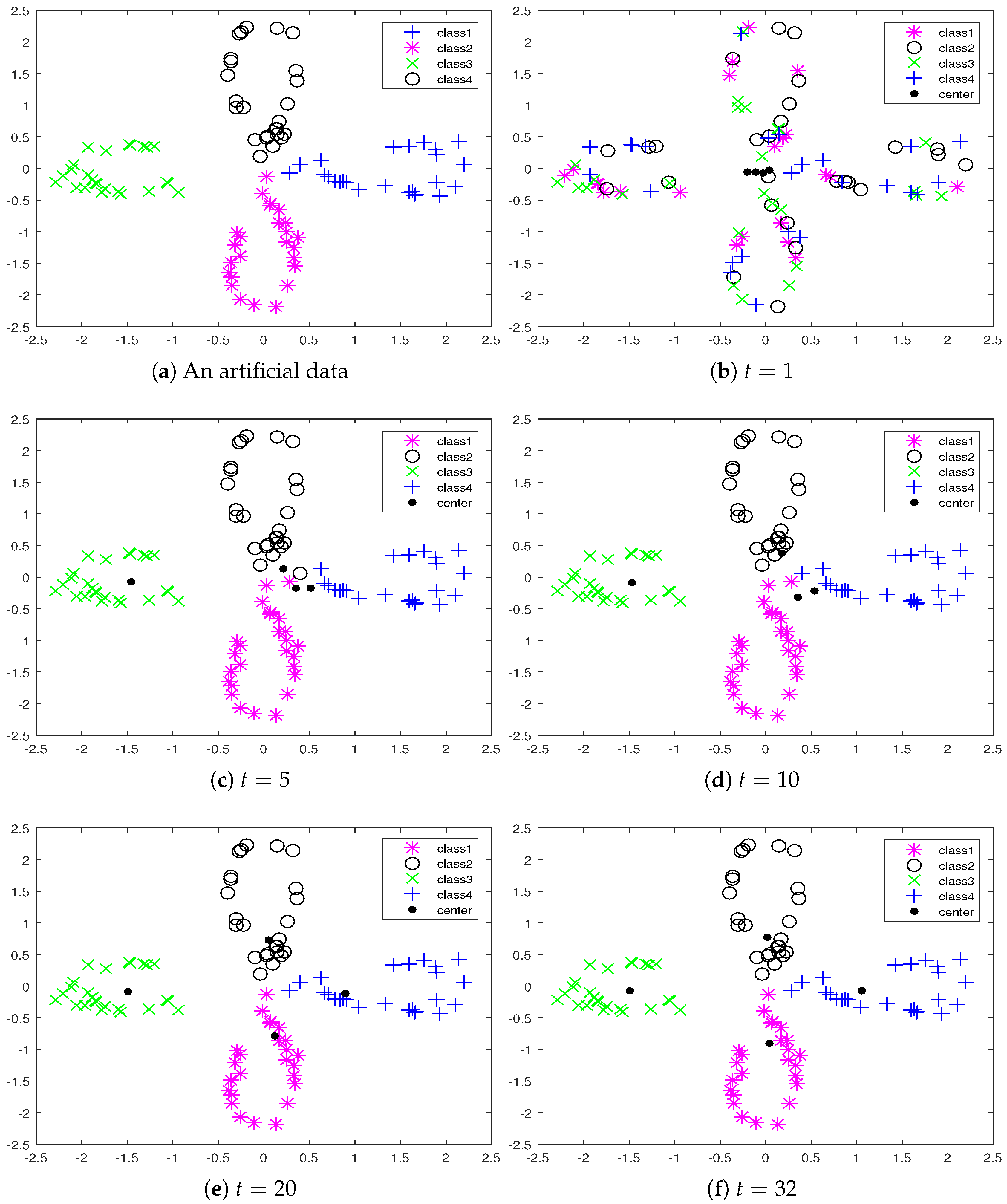
The activities of the SVNC-TEM algorithm are illustrated to cluster artificial data, which was two-dimensional data and had 100 data points, into four classes. We use an example to show the clustering process of the proposed algorithm. The distribution of data points is illustrated in Figure 1a. Figure 1b–e shows the cluster results when the number of iterations was $t=$ 1, 5, 10, 20, respectively. We can see that the clustering result was obtained when $t=20$. Figure 1f shows the final results of the clustering; the number of iterations was 32. We can see that the proposed algorithm gave correct clustering results from Figure 1.

4.2. Image Segmentation by the SVNC-TEM Algorithm

In this subsection, we use the proposed algorithm for image segmentation. As a simple example, the Lena image was used to test the proposed algorithm for image segmentation. Through this example, we wish to show that the proposed algorithm can be applied to image segmentation. Figure 2a is the original Lena image. Figure 2b shows the segmentation images when the number of clusters was $k=$ 2, and we can see that the quality of the image was greatly reduced. Figure 2c–f shows the segmentation images when the number of clusters was $k=$ 5, 8, 11 and 20, respectively. We can see that the quality of segmentation image was improved very much with the increase of the clustering number.

The above two examples demonstrate that the proposed algorithm can be effectively applied to clustering and image processing. Next, we will further compare the given algorithm to other state-of-art clustering algorithms on benchmark datasets.

4.3. Comparison Analysis Experiments

In order to verify the clustering performance, in this subsection, we experiment with five benchmark datasets of the UCI Machine Learning Repository, which are IRIS, CMC, GLASS, BALANCE and BREAST. These datasets were used to test the performance of the clustering algorithm.

Table 1. Description of the experimental datasets.

Dataset	No. of Elements	No. of Attributes	No. of Classes	Elements in Each Classes
IRIS	150	4	3	[50, 50, 50]
CMC	1473	9	3	[629, 333, 511]
GLASS	214	9	6	[29, 76, 70, 17, 13, 9]
BALANCE	625	4	3	[49, 288, 288]
BREAST	277	9	2	[81, 196]

shows the details of the characteristics of the datasets.

In order to compare the performance of the clustering algorithms, three evaluation criteria were introduced as follows.

Given one data point $X_i$, denote $p_i$ as the truth class and $q_i$ as the predicted clustering class. The clustering accuracy (ACC) measure is evaluated as follows:

$$ACC=\frac{{\sum }_{i=1}^n\delta (p_i,map(q_i))}{n},$$

(28)

where n is the total number of data points, $\delta (x,y)=1$ if $x=y$; otherwise, $\delta (x,y)=0$. $map(•)$ is the best permutation mapping function that matches the obtained clustering label to the equivalent label of the dataset. One of the best mapping functions is the Kuhn–Munkres algorithm [29]. The higher the ACC was, the better the clustering performance was.

Given two random variables X and Y, $MI(X;Y)$ is the mutual information of X and Y. $H(X)$ and $H(Y)$ are the entropies of P and Q, respectively. We use the normalized mutual information (NMI) as follows:

$$NMI(X;Y)=\frac{MI(X;Y)}{\sqrt{H(X)H(Y)}}.$$

(29)

The clustering results $\widehat{C}={\left\{{\widehat{C}}_j\right\}}_{j=1}^{\widehat{k}}$ and the ground truth classes $C={\left\{C_j\right\}}_{j=1}^k$ are regarded as two discrete random variables. Therefore, NMI is specified as follows:

$$NMI(C;\widehat{C})=\frac{{\sum }_{i=1}^{\widehat{k}}{\sum }_{j=1}^k|{\widehat{C}}_i\cap C_j|log\frac{n|{\widehat{C}}_i\cap C_j|}{|{\widehat{C}}_i||C_j|}}{\sqrt{({\sum }_{i=1}^{\widehat{k}}|{\widehat{C}}_{i}log\frac{|{\widehat{C}}_i|}{n}|)({\sum }_{j=1}^k|C_j|log\frac{|C_j|}{n})}}.$$

(30)

The higher the NMI was, the better the clustering performance was.

The Rand index is defined as,

$$RI=\frac{2(a+d)}{n(n-1)},$$

(31)

where a is the number of pairs of data points belonging to the same class in C and to the same cluster in $\widehat{C}$. d is the number of pairs of data points belonging to the different class and to the different cluster. n is the number of data points. The larger the Rand index is, the better the clustering performance is.

We did a series of experiments to indicate the performance of the proposed method for data clustering. In the experiments, we set the parameters of all approaches in the same way to make the experiments fair enough, that is for parameter $\rho$, we set $\rho =\{0.01,0.05,0.07,$$0.1,0.15,0.5,1,2,5,8,9,15,20,50\}$. For $\alpha$, we set $\alpha =\{0.1,0.2,0.3,0.4,0.5,0.6,0.7,0.8,0.9\}$. For each parameter, we ran the given method 50 times and selected the best mean value to report.

Table 2. The ACC for different algorithms on different datasets.

Dataset	k-Means	FCM	IFC	FC-PFS	SVNC-TEM
IRIS	0.8803	0.8933	0.9000	0.8933	0.9000
CMC	0.3965	0.3917	0.3958	0.3917	0.3985
GLASS	0.3219	0.2570	0.3636	0.2935	0.3681
BALANCE	0.5300	0.5260	0.5413	0.5206	0.5149
BREAST	0.6676	0.5765	0.6595	0.6585	0.6686

Bold format: the best performance.

,

Table 3. The NMI for different algorithms on different datasets.

Dataset	k-Means	FCM	IFC	FC-PFS	SVNC-TEM
IRIS	0.7514	0.7496	0.7102	0.7501	0.7578
CMC	0.0320	0.0330	0.0322	0.0334	0.0266
GLASS	0.0488	0.0387	0.0673	0.0419	0.0682
BALANCE	0.1356	0.1336	0.1232	0.1213	0.1437
BREAST	0.0623	0.0309	0.0285	0.0610	0.0797

Bold format: the best performance.

and

Table 4. The RI for different algorithms on different datasets.

Dataset	k-Means	FCM	IFC	FC-PFS	SVNC-TEM
IRIS	0.8733	0.8797	0.8827	0.8797	0.8859
CMC	0.5576	0.5582	0.5589	0.5582	0.5605
GLASS	0.5373	0.6294	0.4617	0.5874	0.4590
BALANCE	0.5940	0.5928	0.5899	0.5904	0.5999
BREAST	0.5708	0.5159	0.5732	0.5656	0.5567

Bold format: the best performance.

show the results with the different evaluation measures. In these tables, we use bold font to indicate the best performance.

We analyze the results from the dataset firstly. For IRIS dataset, the proposed method obtained the best performance for ACC, NMI and RI. For the CMC dataset, the proposed method had the best performance for ACC and RI. For the GLASS and BREAST datasets, the proposed method obtained the best performance for ACC and NMI. For the BALANCE dataset, the proposed method had the best performance for NMI and RI. On the other hand, from the three evaluation criteria, for ACC and NMI, the proposed method beat the other methods for four datasets. For RI, SVNC-TEM beat the other methods for three datasets. From the experimental results, we can see that the proposed method had better clustering performance than the other algorithms.

5. Conclusions

In the paper, we consider the truth membership degree, the falsity-membership degree, the indeterminacy membership degree and hesitate membership degree in a comprehensive way for data clustering by the single-valued neutrosophic set. We propose a novel data clustering algorithm, SVNC-TEM, and the experimental results showed that the proposed algorithm can be considered as a promising tool for data clustering and image processing. The proposed algorithm had better clustering performance than the other algorithms such as k-means, FCM, IFC and FC-PFS. Next, we will consider the proposed method to deal with outliers. Moreover, we will consider the clustering algorithm combined with spectral clustering and other clustering methods.

References

- MacQueen, J.B. Some methods for classification and analysis of multivariate observations. In Proceedings of the 5th Berkeley Symposium on Mathematical Statistics and Probability; University of California Press: Berkeley, CA, USA, 1967; pp. 281–297. [Google Scholar]
- Johnson, S.C. Hierarchical clustering schemes. Psychometrika 1967, 2, 241–254. [Google Scholar] [CrossRef]
- Ng, A.Y.; Jordan, M.I.; Weiss, Y. On spectral clustering: Analysis and an algorithm. Adv. Neural Inf. Process. Syst. 2002, 14, 849–856. [Google Scholar]
- Andenberg, M.R. Cluster Analysis for Applications; Academic Press: New York, NY, USA, 1973. [Google Scholar]
- Ménard, M.; Demko, C.; Loonis, P. The fuzzy c + 2 means: Solving the ambiguity rejection in clustering. Pattern Recognit. 2000, 33, 1219–1237. [Google Scholar]
- Aggarwal, C.C.; Reddy, C.K. Data Clustering: Algorithms and Applications; CRC Press: Boca Raton, FL, USA, 2013. [Google Scholar]
- Bezdek, J.C.; Ehrlich, R.; Full, W. FCM: The fuzzy c-means clustering algorithm. Comput. Geosci. 1984, 10, 191–203. [Google Scholar] [CrossRef]
- Chaira, T. A novel intuitionistic fuzzy C means clustering algorithm and its application to medical images. Appl. Soft Comput. 2011, 11, 1711–1717. [Google Scholar] [CrossRef]
- Hwang, C.; Rhee, F.C.H. Uncertain fuzzy clustering: interval type-2 fuzzy approach to c-means. IEEE Trans. Fuzzy Syst. 2007, 15, 107–120. [Google Scholar] [CrossRef]
- Thong, P.H.; Son, L.H. Picture fuzzy clustering: A new computational intelligence method. Soft Comput. 2016, 20, 3549–3562. [Google Scholar] [CrossRef]
- Graves, D.; Pedrycz, W. Kernel-based fuzzy clustering and fuzzy clustering: A comparative experimental study. Fuzzy Sets Syst. 2010, 161, 522–543. [Google Scholar] [CrossRef]
- Ramathilagam, S.; Devi, R.; Kannan, S.R. Extended fuzzy c-means: An analyzing data clustering problems. Clust. Comput. 2013, 16, 389–406. [Google Scholar] [CrossRef]
- Yasuda, M. Deterministic Annealing Approach to Fuzzy C-Means Clustering Based on EntropyMaximization. Adv. Fuzzy Syst. 2011, 2011, 960635. [Google Scholar] [CrossRef]
- Smarandache, F. A Unifying Field in Logics. Neutrosophy: Neutrosophic Probability, Set and Logic; American Research Press: Rehoboth, TX, USA, 1998. [Google Scholar]
- Wang, H.; Smarandache, F.; Zhang, Y.Q. Sunderraman, R. Single Valued Neutrosophic Sets. Multispace Multistruct 2010, 4, 410–413. [Google Scholar]
- Majumdar, P.; Samant, S.K. On similarity and entropy of neutrosophic sets. J. Intell. Fuzzy Syst. 2014, 26, 1245–1252. [Google Scholar]
- Ye, J. Improved correlation coefficients of single valued neutrosophic sets and interval neutrosophic sets for multiple attribute decision making. J. Intell. Fuzzy Syst. 2014, 27, 2453–2462. [Google Scholar]
- Zhang, X.; Bo, C.; Smarandache, F.; Dai, J. New Inclusion Relation of Neutrosophic Sets with Applications and Related Lattice Structure. J. Mach. Learn. Cybern. 2018, 2018, 1–11. [Google Scholar] [CrossRef]
- Zhang, X.H.; Smarandache, F.; Liang, X.L. Neutrosophic duplet semi-group and cancelable neutrosophic triplet groups. Symmetry 2017, 9, 275. [Google Scholar] [CrossRef]
- Ye, J. Single-Valued Neutrosophic Minimum Spanning Tree and Its Clustering Method. J. Intell. Syst. 2014, 23, 311–324. [Google Scholar] [CrossRef]
- Ye, J. Clustering Methods Using Distance-Based Similarity Measures of Single-Valued Neutrosophic Sets. J. Intell. Syst. 2014, 23, 379–389. [Google Scholar] [CrossRef]
- Guo, Y.; Sengur, A. NCM: Neutrosophic c-means clustering algorithm. Pattern Recognit. 2015, 48, 2710–2724. [Google Scholar] [CrossRef]
- Thong, P.H.; Son, L.H. A novel automatic picture fuzzy clustering method based on particle swarm optimization and picture composite cardinality. Knowl. Based Syst. 2016, 109, 48–60. [Google Scholar] [CrossRef]
- Thong, P.H.; Son, L.H. Picturefuzzyclusteringforcomplexdata. Eng. Appl. Artif. Intell. 2016, 56, 121–130. [Google Scholar] [CrossRef]
- Son, L.H. DPFCM: A novel distributed picture fuzzy clustering method on picture fuzzy sets. Expert Syst. Appl. 2015, 42, 51–66. [Google Scholar] [CrossRef]
- Cuong, B.C. Picture Fuzzy Sets. J. Comput. Sci. Cybern. 2014, 30, 409–420. [Google Scholar]
- Cuong, B.C.; Phong, P.H.; Smarandache, F. Standard Neutrosophic Soft Theory: Some First Results. Neutrosophic Sets Syst. 2016, 12, 80–91. [Google Scholar]
- Tsallis, C. Possible generalization of Boltzmann-Gibbs statistics. J. Stat. Phys. 1988, 52, 479–487. [Google Scholar] [CrossRef]
- Lovasz, L.; Plummer, M.D. Matching Theory; AMS Chelsea Publishing: Providence, RI, USA, 2009. [Google Scholar]
Figure 1.
The demonstration figure of the clustering process for artificial data. (a) The original data. (b–e) The clustering figures when the number of iterations 1, 5, 10, 20, respectively. (f) The final clustering result.
Figure 2.
The image segmentation for the Lena image. (a) The original Lena image. (b–f) The clustering images when the number of clusters 2, 5, 8, 11 and 20, respectively.