A New Efficient Method for the Numerical Solution of Linear Time-Dependent Partial Differential Equations

Abstract

This paper presents a new efficient method for the numerical solution of a linear time-dependent partial differential equation. The proposed technique includes the collocation method with Legendre wavelets for spatial discretization and the three-step Taylor method for time discretization. This procedure is third-order accurate in time. A comparative study between the proposed method and the one-step wavelet collocation method is provided. In order to verify the stability of these methods, asymptotic stability analysis is employed. Numerical illustrations are investigated to show the reliability and efficiency of the proposed method. An important property of the presented method is that unlike the one-step wavelet collocation method, it is not necessary to choose a small time step to achieve stability.

1. Introduction

In recent years, many kinds of wavelet bases have been utilized to solve functional equations; for example, Shannon wavelets [1], Daubechies wavelets [2] and Chebyshev wavelets [3,4]. In this paper, we utilize Legendre wavelets. Legendre wavelets are derived from Legendre polynomials [5]. These wavelets have been used in solving different kinds of functional equations such as integral equations [6,7], fractional equations [8,9], ordinary differential equations [5], partial differential equations [10,11], etc.

In solving time-dependent problems, Legendre wavelets are often used for spatial discretization. Different techniques are implemented for time discretization. In some articles, Legendre wavelets are also applied for time discretization. Therefore, the collocation points should be defined for both time and spatial variables. Also in this technique, multi-dimensional wavelets should be used to approximate required functions, which deal with large matrices and require large storage space. For example, readers can refer to [9].

There are many contexts that use collocation methods in solving functional equations. For example, Luo et al. [12] presented three collocation methods based on a family of barycentric rational interpolation functions for solving a class of nonlinear parabolic partial differential equations. Furthermore, for solving a class of fractional subdiffusion equation, Luo et al. in 2016 [13] used the quadratic spline collocation method.

Another path for time discretization uses a finite difference method. Islam et al. [10] used a fully implicit scheme, which is based on the first-order Taylor expansion. Yin et al. [11] employed the $\theta$-weighted scheme for nonlinear Klein–Sine–Gordon equations. Stability is the important point in using finite difference methods. Thus, methods that are first-order accurate in time might be inappropriate.

Here, we exploit the three-step finite element method for time discretization [14,15,16]. For the suitable differentiable function $F(t)$, these three steps are defined as follows:

$$\begin{array}{c}F(t+\frac{\Delta t}{3})=F(t)+{\displaystyle \frac{\Delta t}{3}}{\displaystyle \frac{\partial F}{\partial t}}(t),\hfill \end{array}$$

(1)

$$\begin{array}{c}F(t+\frac{\Delta t}{2})=F(t)+{\displaystyle \frac{\Delta t}{2}}{\displaystyle \frac{\partial F}{\partial t}}(t+\frac{\Delta t}{3}),\hfill \end{array}$$

(2)

$$\begin{array}{c}F(t+\Delta t)=F(t)+\Delta t{\displaystyle \frac{\partial F}{\partial t}}(t+\frac{\Delta t}{2}).\hfill \end{array}$$

(3)

It can be shown that the above equations are equivalent to the third-order Taylor expansion. Therefore, this method is third-order accurate in t. The first idea of using these three steps has been demonstrated by Jiang and Kawahara [14]. Equations (1)–(3) are usually accompanied by the Galerkin finite element method, which is known as the three-step Taylor–Galerkin method [17]. Kumar and Mehra [2] proposed a three-step wavelet Galerkin method based on the Daubechies wavelets for solving partial differential equations subject to periodic boundary conditions. In this paper, motivated and inspired by the ongoing research, we develop a new effective method, which combines the Legendre wavelets collocation method for spatial discretization and the mentioned three steps for time discretization in the numerical solution of a linear time-dependent partial differential equation subject to the Dirichlet boundary conditions. We call this method the three-step wavelet collocation method. Furthermore, we explain the asymptotic stability of the proposed method.

The organization of this paper is as follows. In Section 2, fundamental properties of the Legendre wavelets are described. The three-step wavelet collocation method is presented in Section 3. The analysis of asymptotic stability is performed in Section 4. Some numerical examples are presented in Section 5. Finally, Section 6 provides the conclusions of the study.

2. Basic Properties of Legendre Wavelets

Legendre wavelets are defined on the interval $[0,1]$ as follows [5]:

$$\begin{array}{c}\hfill \left\{\begin{array}{c}{\psi }_{l,m}(x)=\sqrt{m+\frac{1}{2}}{2}^{\frac{k+1}{2}}{L}_m(2^{k+1}x-(2l+1)),{\displaystyle \frac{l}{2^k}}\le x<{\displaystyle \frac{l+1}{2^k}}\hfill \\ 0,\mathit{otherwise}\hfill \end{array}\right.\end{array}$$

where k can assume any positive integer, $m=0,1,\cdots ,M$, $l=0,1,\cdots ,2^k-1$ and $L_m(x)$ are the well-known Legendre polynomials of order m.

A function $f(x)$ defined over $[0,1]$ can be approximated in terms of Legendre wavelets as:

$$f(x)\simeq \sum _{l=0}^{2^k-1}\sum _{m=0}^M{c}_{l,m}{\psi }_{l,m}(x)=C^T\Psi (x),$$

(4)

where:

$$\Psi (x)={[{\psi }_{0,0},{\psi }_{0,1},\cdots ,{\psi }_{0,M},{\psi }_{1,0},{\psi }_{1,1},\cdots ,{\psi }_{2^k-1,0},{\psi }_{2^k-1,1}\cdots ,{\psi }_{2^k-1,M}]}^T,$$

and $c_{l,m}=<f(x),{\psi }_{l,m}>$, in which $<.,.>$ denotes the inner product.

The derivative of the vector $\Psi (x)$ can be expressed by:

$${\displaystyle \frac{d\Psi (x)}{dx}}=D\Psi (x),$$

where D is the $2^k(M+1)$ operational matrix. Mohammadi and Hosseini obtained D and the operational matrix for the n-th derivative:

$${\displaystyle \frac{d^n\Psi (x)}{d{x}^n}}=D^n\Psi (x),$$

(5)

in [5].

3. Three-Step Wavelet Collocation Method

In this section, we explain the main structure of the three-step wavelet collocation method.

3.1. Time Discretization

Consider the following linear time-dependent partial differential equation:

$${\displaystyle \frac{\partial u}{\partial t}}=\nu ({\displaystyle \frac{{\partial }^{2}u}{\partial x^2}})+\mu u+f(x,t),$$

(6)

with the initial condition:

$$u(x,0)=g(x),0\le x\le 1$$

(7)

and boundary conditions:

$$\begin{array}{c}u(0,t)=h_0(t),\hfill \end{array}$$

(8)

$$\begin{array}{c}u(1,t)=h_1(t),t\ge 0.\hfill \end{array}$$

(9)

Assume that $n\ge 0$ and $\Delta t$ denote the time step such that $t_n=n\Delta t,n=0,1,\cdots N_t$. By using the Taylor expansion, the value of the function $u(x,t)$ at the time $t_{n+1}$ can be expressed as follows:

$$\begin{array}{cc}\hfill u^{n+1}=u^n& +\Delta t{({\displaystyle \frac{\partial u}{\partial t}})}^n+{\displaystyle \frac{{(\Delta t)}^2}{2}}{({\displaystyle \frac{{\partial }^{2}u}{\partial t^2}})}^n+{\displaystyle \frac{{(\Delta t)}^3}{6}}{({\displaystyle \frac{{\partial }^{3}u}{\partial t^3}})}^n+\mathbf{o}[{(\Delta t)}^4],\hfill \end{array}$$

(10)

where the symbols $u^n$ and ${({\displaystyle \frac{\partial u}{\partial t}})}^n$ represent $u(x,t_n)$ and ${\displaystyle \frac{\partial u}{\partial t}}(x,t_n)$, respectively.

We can use the first-order Taylor expansion for time discretization and Legendre wavelets for spatial discretization [10]. We call this method the one-step wavelet collocation method. In addition, the time derivative in the given differential equations is approximated by Euler’s formula:

$${({\displaystyle \frac{\partial u}{\partial t}})}^n={\displaystyle \frac{u(x,t_{n+1})-u(x,t_n)}{\Delta t}}+\mathbf{o}\left[(\Delta t)\right],$$

and therefore, we have semi-discrete equation:

$$u^{n+1}=u^n+\Delta t{({\displaystyle \frac{\partial u}{\partial t}})}^n.$$

The three-step Taylor method for time discretization is derived by applying a factorization process to the right side of Equation (10) as follows:

$$\begin{array}{c}\hfill \left(\mathbf{I}+\Delta t{\displaystyle \frac{\partial }{\partial t}}[\mathbf{I}+{\displaystyle \frac{\Delta t}{2}}{\displaystyle \frac{\partial }{\partial t}}[\mathbf{I}+{\displaystyle \frac{\Delta t}{3}}{\displaystyle \frac{\partial }{\partial t}}]]\right)u^n=u^n+\Delta t{\displaystyle \frac{\partial }{\partial t}}[u^n+{\displaystyle \frac{\Delta t}{2}}{\displaystyle \frac{\partial }{\partial t}}[u^n+{\displaystyle \frac{\Delta t}{3}}{({\displaystyle \frac{\partial u}{\partial t}})}^n]].\end{array}$$

(11)

where the symbol $\mathbf{I}$ is the identity operator.

Now, using Equation (11) and employing a new notation, the three-step Taylor method is obtained as follows:

$$\begin{array}{cc}\hfill u^{n+\frac{1}{3}}& =u^n+{\displaystyle \frac{\Delta t}{3}}{({\displaystyle \frac{\partial u}{\partial t}})}^n\hfill \end{array}$$

(12)

$$\begin{array}{cc}\hfill u^{n+\frac{1}{2}}& =u^n+{\displaystyle \frac{\Delta t}{2}}{({\displaystyle \frac{\partial u}{\partial t}})}^{n+\frac{1}{3}}\hfill \end{array}$$

(13)

$$\begin{array}{cc}\hfill u^{n+1}& =u^n+\Delta t{({\displaystyle \frac{\partial u}{\partial t}})}^{n+\frac{1}{2}}.\hfill \end{array}$$

(14)

It should be noted that $u^{n+\frac{1}{3}}$, $u^{n+\frac{1}{2}}$ and $u^{n+1}$ represent the computed solution at time level ($t_n+{\displaystyle \frac{\Delta t}{3}}$), ($t_n+{\displaystyle \frac{\Delta t}{2}}$) and ($t_n+\Delta t$), respectively.

3.2. Spatial Discretization

After time discretization, the spatial derivatives of $u(x,t)$ are approximated by Legendre wavelets. The collocation method is utilized in this part. Let the unknown solution $u(x,t_n)$ be expanded by:

$$\begin{array}{c}\hfill u(x,t_n)\simeq u^n=\sum _{l=0}^{2^k-1}\sum _{m=0}^M{c}_{l,m}^n{\psi }_{l,m}(x)={(C^n)}^T\Psi (x).\end{array}$$

(15)

According to Equation (15), we use only one-dimensional Legendre wavelets to approximate the solution. The solution dependence on the time variable is specified by the coefficient $c_{l,m}^n$. In other words, the vector coefficient $C^n$ is calculated at time $t_n$. Therefore, the approximation solution at time $t_{n+\frac{1}{3}}$ can be written as follows:

$$u^{n+\frac{1}{3}}={(C^{n+\frac{1}{3}})}^T\Psi (x).$$

(16)

We can also approximate $f(x,t)$ at time $t_n$ as:

$$f(x,t_n)\simeq f^n={(F^n)}^T\Psi (x),$$

(17)

where the vector ${(F^n)}^T$ is given by Equation (4) at time $t_n$.

Substituting Equation (6) into Equation (12) results in:

$$\begin{array}{cc}\hfill u^{n+\frac{1}{3}}=u^n& +{\displaystyle \frac{\Delta t}{3}}\left(\nu {({\displaystyle \frac{{\partial }^{2}u}{\partial x^2}})}^n+\mu u^n+f(x,t_n)\right).\hfill \end{array}$$

(18)

Now, by using the operation matrix of the derivative and Equation (5), we have:

$$\begin{array}{c}\hfill {\displaystyle \frac{{\partial }^{2}u}{\partial x^2}}(x,t_n)\simeq \sum _{l=0}^{2^k-1}\sum _{m=0}^M{c}_{l,m}^n{\displaystyle \frac{{\partial }^2{\psi }_{l,m}}{\partial x^2}}(x)={(C^n)}^T{D}^2\Psi (x).\end{array}$$

(19)

Then, substituting Equations (15)–(17) and (19) into Equation (18) yields:

$$\begin{array}{c}\hfill {(C^{n+\frac{1}{3}})}^T\Psi (x)={(C^n)}^T\Psi (x)+{\displaystyle \frac{\Delta t}{3}}\left(\nu {(C^n)}^T{D}^2\Psi (x)+\mu {(C^n)}^T\Psi (x)+{(F^n)}^T\Psi (x)\right).\end{array}$$

(20)

By using boundary conditions and Equation (16), the following equalities are satisfied:

$$\begin{array}{cc}\hfill h_0(t_{n+\frac{1}{3}})& =u(0,t_{n+\frac{1}{3}})\simeq {(C^{n+\frac{1}{3}})}^T\Psi (0),\hfill \end{array}$$

(21)

$$\begin{array}{cc}\hfill h_1(t_{n+\frac{1}{3}})& =u(1,t_{n+\frac{1}{3}})\simeq {(C^{n+\frac{1}{3}})}^T\Psi (1).\hfill \end{array}$$

(22)

Considering the initial Condition (7), we have:

$$g(x)=u(x,t_0)\simeq u^0={(C^0)}^T\Psi (x)$$

(23)

By substituting Equation (20) in $(2^k(M+1)-2)$ Gauss–Legendre points ${\left\{x_i\right\}}_{i=1}^{2^k(M+1)-2}$ and using Equations (21) and (22), we can obtain a linear system of equations with $2^k(M+1)$ unknown variables, $c_{l,m}^{n+\frac{1}{3}}$, which can be written in matrix form:

$$A{C}^{n+\frac{1}{3}}=B,$$

(24)

where A and B are $2^k(M+1)\times 2^k(M+1)$ and $2^k(M+1)\times 1$ matrices, respectively. Since the vector $C^0$ is obtained from Equation (23), all entries of B are known.

The above system of linear equations can be solved by numerical methods. Here, for square matrix A, we use $LU$ decomposition to solve the linear System (24) with partial pivoting. In this method, the square matrix A can be decomposed into two square matrices L and U such that $A=LU$, where U is an upper triangular matrix formed as a result of applying the Gauss elimination method on A, and L is a lower triangular matrix with diagonal elements being equal to one. Solving the system $A{C}^{n+\frac{1}{3}}=B$ is then equivalent to solving the two simpler systems $Ly=B$ and $U{C}^{n+\frac{1}{3}}=y$. The first system can be solved by forward substitution, and the second system can be solved by backward substitution. Solving the linear system with triangular matrices makes it easy to do calculations in the process of finding the solution. Since the Gaussian elimination can produce bad results for small pivot elements, we adopt the partial pivoting strategy. In this strategy, when we are choosing the pivot element on the diagonal at position $a_{ii}$, locate the element in column i at or below the diagonal that has the largest absolute value, and make it as the pivot at that step by interchanging two rows. Applying this strategy to our matrix avoids any distortion due to the pivots being small. For more details, readers can refer to [18,19].

After solving this system and determining $C^{n+\frac{1}{3}}$, we exploit Equation (13) to find $C^{n+\frac{1}{2}}$. In addition, there is a similar process that results in:

$$\begin{array}{c}\hfill {(C^{n+\frac{1}{2}})}^T\Psi (x_i)={(C^n)}^T\Psi (x_i)+{\displaystyle \frac{\Delta t}{2}}\left(\nu {(C^{n+\frac{1}{3}})}^T{D}^2\Psi (x_i)+\mu {(C^{n+\frac{1}{3}})}^T\Psi (x_i)+{(F^{n+\frac{1}{3}})}^T\Psi (x_i)\right),\end{array}$$

(25)

and:

$$\begin{array}{cc}\hfill h_0(t_{n+\frac{1}{2}})& =u(0,t_{n+\frac{1}{2}})\simeq {(C^{n+\frac{1}{2}})}^T\Psi (0),\hfill \end{array}$$

(26)

$$\begin{array}{cc}\hfill h_1(t_{n+\frac{1}{2}})& =u(1,t_{n+\frac{1}{2}})\simeq {(C^{n+\frac{1}{2}})}^T\Psi (1),\hfill \end{array}$$

(27)

where ${\left\{x_i\right\}}_{i=1}^{2^k(M+1)-2}$ are the same collocation points used in the previous step.

A matrix form of Equations (25)–(27) can be displayed as:

$$P{C}^{n+\frac{1}{2}}=Q,$$

where the dimension of the square matrix P and column vector Q is $2^k(M+1)$. Since the vector $C^{n+\frac{1}{3}}$ is obtained from the previous step, all entries of Q are known. Similarly, we use $LU$ decomposition to solve the above system.

Finally, by implementing similar analysis in the two previous steps, using Equation (14) with boundary conditions and exploiting $C^{n+\frac{1}{2}}$, the vector $C^{n+1}$ can be specified in each step for $n=0,1,2,\cdots$. Therefore, we can obtain the numerical solution, $u(x,t_n)$, in any time $t=t_n$.

4. Stability Analysis

For stability analysis, we use the asymptotic (or absolute) stability of a numerical method, which is defined in [20]. In a numerical scheme, when we fix the final time $t=n\Delta t$ and let $n\to \infty$, we want the corresponding numerical solution to remain bounded; a scheme satisfying this property is called stable. Therefore, a stability analysis needs a restriction on the mesh size $\Delta t$. In practice, we can only choose a finite and proper mesh size. It is then important to study the region of absolute stability in order to to choose the proper mesh size in practical computation.

Let us start from the typical evolution equation:

$$\begin{array}{c}\hfill {\displaystyle \frac{\partial u}{\partial t}}=f(u,t),t>0\\ \hfill u(0)=0,\end{array}$$

where the non-linear operator f contains the spatial part of the partial differential equation. Let us abbreviate $u(x_j,t_n)$ by $u_j^n$. We shall approximate $u_j^n$ by $U_j^n$. Following the general formulation of the proposed method, the semi-discrete version is:

$$Q_j{\displaystyle \frac{d{u}_j}{dt}}=Q_j{f}_j(u_j),$$

where $u_j$ is the spectral approximation to u, $f_j$ denotes the spectral approximation to the operator f and $Q_j$ is the projection operator, which characterizes the scheme. Let us set $U(t)=Q_j{u}_j(t)$. Then, the previous discrete problem can be written in the form:

$${\displaystyle \frac{dU}{dt}}=F(U).$$

(28)

As is often done, we confine our discussion of time-discretizations to the linearized version of (28):

$${\displaystyle \frac{dU}{dt}}=LU$$

(29)

where L is the diagonalizable matrix resulting from the implementation of spectral method on the spatial variable of the partial differential equation.

According to different contexts, the time discretization is said to be stable if $U^n$, the computed solution at the time $t_n=n\Delta t$, has been upper bounded, i.e., there exists a constant M such that:

$$\parallel U^n\parallel ⩽M.$$

(30)

In many problems, the solution is bounded in some norm for all $t>0$. In these cases, a method that produces the exponential growth allowed by Estimate (30) is not practical for long-time integrations. For such problems, the notion of asymptotic (or absolute) stability is useful.

Definition 1.

The region of absolute stability of a numerical method is defined for the scalar model problem:

$${\displaystyle \frac{dU}{dt}}=\lambda U$$

to be the set of all $\lambda \Delta t$ such that $\parallel U^n\parallel$ is bounded as $t\to \infty$ [20].

Finally, we say that a numerical method is asymptotically stable for a particular problem if, for sufficiently small $\Delta t$, the product of $\Delta t$ times every eigenvalue of L lies within the region of absolute stability. In the following items, we summarize some remarkable characteristics of absolute stability [21]:

1.

An absolutely stable method is one that generates a solution $u^n$ that tends to zero as $t_n$ tends to infinity,

2.

A method is said to be A-stable, if it is absolutely stable for any possible choice of the time-step, $\Delta t$, otherwise a method is called conditionally stable.

3.

Absolutely stable methods keep the perturbation controlled,

4.

The analysis of absolute stability for the linear model problem can be exploited to find stability conditions on the time step when considering some nonlinear problems.

Since the three-step Equations (12)–(14) are equivalent to the third-order Taylor expansion, to demonstrate the stability region and achieve the stability condition, we use Equation (10). For simplicity, consider Equation (6), where $\mu =0$ and $f(x,t)=0$. Then, successive differentiations of the obtained equation indicate that:

$$\begin{array}{cc}\hfill {\displaystyle \frac{{\partial }^{2}u}{\partial t^2}}& ={\nu }^2{\displaystyle \frac{{\partial }^{4}u}{\partial x^4}},\hfill \end{array}$$

(31)

$$\begin{array}{cc}\hfill {\displaystyle \frac{{\partial }^{3}u}{\partial t^3}}& ={\nu }^2{\displaystyle \frac{{\partial }^4}{\partial x^4}}({\displaystyle \frac{u^{n+1}-u^n}{\Delta t}})+\mathbf{o}\left[(\Delta t)\right].\hfill \end{array}$$

(32)

In Equation (32), we use Euler’s formula to avoid the third-order space derivatives, as it is used in the finite element context [22]. By rearranging Equation (10) and substitution of Equations (31) and (32), we have the semi-discrete equation:

$$\begin{array}{cc}\hfill (I& -{\displaystyle \frac{{\nu }^2\Delta t^2}{6}}{\displaystyle \frac{{\partial }^4}{\partial x^4}})({\displaystyle \frac{u^{n+1}-u^n}{\Delta t}})=\nu ({\displaystyle \frac{{\partial }^{2}u}{\partial x^2}}{)}^n+{\displaystyle \frac{({\nu }^2\Delta t)}{2}}({\displaystyle \frac{{\partial }^{4}u}{\partial x^4}}{)}^n.\hfill \end{array}$$

(33)

After applying the wavelet collection method, Equation (33) transforms into the following equation:

$$({\displaystyle \frac{dC}{dt}}{)}^n\simeq ({\displaystyle \frac{C^{n+1}-C^n}{\Delta t}})=A^{-1}B{C}^n,$$

(34)

where:

$$\begin{array}{c}\hfill A=\left((I-{\displaystyle \frac{{\nu }^2\Delta t^2}{6}}{D}^4){(\Psi (x_i))}^T\right),\\ \hfill B=\left((\nu D^2+{\displaystyle \frac{{\nu }^2\Delta t}{2}}{D}^4){(\Psi (x_i))}^T\right),\end{array}$$

and ${\left\{x_i\right\}}_{i=1}^{2^k(M+1)}$ are the collocation and boundary points. Here, the matrix L, which is introduced in Equation (29), is defined as $L=A^{-1}B$.

There is a similar process to the one-step method. Lambert provided an explanation for how to draw the stability region. Readers can refer to [23], Chapter 3. Briefly, we can plot the region of absolute stability, $R_L$, by the meaning of the first and second characteristic polynomials. If we set, $\widehat{h}=\lambda \Delta t$, the region of absolute stability is a function of the method and the complex parameter $\widehat{h}$ only, so that we are able to plot the region $R_L$ in the complex $\widehat{h}$-plane.

First of all, we can write Equation (34) as a usual linear multi-step method given by:

$$\sum _{j=0}^k{\alpha }_j{C}^{n+j}=\Delta t\sum _{j=0}^k{\beta }_{j}L(C^{n+j}),$$

(35)

where k is the number of steps required for the method, and ${\alpha }_j$ and ${\beta }_j$ are constants subject to the conditions:

$${\alpha }_k=1,|{\alpha }_0|+|{\beta }_0|\ne 0.$$

According to Equations (34) and (35), we have:

$$k=1,{\alpha }_0=-1,{\alpha }_1=1,{\beta }_0=1,{\beta }_1=0.$$

(36)

Afterward, the first and second characteristic polynomials are defined as follows, respectively:

$$\begin{array}{c}\hfill \rho (\xi )=\sum _{j=0}^k{\alpha }_j{\xi }^j,\\ \hfill \sigma (\xi )=\sum _{j=0}^k{\beta }_j{\xi }^j,\end{array}$$

where $\xi \in \mathbb{C}$ is a dummy variable. Using the values of k and ${\{{\alpha }_j,{\beta }_j\}}_{j=0}^1$ in (36), for the proposed method, we have:

$$\rho (\xi )=\xi -1,\sigma (\xi )=1.$$

Then, we plot the boundary of $R_L$, which consists of the contour $\partial R_L$. The contour $\partial R_L$ in the complex $\widehat{h}$-plane is defined by the requirement that for all $\widehat{h}\in \partial R_L$, one of the roots of $\pi (r,\widehat{h}):=\rho (r)-\widehat{h}\sigma (r)$ has modulus one, that is, it is of the form $r=exp(i\theta )$. Thus, for all $\widehat{h}$ in $\partial R_L$, the identity:

$$\pi (exp(i\theta ),\widehat{h})=\rho (exp(i\theta ))-\widehat{h}\sigma (exp(i\theta ))=0,$$

must hold. This equation is readily solved for $\widehat{h}$, and we have that the locus of $\partial R_L$ is given by:

$$\widehat{h}=\widehat{h}(\theta )={\displaystyle \frac{\rho (exp(i\theta ))}{\sigma (exp(i\theta ))}}=exp(i\theta )-1.$$

(37)

Finally, we use (37) to plot $\widehat{h}(\theta )$ for a range of $\theta \in [0,2\pi ]$ and link consecutive plotted points by straight lines to get a representation of $\partial R_L$.

Therefore, according to Lambert’s book and the above explanations, the stability region of the three-step and one-step wavelet collocation methods is the circle with center $(-1,0)$ and radius one. Therefore, these methods will be stable if the eigenvalues of the corresponding system and $\Delta t$ satisfy $Re({\lambda }_j\Delta t)\in [-2,0]$.

5. Numerical Examples

In this section, some numerical examples in the form of Equation (6) with initial and boundary Conditions (7)–(9) are discussed. The error function is defined as the maximum error $L_{\infty }$:

$$\begin{array}{c}\hfill L_{\infty }=\underset{1\le i\le 2^k(M+1)}{max}|u_{exact}(x_i,t_n)-\overline{u}(x_i,t_n)|,\end{array}$$

where $\overline{u}$ is the approximate solution, which is obtained by the proposed method and ${\left\{x_i\right\}}_{i=1}^{2^k(M+1)}$ are the Gauss–Legendre and boundary points. All programs have been performed in MATLAB 2016.

In general, the numerical results are sensitive to the selection of parameters such as time step $\Delta t$, final time t and parameters of wavelet order M and k. In the following examples, we choose $t=0.5$. Although the one-step wavelet collocation method needs less calculation, the three-step wavelet collocation method is more successful in finding the numerical solution. Furthermore, we compare our method with the three-step method proposed in [17]. They used the finite element method with standard linear interpolation functions for spatial discretization and the same three-step formula for time discretization. Numerical results show that utilizing Legendre wavelets with these three steps gives higher accuracy.

Example 1.

Consider Equation (6) with $\nu =1/{\pi }^2$, $\mu =-3$, $f(x,t)=3$, $g(x)=1+sin(\pi x)$, $h_0(t)=1$ and $h_1(t)=1$. The exact solution of this problem is $u_{exact}(x,t)=1+e^{-4t}sin(\pi x)$ [3].

Numerical results for $M=6$ and $M=8$ are reported in

Table 1. The $L_{\infty }$ error of Example 1 in $M=6$.

k	$\mathbf{\Delta }\mathit{t}$	Method in [17]	One-Step Method	Three-Step Method
2	$0.001$	2.1847$\times {10}^{-3}$	1.8061$\times {10}^{-4}$	$1.5183\times {10}^{-4}$
2	$0.01$	unstable	unstable	$1.5179\times {10}^{-4}$
3	$0.0001$	$1.6291\times {10}^{-3}$	$1.3751\times {10}^{-4}$	$1.0575\times {10}^{-4}$
3	$0.003$	unstable	unstable	$1.0510\times {10}^{-4}$

and

Table 2. The $L_{\infty }$ error of Example 1 in $M=8$.

k	$\mathbf{\Delta }\mathit{t}$	Method in [17]	One-Step Method	Three-Step Method
1	$0.001$	$2.3446\times {10}^{-3}$	$9.0287\times {10}^{-5}$	$2.1781\times {10}^{-5}$
1	$0.006$	$2.3325\times {10}^{-3}$	unstable	$1.5179\times {10}^{-4}$
2	$0.001$	$1.1569\times {10}^{-3}$	$6.5330\times {10}^{-5}$	$2.4159\times {10}^{-5}$
2	$0.005$	$1.1531\times {10}^{-3}$	unstable	$1.8234\times {10}^{-5}$

, respectively. The first two rows of Table 1 show the obtained results for $k=2$. As can be seen from these rows, a change in the length of the time step makes the one-step method fail to find an approximate solution. In other words, the one-step method is unstable for $\Delta t=0.01$, while the three-step method gives high accuracy. There is a similar analysis for other parameters.

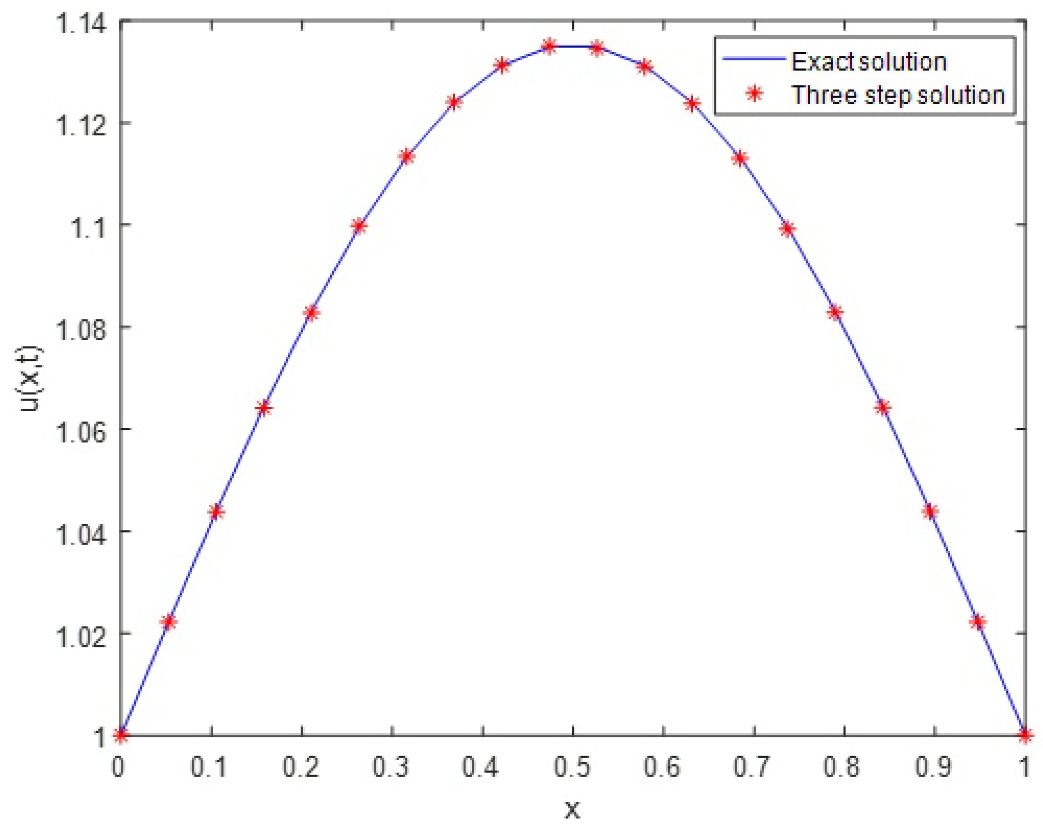
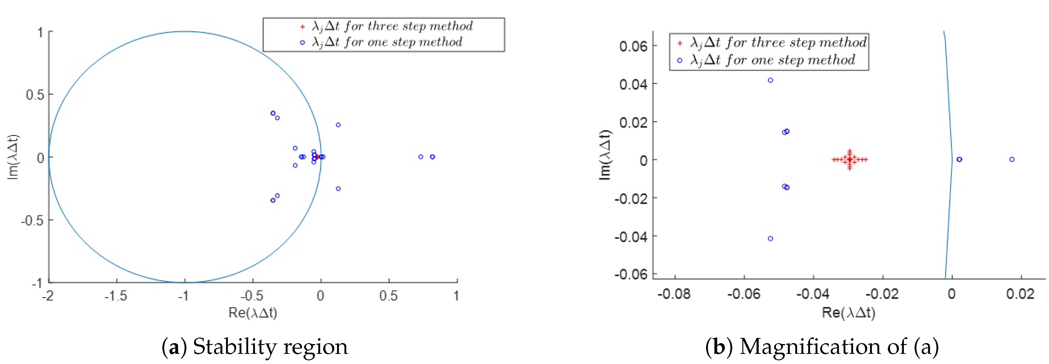
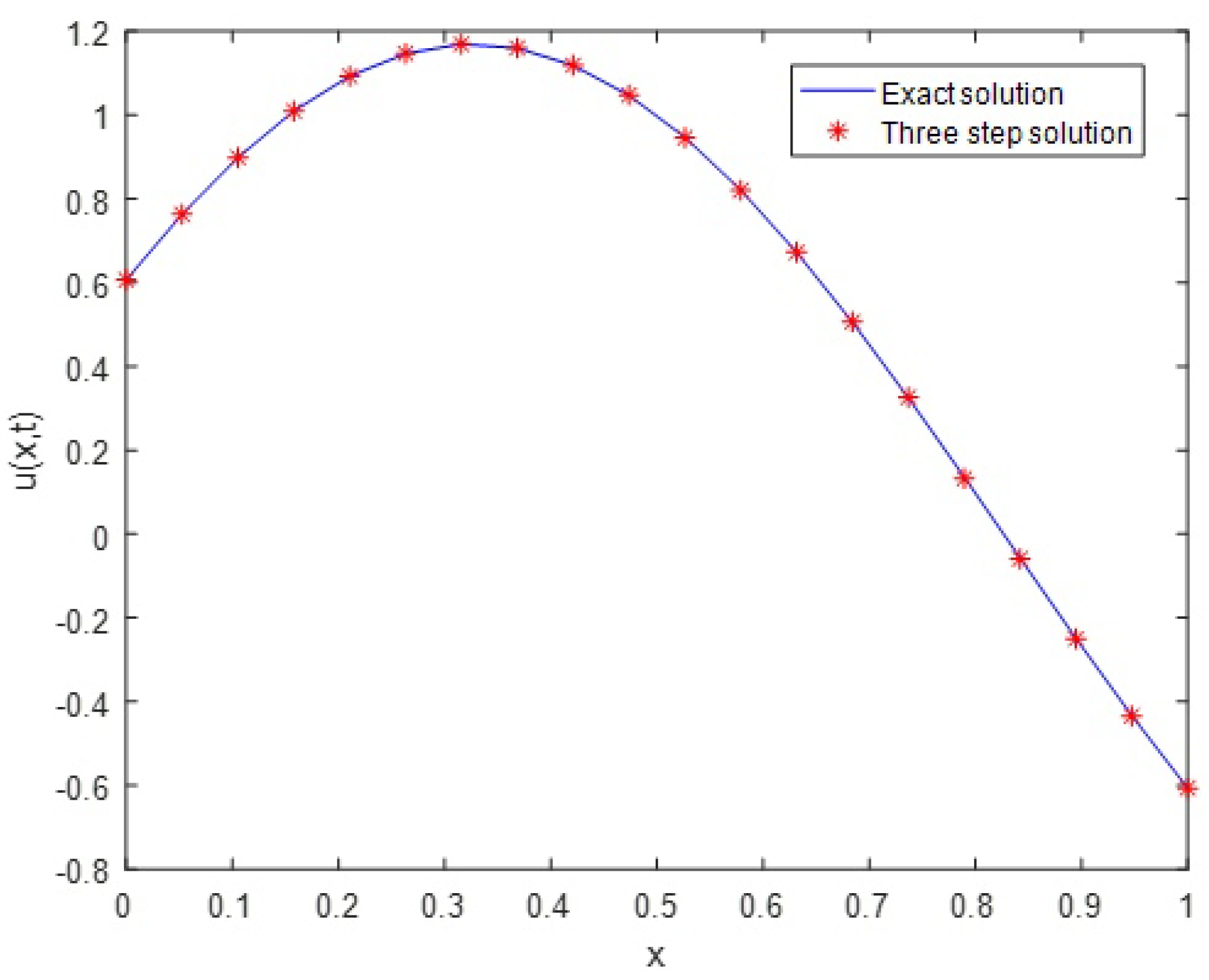
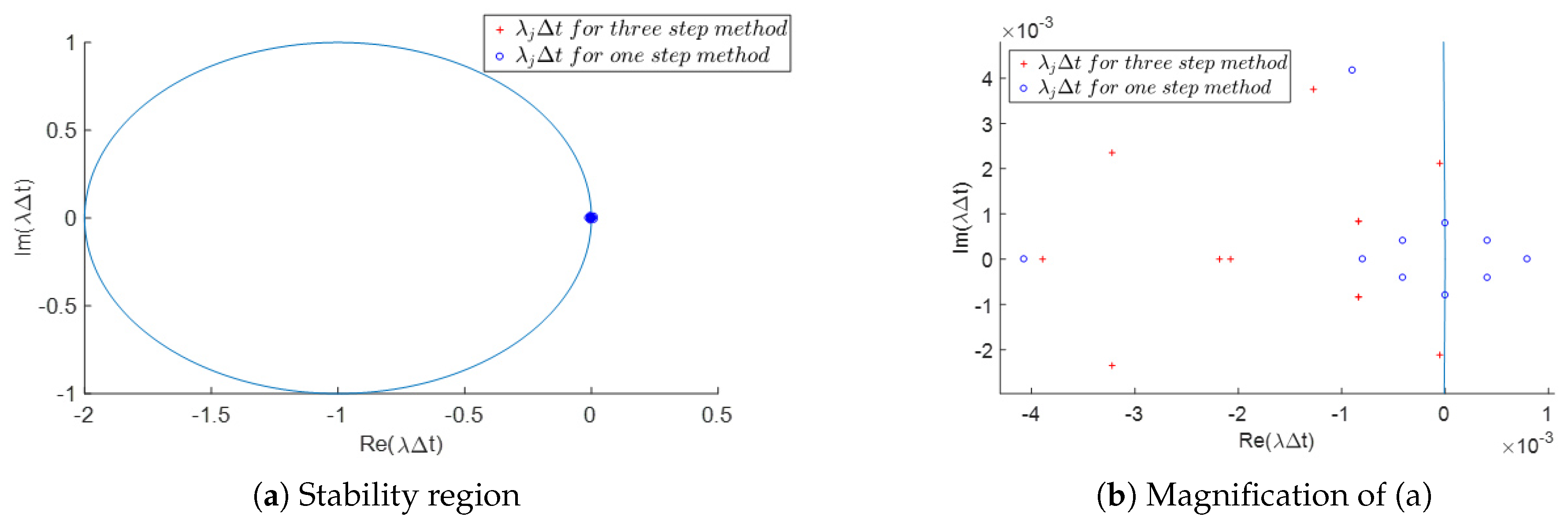
The exact and three-step approximate solutions of $u(x,t)$ are shown in Figure 1, where $M=8$ and $k=2$. Figure 2 shows the absolute stability region based on the three-step and one-step methods with the position of ${\lambda }_j\Delta t$, where ${\left\{{\lambda }_j\right\}}_{j=1}^{2^k(M+1)}$ are the eigenvalues of corresponding matrix L. This figure is drawn for $M=6$ and $\Delta t=0.01$. As can be seen in this figure, there are some eigenvalues for the one-step method with $Re({\lambda }_j\Delta t)\notin [-2,0]$; however, the stability region of the three-step method includes all ${\{{\lambda }_j\Delta t\}}_{j=1}^{2^k(M+1)}$. Therefore, the one-step method is not stable for $\Delta t=0.01$, while the three-step method is stable.

Example 2.

In this example, we consider Equation (6) with $\nu =1/{\pi }^2$, $\mu =-4$, $f(x,t)=0$, $g(x)=sin(\pi x)$, $h_0(t)=0$ and $h_1(t)=0$. The exact solution of this problem is $u_{exact}(x,t)=e^{-5t}sin(\pi x)$ [3].

Table 3. The $L_{\infty }$ error of Example 2 in $M=8$.

k	$\mathbf{\Delta }\mathit{t}$	Method in [17]	One-Step Method	Three-Step Method
1	$0.001$	$8.6091\times {10}^{-4}$	$7.3255\times {10}^{-5}$	$3.0210\times {10}^{-5}$
1	$0.006$	$8.5713\times {10}^{-4}$	unstable	$3.0028\times {10}^{-5}$
2	$0.001$	$7.2449\times {10}^{-4}$	$5.2636\times {10}^{-5}$	$1.6575\times {10}^{-5}$
2	$0.0016$	$7.2280\times {10}^{-4}$	unstable	$1.6528\times {10}^{-5}$

gives the comparison between the three-step wavelet collocation method and one-step wavelet collocation method for $M=8$. We can see from this table that the one-step wavelet collocation method tends to be unstable with a small change in time length. However, the three-step method keeps its stability for bigger $\Delta t$.

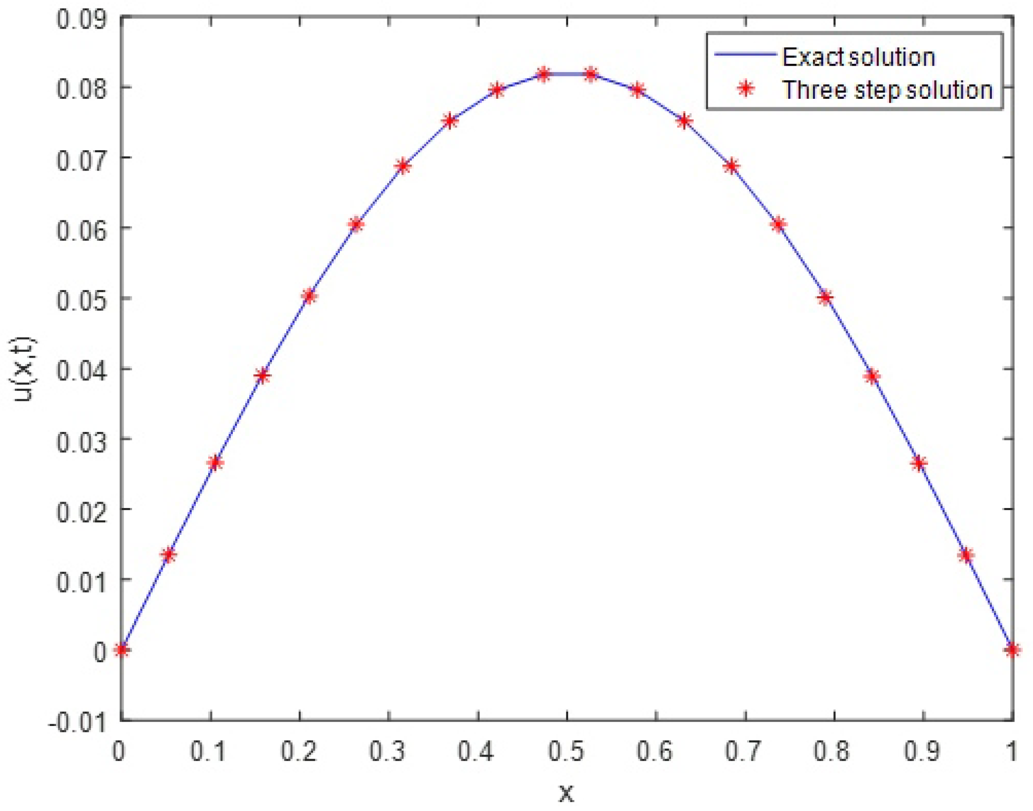
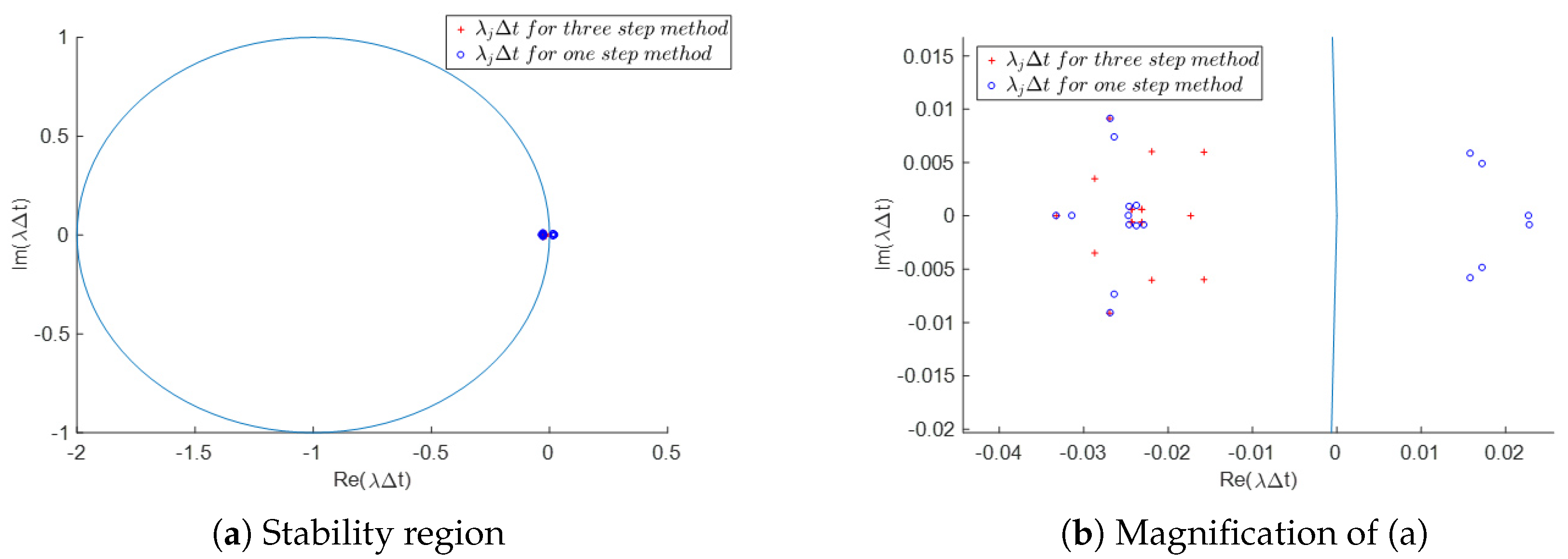
The exact and approximate solutions for the three-step wavelet collocation method are shown in Figure 3. The stability region for both three-step and one-step methods by choosing $M=8,k=1$ and $\Delta t=0.006$ is shown in Figure 4. As can be seen from this figure, there are some eigenvalues in the system of the one-step collocation method with $Re({\lambda }_j\Delta t)\notin [-2,0]$. Therefore, this method is not stable for $\Delta t=0.006$. In general, for $k=1$, the one-step collocation method shows a stable and accurate result if $\Delta t⩽0.001$, while the three-step collocation method is stable for $\Delta t⩽0.006$.

Example 3.

For the last example, consider Equation (6) with $\nu =1/{\pi }^2$, $\mu =0$, $f(x,t)=sin(\pi x)$, $g(x)=sin(\pi x)+cos(\pi x)$, $h_0(t)=e^{-t}$ and $h_1(t)=-e^{-t}$. The exact solution of this problem is $u_{exact}(x,t)=sin(\pi x)+e^{-t}cos(\pi x)$ [3].

Table 4. The $L_{\infty }$ error of Example 3 in $M=8$.

k	$\mathbf{\Delta }\mathit{t}$	Method in [17]	One-Step Method	Three-Step Method
1	$0.001$	$5.4341\times {10}^{-3}$	$3.7505\times {10}^{-4}$	$3.7552\times {10}^{-4}$
1	$0.006$	$6.3181\times {10}^{-3}$	unstable	$3.6961\times {10}^{-4}$
2	$0.001$	$4.5033\times {10}^{-3}$	$1.7750\times {10}^{-4}$	$1.6859\times {10}^{-4}$
2	$0.0016$	$4.2377\times {10}^{-3}$	unstable	$1.6772\times {10}^{-4}$

shows the maximum error for some different values using the one-step and three-step wavelet collocation methods. It is clear from this table that the one-step wavelet collocation method is unstable, while the three-step wavelet collocation method has a more precise response.

Figure 5 shows the three-step approximate solution and the exact solution. The stability region for both three-step and one-step methods by choosing $M=8,k=1$ and $\Delta t=0.006$ is shown in Figure 6.

6. Conclusions

In this paper, we proposed a new numerical method for a linear time-dependent partial differential equation. We called this method the three-step wavelet collocation method. In this method, time discretization was performed prior to the spatial discretization. These steps are equivalent to the third-order Taylor expansion; therefore, this method is third-order accurate in time. For spatial discretization, Legendre wavelets were used, which resulted in good spatial accuracy and spectral resolution. A comparison between the proposed method and other methods was presented. The theoretical aspect of absolute stability was discussed. This stability is based on ${\lambda }_j\Delta t$, where $\left\{{\lambda }_j\right\}$ are the eigenvalues of the corresponding system. Numerical performance shows that the three-step method leads to an effective time-accurate scheme with an improved stability property.

The proposed method can be easily implemented for other cases of time-dependent partial differential equations. For example, extending our results with Legendre wavelets in solving nonlinear partial differential equations or fractional equations is worthwhile for future contribution.

References

- Nouria, K.; Siavashani, N.B. Application of Shannon wavelet for solving boundary value problems of fractional differential equations. Wavelet Linear Algebra 2014, 1, 33–42. [Google Scholar]
- Kumar, B.V.R.; Mehra, M. A three-step wavelet Galerkin method for parabolic and hyperbolic partial differential equations. Int. J. Comput. Math. 2006, 83, 143–157. [Google Scholar] [CrossRef]
- Iqbal, M.A.; Ali, A.; Din, S.T.M. Chebyshev wavelets method for heat equations. Int. J. Mod. Appl. Phys. 2014, 4, 21–30. [Google Scholar]
- Zhou, F.; Xu, X. Numerical solution of the convection diffusion equations by the second kind Chebyshev wavelets. Appl. Math. Comput. 2014, 247, 353–367. [Google Scholar] [CrossRef]
- Mohammadi, F.; Hosseini, M.M. A new Legendre wavelet operational matrix of derivative and its applications in solving the singular ordinary differential equations. J. Frankl. Inst. 2011, 348, 1787–1796. [Google Scholar] [CrossRef]
- Maleknejad, K.; Sohrabi, S. Numerical solution of Fredholm integral equations of the first kind by using Legendre wavelets. J. Appl. Math. Comput. 2007, 186, 836–843. [Google Scholar] [CrossRef]
- Sahu, P.K.; Ray, S.S. Legendre wavelets operational method for the numerical solutions of nonlinear Volterra integro-differential equations system. Appl. Math. Comput. 2015, 256, 715–723. [Google Scholar] [CrossRef]
- Chena, Y.M.; Weia, Y.Q.; Liub, D.Y.; Yu, H. Numerical solution for a class of nonlinear variable order fractional differential equations with Legendre wavelets. Appl. Math. Lett. 2015, 43, 83–88. [Google Scholar] [CrossRef]
- Heydari, M.H.; Maalek Ghaini, F.M.; Hooshmandasl, M.R. Legendre wavelets method for numerical solution of time-fractional heat equation. Wavelet Linear Algebra 2014, 1, 15–24. [Google Scholar]
- Islam, S.U.; Aziz, I.; Al-Fhaid, A.S.; Shah, A. A numerical assessment of parabolic partial differential equations using Haar and Legendre wavelets. Appl. Math. Model. 2013, 37, 9455–9481. [Google Scholar] [CrossRef]
- Yin, F.; Tian, T.; Song, J.; Zhu, M. Spectral methods using Legendre wavelets for nonlinear Klein\Sine-Gordon equations. J. Comput. Appl. Math. 2015, 275, 321–324. [Google Scholar] [CrossRef]
- Luo, W.H.; Huang, T.Z.; Gu, X.M.; Liu, Y. Barycentric rational collocation methods for a class of nonlinear parabolic partial differential equations. Appl. Math. Lett. 2017, 68, 13–19. [Google Scholar] [CrossRef]
- Luo, W.H.; Huang, T.Z.; Wu, G.C.; Gu, X.M. Quadratic spline collocation method for the time fractional subdiffusion equation. Appl. Math. Comput. 2016, 276, 252–265. [Google Scholar] [CrossRef]
- Jiang, C.B.; Kawahara, M. A three-step finite element method for unstesdy incompressible flows. Comput. Mech. 1993, 11, 355–370. [Google Scholar] [CrossRef]
- Kashiyama, K.; Ito, H.; Behr, M.; Tezduyar, T. Three-step explicit finite element computation of shallow water flows on a massively parallel. Int. J. Numer. Meth. Fluids 1995, 21, 885–900. [Google Scholar] [CrossRef]
- Quartapelle, L. Numerical Solution of the Incompressible Navier-Stokes Equations; Springer Basel AG: Basel, Switzerland, 1993. [Google Scholar]
- Kumar, B.V.R.; Sangwan, V.; Murthy, S.V.S.S.N.V.G.K.; Nigam, M. A numerical study of singularly perturbed generalized Burgers-Huxley equation using three-step Taylor-Galerkin method. Comput. Math. Appl. 2011, 62, 776–786. [Google Scholar] [CrossRef]
- Ford, W. Numerical Linear Algebra with Applications Using MATLAB; Elsevier: Waltham, MA, USA, 2015. [Google Scholar]
- Toledo, S. Locality of reference in LU decomposition with partial pivoting. SIAM J. Matrix. Anal. Appl. 1997, 18, 1065–1081. [Google Scholar] [CrossRef]
- Canuto, C.; Quarteroni, A.; Hussaini, M.Y.; Zang, T.A. Spectral Methods in Fluid Dynamics; Springer: Berlin, Germany, 1988. [Google Scholar]
- Quarteroni, A.; Saleri, F. Scientific Computing with MATLAB and Octave; Springer: Berlin/Heidelberg, Germany, 2006. [Google Scholar]
- Kumar, B.V.R.; Mehra, M. A wavelet-taylor galerkin method for parabolic and hyperbolic partial differential equations. Int. J. Comput. Meth. 2005, 2, 75–97. [Google Scholar] [CrossRef]
- Lambert, J.D. Numerical Methods For Ordinary Differential Systems; John Wiley & Sons Ltd.: Hoboken, NJ, USA, 1991. [Google Scholar]
Figure 1.
The exact and approximate solutions of Example 1 in the case and .
Figure 2.
Stability region of Example 1 with the position of for , and . (b) is obtained from the magnification of (a).
Figure 3.
The exact and approximate solutions of Example 2 in the case and .
Figure 4.
Stability region of Example 2 with the position of for , and . (b) is obtained from the magnification of (a).
Figure 5.
The exact solution of Example 3 in the case and .
Figure 6.
Stability region of Example 3 with the position of for , and . (b) is obtained from the magnification of (a).