Abstract
Starting from the 2001 Thomas Friedrich’s work on , we review some interactions between and geometries related to octonions. Several topics are discussed in this respect: explicit descriptions of the canonical 8-form and its analogies with quaternionic geometry as well as the role of both in the classical problems of vector fields on spheres and in the geometry of the octonionic Hopf fibration. Next, we deal with locally conformally parallel manifolds in the framework of intrinsic torsion. Finally, we discuss applications of Clifford systems and Clifford structures to Cayley–Rosenfeld planes and to three series of Grassmannians.
Keywords:
Spin(9); octonions; vector fields on spheres; Hopf fibration; locally conformally parallel; Clifford structure; Clifford system; symmetric spaces MSC:
Primary 53C26; 53C27; 53C35; 57R25
1. Introduction
One of the oldest evidences of interest for the group in geometry goes back to the 1943 Annals of Mathematics paper by D. Montgomery and H. Samelson [1], which classifies compact Lie groups that act transitively and effectively on spheres, and gives the following list:
In particular, acts transitively on the sphere through its Spin representation, and the stabilizer of the action is a subgroup .
In the following decade, the above groups, with the only exception of , appeared in the celebrated M. Berger theorem [2] as the list of the possible holonomy groups of irreducible, simply connected, and non symmetric Riemannian manifolds. Next, in the decade after that, D. Alekseevsky [3] proved that is the Riemannian holonomy of only symmetric spaces, namely of the Cayley projective plane and its non-compact dual. Accordingly, started to be omitted in the Berger theorem statement. Much later, a geometric proof of Berger theorem was given by C. Olmos [4], using submanifold geometry of orbits and still referring to possible transitive actions on spheres.
Moreover, in the last decades of the twentieth century, compact examples have been shown to exist for almost all classes of Riemannian manifolds related to the other holonomy groups in the Berger list. References for this are the books by S. Salamon and D. Joyce [5,6,7]. For these reasons, around the year 2000, the best known feature of seemed to be that it was a group that had been removed from an interesting list.
Coming into the new millennium, since its very beginning, new interest in dealing with different aspects of octonionic geometry appeared, and new features of structures and weakened holonomies related to were pointed out. Among the references, there is, notably, the J. Baez extensive Bulletin AMS paper on octonions [8] as well as the not less extensive discussions on his webpage [9]. Next, and from a more specific point of view, there is the Thomas Friedrich paper on “weak -structures” [10], which proposes a way of dealing with a structure, and this was later recognized by A. Moroianu and U. Semmelmann [11] to fit in the broader context of Clifford structures. Also, the M. Atiyah and J. Berndt paper in Surveys in Differential Geometry [12] shows interesting connections with classical algebraic geometry. Coming to very recent contributions, it is worth mentioning the work by N. Hitchin [13] based on a talk for R. Penrose’s 80th birthday, which deals with in relation to further groups of interest in octonionic geometry.
The aim of the present article is to give a survey of our recent work on and octonionic geometry, in part also with L. Ornea and V. Vuletescu, and mostly contained in the references [14,15,16,17,18,19,20].
Our initial motivation was to give a construction, as simple as possible, of the canonical octonionic 8-form that had been defined independently through different integrals by M. Berger [21] and by R. Brown and A. Gray [22]. Our construction of uses the already mentioned definition of a -structure proposed by Thomas Friedrich and has a strong analogy with the construction of a -structure in dimension 8 (see Section 3 as well as [15]). By developing our construction of , we realized that some features of the sphere can be conveniently described through the same approach that we used. The fact that is the lowest dimensional sphere that admits more than seven global linearly independent tangent vector fields is certainly related to the Friedrich point of view. Namely, by developing a convenient linear algebra, we were able to prove that the full system of maximal linearly independent vector fields on any sphere can be written in terms of the unit imaginary elements in and the complex structures that Friedrich associates with (see Section 5 and [16]). Another feature of is, of course, that it represents the total space of the octonionic Hopf fibration, whose group of symmetries is . Here, the Friedrich approach to allows to recognize both the non-existence of nowhere zero vertical vector fields and some simple properties of locally conformally parallel -structures (here, see Theorem 4, Section 7, and Ref. [14]). We then discuss the broader contexts of Clifford structures and Clifford systems, that allow us to deal with the complex Cayley projective plane, whose geometry and topology can be studied by referring to its projective algebraic model, known as the fourth Severi variety. With similar methods, one can also study the structure and properties of the remaining two Cayley–Rosenfeld projective planes (for all of this, see Section 8, Section 9 and Section 10, and [17,18]). Finally, Clifford structures and Clifford systems can be studied in relation with the exceptional symmetrical spaces of compact type as well as with some real, complex, and quaternionic Grassmannians that carry a geometry very much related to octonions (see Section 11 and Section 12, and [19,20]).
During the years of our work, we convinced ourselves that influences not only 16-dimensional Riemannian geometry, but also aspects related to octonions of some lower dimensional and higher dimensional geometry. It is, in fact, our hope that the reader of this survey can share the feeling of the beauty of , that seems to have some role in geometry, besides being a group that had been removed from an interesting list.
2. Preliminaries, Hopf Fibrations, and Friedrich’s Work
The multiplication involved in the algebra () of octonions can be defined from the one in quaternions () by the Cayley–Dickson process: if , , then
where are the conjugates of . As for quaternions, the conjugation is related to the non-commutativity: The associator
vanishes whenever two among are equal or conjugate. For a survey on octonions and their applications in geometry, topology, and mathematical physics, the excellent article [8] by J. Baez is a basic reference.
The 16-dimensional real vector space decomposes into its octonionic lines,
that intersect each other only at the origin . Here, parametrizes the set of octonionic lines (l), whose volume elements () allow the following canonical 8-form on to be defined:
where denotes the orthogonal projection .
The definition of through this integral was given by M. Berger [21], and here we chose the proportionality factor in such a way to make integers and with no common factors the coefficients of as exterior 8-form in . The notation is motivated by the following:
Proposition 1.
[23] The subgroup of preserving is the image of under its spin representation into .
Thus, , so that 16-dimensional oriented Riemannian manifolds are the natural setting for -structures. The following definition was proposed by Th. Friedrich, [10].
Definition 1.
Let be a 16-dimensional oriented Riemannian manifold. A structure on M is the datum of any of the following equivalent alternatives.
- 1.
- A rank 9 subbundle, , locally spanned by endomorphisms withwhere denotes the adjoint of .
- 2.
- A reduction, , of the principal bundle, , of orthonormal frames from to .
In particular, the existence of a structure depends only on the conformal class of the metric g on M.
We now describe the vector bundle when M is the model space (). Here, can be chosen as generators of the Clifford algebra (), the endomorphisms’s algebra of its 16-dimensional real representation, . Accordingly, unit vectors () can be viewed via the Clifford multiplication as symmetric endomorphisms: .
The explicit way to describe this action is by (, , ), acting on pairs :
where denotes the right multiplications by , respectively (cf. [24] (p. 288)).
A basis of the standard structure on can be written by looking at action (4) and at the following nine vectors:
where , , and , and their products are ruled by (1). This gives the following symmetric endomorphisms:
where are the right multiplications by the 7 unit octonions, . Their spanned subspace
is such that the following proposition applies.
Proposition 2.
[23] The subgroup of preserving is
The projection associated with decomposition into the octonionic lines , is a non-compact version of the octonionic Hopf fibration:
that is the unique surviving possibility when passing from quaternions to octonions from the series of quaternionic Hopf fibrations:
Recall that the latter enter into Figure 1 that encodes prototypes of several structures of interest in quaternionic geometry.
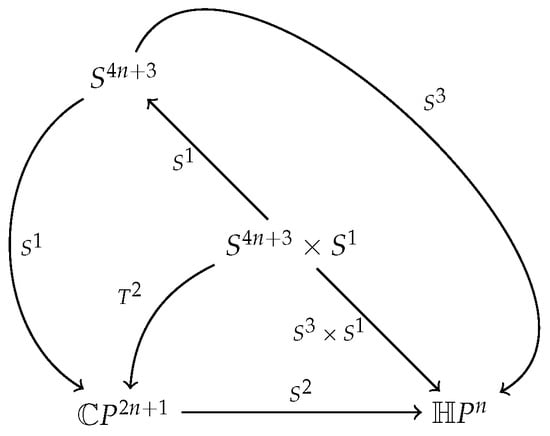
Figure 1.
The prototype of foliations related to locally conformally hyperkähler manifolds.
At the center of the diagram, there is the locally conformally hyperkähler Hopf manifold . All the other manifolds are leaf spaces of foliations on them, such as the 3-Sasakian sphere , the positive Kähler-Einstein twistor space , and the positive quaternion Kähler . Most of the foliations carry similar structures on their leaves, for example, one has locally conformally hyperkähler Hopf surfaces of . This prototype diagram is only an example, since, when a compact locally hyperkähler manifold has compact leaves on the four canonically defined vertical foliations, our diagram still makes sense, albeit in the broader orbifold category (cf. [25]).
When , there are also the octonionic Hopf fibrations, as in Figure 2:
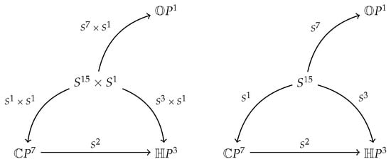
Figure 2.
In the octonionic case, an additional fibration appears.
These have no arrow connecting with and , since the complex and quaternionic Hopf fibrations are not subfibrations of the octonionic one (cf. [26] as well as Theorem 4 in the following Section 6).
Coming back to , as the title of Th. Friedrich’s article [10] suggests, there is a scheme for “weak structures” to include some possibilities besides the very restrictive holonomy condition. Although the original A. Gray proposal [27] to look at “weak holonomies” was much later shown by B. Alexandrov [28] not to produce new geometries for the series of groups quoted in the Introduction, one can refer to the symmetries of relevant tensors to understand the possibilities for any G-structure. We briefly recall a unified scheme that one can refer to, following the presentation of Ref. [29].
By definition, a G-structure on an oriented Riemannian manifold () is a reduction () of the orthonormal frame bundle to the subgroup . The Levi Civita connection (Z), thought of as a 1-form on with values in the Lie algebra , restricts to a connection on , decomposing with respect to the Lie algebra splitting , as
Here, is a connection in the principal G-bundle , and is a 1-form on with values in the associated bundle , called the intrinsic torsion of the G-structure. Of course, the condition is equivalent to the inclusion for the Riemannian holonomy, and G-structures with are called non-integrable.
This scheme can be used, in particular, when G is the stabilizer of some tensor in , so that the G-structure on M defines a global tensor , and here, can be conveniently thought of as a section of the vector bundle:
Accordingly, the action of G splits into irreducible G-components: .
A prototype of such decompositions occurs when and yields the four irreducible components of the so-called Gray–Hervella classification when [30]. It is a fact from the representation theory that there are several further interesting cases that yield four irreducible components. This occurs when , as computed in Refs. [31], ([32] (p. 115)) and [10], respectively:
For the mentioned four situations, the last component, , is the “vectorial type” one, and gives rise to a 1-form on the manifold. A general theory of G-structures in this last class, , of typically locally conformally parallel G-structures, was developed in Ref. [33]. In Section 7, we revisit in the case, following Ref. [10] as well as our previous work [14].
3. The Canonical 8-Form
The space of 2-forms in decomposes under as
(cf. [10] (p. 146)), where and is an orthogonal complement in . Explicit bases of both subspaces can be written by looking at the nine generators (5) of the vector space that defines the structure. Namely, one has the compositions
for as a basis of and the compositions for as a basis of .
The Kähler 2-forms () of the complex structures , obtained by denoting the coordinates in by are
where denotes the of what appears before it, for instance
Next,
and a computation gives the following proposition.
Proposition 3.
In particular, , and the -invariant 8-form has to be proportional to . The proportionality factor, computed by looking at any of the terms of and turns out to be 360.
This can be rephrased in the context of structures on Riemannian manifolds and gives the following two (essentially equivalent) algebraic expressions for the the 8-form, :
Theorem 1.
[34] The 8-form, , associated with the -structure and defined by the integral (2) coincides, up to a constant, with the global form
Theorem 2.
[15] The 8-form, , associated with the -structure coincides, up to a constant, with the coefficient
in the characteristic polynomial
where is any skew-symmetric matrix of local associated Kähler 2-forms (M). The proportionality factor is given by
These two expressions of have been shown to be proportional according to the following algebraic relation.
Proposition 4.
[35] Let be the polynomial ring in the 36 variables (), and let x be the skew-symmetric matrix whose upper diagonal entries are . Among the homogeneous polynomials
the following relation holds: . Thus, since ,
Corollary 1.
The Kähler forms of the -structure of allow the integral (2) to be computed as
When is the holonomy group of the Riemannian manifold (), the Levi–Civita connection (∇) preserves the vector bundle, and the local sections of induce the Kähler forms on M as the local curvature forms.
Corollary 2.
Let be a compact Riemannian manifold with holonomy , i.e., is either isometric to the Cayley projective plane () or to any compact quotient of the Cayley hyperbolic plane (). Then, its Pontrjagin classes are given by
Proof.
The Pontrjagin classes of the vector bundle are given by
For a compact M with a -structure, the following relations hold ([10] (p. 138)):
Thus, gives , so that , , and . ☐
The Pontrjagin classes of are known to be and , where u is the canonical generator of , and Corollary 2 gives the representative forms:
Remark 1.
Very recently, an alternative way of writing the 8-form in was proposed by J. Kotrbatý [36]. This is in terms of the differentials of the octonionic coordinates . If
consider, formally, the “octonionic 4-forms”
Then, by defining their conjugates through
for Kotrbatý shows that the real 8-form
gives the proportionality relation and recovers the table of 702 non-zero monomials of in from this.
4. The Analogy with
In the previous Section we saw that the matrices are the starting point for the construction of the canonical 8-form . Of course, are the octonionic analogues of the classical Pauli matrices
which are defined with just the unit imaginary , belonging to U(2). Their compositions (), for act on as multiplications on the right by unit quaternions: .
Similarly, the quaternionic analogues of the Pauli matrices are the real matrices:
where are the multiplication on the right on by .
The ten compositions of these latter matrices are a basis of the term in the decomposition
where . Their Kähler forms read
If , it follows that
where ⋆ denotes the Hodge star of what appears before, and
is the left quaternionic 4-form on .
On the other hand, the matrices which commute with each of the involutions are the ones satisfying and . Thus, the subgroup preserving each of the is the diagonal . Thus, the subgroup of preserving the vector bundle consists of matrices (B) satisfying
with and bases of related by a matrix. This group is thus recognized to be , and the following proposition applies.
Proposition 5.
Let be an 8-dimensional oriented Riemannian manifold, and let be a vector subbundle of , locally spanned by self dual anti-commuting involutions () and related, on open sets covering M, by functions giving matrices. Then, the datum of such an is equivalent to an (left) almost quaternion Hermitian structure on M, i.e., to a -structure on M.
In the above discussions, we looked at the standard U(2) and -structures on and , through the decompositions of the 2-forms
and the orthonormal frames in the and components, respectively. The last components, and , describe all of the similar structures on the linear spaces and . Thus, such decompositions give rise to the and spaces—the spaces of all possible structures in the two cases.
To summarize (cf, [37]),
Corollary 3.
The actions , when (and, in any case, and ) generate the groups U(2), , of symmetries of the Hopf fibrations
The corresponding G-structures on the Riemannian manifolds , , can be described through vector subbundles of ranks , respectively. Any such E is locally generated by the self-dual involutions satisfying for and related, on open neighborhoods covering M, by functions that give matrices in , , and .
5. Vector Fields on Spheres
An application of structures is the possibility of writing a maximal orthonormal system of tangent vector fields on spheres of any dimension. Here, we outline this construction only on some “low-dimensional” cases (in fact. up to the sphere), referring, for the general case, to the linear algebra formalism developed in Ref. [16].
Recall that the identifications , and allow to act on the normal vector field of the unit sphere by the imaginary units of , giving 1, 3, and 7 tangent orthonormal vector fields on , , and . These are, in fact, a maximal system of linearly independent vector fields on , provided the (even) dimension (m) of the ambient space is not divisible by 16. The maximal number () of linearly independent vector fields on any is well-known to be expressed as
where is the Hurwitz–Radon number, referring to the decomposition
(cf. Ref. [16] for further information and references on this classical subject).
Table 1 lists some of the lowest dimensional spheres that admit a maximal number of linearly independent vector fields.

Table 1.
Some spheres with more than seven vector fields.
The first of them is , which is acted on by . To write the eight vector fields on , it is convenient to look at the involutions and at the eight complex structures () on :
Denote by
the (outward) unit normal vector field of . Then, the following proposition applies.
Proposition 6.
The vector fields
are tangent to and orthonormal.
Indeed, by fixing any , and considering the 8 complex structures with , the eight vector fields () are still tangential to and orthonormal.
Although it is well-known that , and are the only normed algebras over , to move to a higher dimension, it is convenient to consider the algebra of sedenions, obtained from through the Cayley–Dickson process. By denoting the canonical basis of over by , one can write a multiplication table (cf. Ref. [16]). An example of divisors of the zero in is given by .
The following remark helps in higher dimensions. Consider the sphere, and decompose m as , where . First, observe that a vector field (B) that is tangential to the sphere induces a vector field
that is tangential to the sphere. Thus, assume in what follows that , i.e., . Whenever we extend a vector field in this way, we call the vector field given by (17) the diagonal extension of B.
If , that is, if m is not divisible by 16, the vector fields on are given by the complex, quaternionic, or octonionic multiplication for , or 3 respectively, so that the contribution occurs when , that is, , and we can denote the coordinates in by , where each , for , belongs to the sedenions (), and can thus be identified with a pair () of octonions.
The unit (outward) normal vector field (N) of can be denoted by using the sedenions:
Therefore, we can think of N as an element of .
Whenever , or 8, denoted by , the following automorphism of applies.
We refer to as a conjugation, due to its similarity to that in *-algebras.
Moreover, it is convenient to use the following formal notations:
which allow us to define left multiplications () in the sedenionic spaces , , and (like in , , and ), as follows.
If , the left multiplication is
whereas, if , we define
and finally, if , we define
Note that, in all three cases, , and 8, and the vector fields are tangential to , , and , respectively.
We can now write the maximal systems of vector fields on , , and , as follows.
Case
For , whose maximal number of tangent vector fields is nine, we obtain eight vector fields by writing the unit normal vector field as , where , and repeating Formula (16) for each pair ():
A ninth orthonormal vector field, completing the maximal system, is found by the formal left multiplication (22) and the automorphism (18):
Case
The sphere has a maximal number of 11 orthonormal vector fields. The normal vector field is, in this case, given by , and eight vector fields arise as , for . Three other vector fields are again given by the formal left multiplications (23) and the automorphism in (18):
Case
The sphere has a maximal number of 15 orthonormal vector fields. Eight of them are still given by for , whereas the formal left multiplications given in (24) yield the seven tangent vector fields (), for .
The sphere
To write a system of 16 orthonormal vector fields on , decompose
into sixteen components. The unit outward normal vector field is
where are sedenions.
The matrices in which give the complex structures act on N not only separately on each of the 16-dimensional components of (28), but also formally on the (column) 16-ples of sedenions . Based on which of the two actions of the same matrices are considered in , we use the notations
in both cases being all complex structures on . The following 16 vector fields are obtained:
where is defined in Formula (18). The level 1 vector fields and level 2 vector fields are the ones given by (29) and (30), respectively. Then, the following proposition applies.
Proposition 7.
Proof.
Denote sedenions as pairs of octonions. The unit normal vector field is
and one gets the following tangent vectors that can be easily checked to be orthonormal:
Moreover, one obtains eight further vector fields which can be similarly verified to be orthonormal.
To see that each vector is orthogonal to each , for , look at the matrix representations of and write the octonionic coordinates as , . Then, the scalar product can be computed with Formula (1) to obtain the product of the octonions. For example, recall from Formula (32) that
so that the computation of gives rise to pairs of terms like in
To conclude, observe that the real part (ℜ) of the sums of each of the corresponding underlined terms is zero. This is due to the identity (), that holds for all . ☐
More generally, the following proposition applies.
Proposition 8.
Fix any β, , consider the eight complex structures , with , defined on by acting with the corresponding matrices on the listed 16-dimensional components, that is, the diagonal extension of . Also, consider the further eight complex structures for , defined by the same matrices that now act on the column matrix of sedenions (). Then,
is a maximal system of 16 orthonormal tangent vector fields on .
The dimension, that is, the sphere, is the lowest dimensional case where the last ingredient of our construction enters. To define the additional vector field here, we need to extend the formal left multiplication defined by Formula (22). Consider the decomposition
and denote the elements in by . Using the notation
a formal left multiplication ( in ) can be defined with Formula (22). It can then be expected that is orthogonal to , but this is not the case. In fact, appears to be orthogonal to the first eight vector fields but not to the second ones.
To make things work, we need to extend not only , but also the D conjugation. To this aim, the elements are split into where , and the conjugation is defined on using Formula (18):
The additional vector field is then , and the following theorem applies.
Theorem 3.
A maximal orthonormal system of tangent vector fields on is given by the following vector fields:
6. Back to the Octonionic Hopf Fibration
As we saw in the previous Section, is the lowest dimensional sphere with more than seven linearly independent vector fields. There are further features that distinguish among spheres. For example, is the only sphere that admits three homogeneous Einstein metrics, and it is the only sphere that appears as a regular orbit in three cohomogeneity actions on projective spaces, namely, of , , and on , , and , respectively (see Refs. [38,39]). All of these features can be traced back to the transitive action of on the octonionic Hopf fibration . The following theorem applies.
Theorem 4.
Any global vector field on which is tangent to the fibers of the octonionic Hopf fibration has at least one zero.
Proof.
For any , we already denoted by
the (outward) unit normal vector field of in . After identifying the tangent spaces with , it can be noted that the involutions define the following sections of :
Their span,
is, at any point, a nine-plane in that is not tangential to the sphere. Observe that the nine-plane is invariant under . This is certainly the case for the single vector field N, since . On the other hand, the endomorphisms rotate under the action inside their vector bundle.
Next, note that contains N:
where the coefficients are computed from (37) in terms of the inner products of vectors,
and of the right translations, , as follows:
In particular, at points with , that is, on the octonionic line , the vector fields are orthogonal to the unit sphere. The latter is the fiber of the Hopf fibration over the north pole (), and the mentioned orthogonality of this fiber () is immediate from (37) for
Also, at these points, we have , so is orthogonal to the fiber as well. Now, the invariance of the octonionic Hopf fibration under shows that all its fibers are characterized as being orthogonal to the vector fields in .
Now, assume that X is a vertical vector field of . From the previous characterization, we have the following orthogonality relations in :
and it follows that . However, from the definition of a structure, it can be observed that if , then . Thus, if X is a nowhere zero vertical vector field, we obtain, in this way, nine pairwise orthogonal vector fields () that are all tangent to . However, is known to admit, at most, eight linearly independent vector fields. Thus, X cannot be vertical and nowhere zero. ☐
One gets, as a consequence, the following alternative proof of a result, established in Ref. [26].
Corollary 4.
The octonionic Hopf fibration does not admit any subfibration.
Proof.
In fact, any subfibration would give rise to a real line sub-bundle () of the vertical sub-bundle of . This line bundle (L) is necessarily trivial, due to the vanishing of its first Stiefel–Whitney class, . It follows that L would admit a nowhere zero section and thus, a global, vertical, nowhere zero vector field. ☐
7. Locally Conformally Parallel Manifolds
Let . Recall that a locally conformally parallel G-structure on a manifold is the datum of a Riemannian metric (g) on a covering of and for each , a metric defined on which has holonomy contained in G such that the restriction of g to each is conformal to :
for some smooth map () defined on
Some of the possible cases here are
- G = U(n), where we have the locally conformally Kähler metrics;
- , yielding the locally conformally quaternion Kähler metrics;
- which is the case we are dealing with.
In any of the cases above, for each overlapping , the functions differ by a constant:
This implies that on , hence defining a global, closed 1-form that is usually denoted by and called the Lee form. Its metric dual with respect to g is denoted by N as
and is called the Lee vector field.
The G = U(n) case of locally conformally Kähler metrics has been extensively studied in the last decades (see, for instance, Ref. [40]).
When G is chosen to be or , there are close relations to 3-Sasakian geometry (see Ref. [25] or the surveys [41,42]). Finally, locally conformally parallel and structures were studied in Ref. [43], and they relate to nearly parallel and geometries, respectively.
As mentioned in the Introduction, the holonomy of is only possible on manifolds that are either flat or locally isometric to or to the hyperbolic Cayley plane . Weakened holonomy conditions give rise to several classes of structures (cf. Ref. [10] and Section 2). One of these classes is that of vectorial type structures (see Refs. [33] and [10] (p. 148)). According to the following Definition and the following Remark, this class fits into the locally conformally parallel scheme.
Definition 2.
[33] A structure is of the vectorial type if Γ lives in .
Remark 2.
In Refs. [10,33], the class of locally conformally parallel structures has been identified and studied under the name structures of vectorial type. Now, we outline now a proof that, for structures, the vectorial type is equivalent to the locally conformally parallel type. As already mentioned in Section 2, the splitting of the Levi–Civita connection, viewed as a connection in the principal bundle of orthonormal frames on M is
where is the connection of -frames in the induced bundle, and Γ is its orthogonal complement. Thus, Γ is a 1-form with values in the orthogonal complement in the splitting of Lie algebras , and under the identification (cf. the beginning of Section 3), Γ can be seen as a 1-form with values in . Under the action of , the space decomposes as a direct sum of four irreducible components:
and looking at all the possible direct sums, this yields 16 types of structure. Component identifies with , and thus, with the component in Formula (7).
Now, let be a Riemannian manifold endowed with a structure of the vectorial type. Let be as above, and let be its -invariant 8-form. Now, implies that the holonomy of M is contained in (cf. Ref. [10] (p. 21)).
From Ref. [33] (p. 5), we know that the following relations hold:
Let be the Riemannian universal cover of , and let , be the lifts of and respectively. Then, relations (38) also hold for and . Since is simply connected, for some . Then, by defining and , we have , that is, the -factor of is zero. Hence, has holonomy contained in , and on the other hand, it is locally conformal to g. Thus, M can be covered by open subsets on which the metric is conformal to a metric with holonomy in .
The conformal flatness of metrics with holonomy has the following consequences (cf. Ref. [14] for the proofs).
Theorem 5.
Let be a compact manifold that is equipped with a locally, non globally, conformally parallel metric g. Then,
- 1.
- The Riemannian universal covering of M is conformally equivalent to the euclidean , the Riemannian cone over , and M is locally isometric to up to its homotheties.
- 2.
- M is equipped with a canonical 8-dimensional foliation.
- 3.
- If all the leaves of are compact, then M fibers over the orbifold are finitely covered by , and all fibers are finitely covered by .
Theorem 6.
Let be a compact Riemannian manifold. Then, is locally, non globally, conformally parallel if and only if the following three properties are satisfied:
- 1.
- M is the total space of a fiber bundle where π is a Riemannian submersion over a circle of radius r.
- 2.
- The fibers of π are spherical space forms (), where K is a finite subgroup of .
- 3.
- The structure group of π is contained in the normalizer of K in .
8. Clifford Systems and Clifford Structures
The self dual anti-commuting involutions that define the standard -structure on are an example of a Clifford system. The definition, formalized in 1981 by D. Ferus, H. Karcher, and H. F. Münzner, in their study of isometric hypersurfaces of spheres [44], is the following.
Definition 3.
A Clifford system on the Euclidean vector space is the datum
of a -ple of symmetric endomorphisms such that
A Clifford system on is said to be irreducible if is not a direct sum of two positive dimensional subspaces that are invariant under all the .
From the representation theory of Clifford algebras, it is recognized (cf. Refs. [44] (p. 483) and [45] (p. 163)) that admits an irreducible Clifford system () if and only if , where is given as in the following Table 2.
Table 2.
Clifford systems.
Uniqueness can be discussed as follows. Given, on , two Clifford systems ( and ), they are said to be equivalent if exists such that for all . Then, for mod 4, there is a unique equivalence class of irreducible Clifford systems, and for mod 4, there are two, which are classified by the two possible values of the trace .
In Ref. [18], we outlined the following inductive construction for the irreducible Clifford systems on real Euclidean vector spaces (), taking, as starting the point, the basic Clifford systems () associated with structures given by U(1), U(2), , and . All the cases appearing in Table 2 and Table 3 make sense in the natural context of Riemannian manifolds. We get the following theorem (see Ref. [18] for details).
Table 3.
Clifford systems and G-structures on Riemannian manifolds ().
Theorem 7.
(Procedure to write new Clifford systems from old). Let be the last (or unique) Clifford system in . Then, the first (or unique) Clifford system,
in has, respectively, the following first and last endomorphisms:
where the blocks are . The remaining matrices are
Here, are the complex structures given by compositions in the Clifford system . When the complex structures () can be viewed as (possibly block-wise) right multiplications by some of the unit quaternions () or unit octonions (), and if the dimension permits it, further similarly defined endomorphisms () can be added by using some others among or .
The notion of an even Clifford structure, a kind of unifying notion proposed by A Moroianu and U. Semmelmann [11], is instead given by the following datum on a Riemannian manifold ().
Definition 4.
An even Clifford structure on is a real oriented Euclidean vector bundle , together with an algebra bundle morphism () which maps into skew-symmetric endomorphisms.
By definition, a Clifford system always gives rise to an even Clifford structure, but there are some even Clifford structures on manifolds that cannot be constructed, even locally, from Clifford systems. An example of this is given by a structure on any oriented 8-dimensional Riemannian manifold as a consequence of the following observations (cf. Ref. [15] for further details).
Proposition 9.
Let be a Clifford system in . The compositions for , and for are linearly independent complex structures on .
Proof.
It can be easily recognized that and are complex structures. On the other hand, for any , it can be observed that , and for , , so that the are orthonormal and symmetric. By a similar argument, and if or equals or . Also, for and , the is the composition of the skew-symmetric and the symmetric , and as such, its trace is necessarily zero. Similar arguments show that the for are orthonormal. ☐
Corollary 5.
The -structures on cannot be defined through Clifford system .
Proof.
For any choice of such a Clifford system, in , the complex structures for give rise to 35 linearly independent skew-symmetric endomorphisms, contradicting the decomposition of 2-forms in under :
☐
Nevertheless, the right multiplications by span the vector bundle, and this identifies structures among the even Clifford structures.
The following Sections present further examples of such essential Clifford structures, i.e., Clifford structures not coming from Clifford systems.
On Riemannian manifolds (), it is natural to consider the following class of even Clifford structures.
Definition 5.
The even Clifford structure on is said to be parallel if a metric connection () exists on E such that φ is connection preserving, i.e.,
for every tangent vector and section σ of , and where is the Levi–Civita connection.
Table 4 summarizes the non-flat, parallel, even Clifford structure, as classified in Ref. [11]. The non-compact duals of the appearing symmetric spaces have to be added. A good part of the listed manifolds appear in the following sections.
Table 4.
Parallel, non-flat, even Clifford structures (cf. Ref. [11]).
9. The Complex Cayley Projective Plane
This section deals with
the second, after the Cayley projective plane (), of the exceptional symmetric spaces appearing in Table 4.
A remarkable feature of , one of the two exceptional Hermitian symmetric spaces of compact type, is its model as a smooth projective algebraic variety of complex dimension 16 and degree 78, the so-called fourth Severi variety . This name was proposed by F. Zak [46], who classified the smooth projective algebraic varieties () in a that, in spite of their critical dimension (), are unable to fill through their chords.
On the other hand, admits a construction that is very similar to the one of the Cayley projective plane (). One can, in fact, look at the complex octonionic Hermitian matrices
which are acted on by with three orbits on . The closed one consists of Z matrices of rank one,
and, as such, can be thought as (virtual) “projectors on complex octonionic lines in ”; thus, they are points of the complex projective Cayley plane .
The projective algebraic geometry of was studied in detail in Ref. [47]. Similarly to Corollary 5, we have the following proposition.
Proposition 10.
The complex space does not admit any family of ten endomorphisms () that satisfies the properties of a Clifford system and is compatible with respect to the standard Hermitian scalar product g.
Proof.
The family would define (after multiplying each of them by i) a representation of the complex Clifford algebra (the order 32 complex matrix algebra) on the vector space. ☐
Note, however, that the Euclidean space admits the Clifford system (cf. Table 2). The parallel, even Clifford structure on can be defined through the following one, here described on the model space.
For this, observe that is generated as a Lie algebra by and , with spanned by
where
The rank 10 even Clifford structure on is then given by the vector bundle
and
We get the following theorem (cf. Proposition 3 and Theorem 4).
Theorem 8.
[17] Let be the even Clifford structure on . In accordance with the previous notations, the characteristic polynomials
of the matrix
of Kähler 2-forms of the give:
- (i)
- where ω is the Kähler 2-form of E III;
- (ii)
- is the primitive generator of the cohomology ring .
In analogy with the situation (Section 3), is called the canonical 8-form on .
Moreover, the following theorem applies.
Theorem 9.
Let ω be the Kähler form, and let be the previously defined 8-form on . Then:
- (i)
- The de Rham cohomology algebra is generated by (the classes of) and .
- (ii)
- By looking at as the fourth Severi variety (), the de Rham dual of the basis represented in by the forms is given by the pair of algebraic cycleswhere are maximal linear subspaces that belong to the two different families ruling a totally geodesic, non-singular, quadric contained in .
10. Cayley–Rosenfeld Planes
Besides the real and the complex Cayley projective planes and , there are two further exceptional symmetric spaces of compact type, that are usually referred to as the Cayley–Rosenfeld projective planes, namely, the “projective plane over the quaternionic octonions”:
and the “projective plane over the octonionic octonions”:
By referring to the inclusions , it can be observed that the projective geometry of these four projective planes, which is notably present on the first two steps, becomes weaker at the third and fourth Cayley–Rosenfeld projective planes (cf. Ref. [8]). However, the dimensions of these four exceptional symmetric spaces are coherent with this terminology. According to Table 4, these four spaces have the highest possible ranks for non-flat, parallel, even Clifford structures.
The following Table 5 summarizes the even Clifford structures on the four Cayley–Rosenfeld planes. Only the one on is given by a Clifford system; the other three are essential. Concerning the cohomology generators, the one in dimension 8 can also be constructed for and via the fourth coefficient () of the matrices () of Kähler 2-forms that are associated with the even Clifford structures that we are now listing.
Table 5.
Even Clifford structures on the Cayley–Rosenfeld projective planes.
Remark 3.
The matrices of the Kähler 2-forms that are associated with the even Clifford structures go through
and the last Lie algebra decomposes as
By recalling the identification
(cf. the observation after (8) as well as [18]), this identification takes back the even Clifford structure of the 128-dimensional Cayley–Rosenfeld plane () to the -structures that we started with.
11. Exceptional Symmetric Spaces
A good number of symmetric spaces that appear in Table 4 belong to the list of exceptional Riemannian symmetric spaces of compact type,
that are part of the E. Cartan classification. Among them, the two exceptional Hermitian symmetric spaces,
are Kähler and therefore, are equipped with a non-flat, parallel, even Clifford structure of rank . Next, the five Wolf spaces
which are examples of positive quaternion Kähler manifolds, carry a rank of in a non-flat, parallel, Clifford structure.
Thus, seven of the twelve exceptional, compact type, Riemannian symmetric spaces of are either Kähler or quaternion Kähler. Accordingly, one of their de Rham cohomology generators is represented by a Kähler or quaternion Kähler form, and any further cohomology generators can be viewed as primitive in the sense of the Lefschetz decomposition.
As seen in the previous sections, the four Cayley–Rosenfeld projective planes,
carry a similar structure with .
Thus, among the exceptional symmetric spaces of compact type, there are two spaces that admit two distinct even Clifford structures, namely, the Hermitian symmetric has even Clifford structures of rank 2 and of rank 10, and the quaternion Kähler has even Clifford structures of rank 3 and rank of 12. For simplicity, we call octonionic Kähler the parallel even Clifford structure defined by the vector bundles on the Cayley–Rosenfeld projective planes (). In conclusion, and with the exceptions of
nine of the twelve exceptional Riemannian symmetric spaces of compact type admit at least one parallel, even Clifford structure. Any of such structures gives rise to a canonical differential form: the Kähler 2-form for the complex Kähler one, the quaternion Kähler 4-form for the five Wolf space, and a canonical octonionic Kähler 8-form for the four Cayley–Rosenfeld projective planes. Their classes are always one of the cohomology generators, and Table 6 collects some informations on the exceptional symmetric spaces of compact type. For each of them, the real dimension, the existence of torsion in the integral cohomology, the Kähler or quaternion Kähler or octonionic Kähler (K/qK/oK) property, the Euler characteristic , and the Poincaré polynomial (up to mid dimension) are listed.
Table 6.
Exceptional, compact type, symmetric spaces.
Next, we have Table 7 which contains the primitive Poincaré polynomials
of the nine exceptional Riemannian symmetric spaces that admit an even parallel Clifford structure. Here, the meaning of “primitive” varies depending on the considered K/qK/oK structure. Thus, the Hermitian symmetric spaces, and , are simply polynomials with coefficients the primitive Betti numbers,
where is the Lefschetz operator which multiplies the cohomology classes with the complex Kähler form , and n is the complex dimension.
Table 7.
Primitive Poincaré polynomials, .
In the positive quaternion Kähler setting, the vanishing of odd Betti numbers and the injectivity of the Lefschetz operator , , now occur with being the quaternion 4-form and n being the quaternionic dimension. A remarkable aspect of the primitive Betti numbers
for positive quaternion Kähler manifolds is their coincidence with the ordinary Betti numbers of the associated Konishi bundle—the 3-Sasakian manifold fibering over it (cf. [48] (p. 56)).
Finally, on the four Cayley–Rosenfeld planes, the vanishing of odd Betti numbers and the injectivity of the map still occur, and are defined by multiplication with the octonionic 8-form , and with , where n is now the octonionic dimension.
12. Grassmannians
Table 4 contains the following three series of Grassmannians:
that carry an even Clifford structure of rank , respectively.
To define them, recall that the subgroup is generated by the following matrices:
where
(cf. Ref. [49]). For the orthonormal , matrices satisfy the properties
On the other hand, recall that
where W is the tautological vector bundle, and its orthogonal complement in the ambient linear space.
Finally, it is convenient to recall that the complex structure and the local compatible hypercomplex structures of the following complex Kähler and quaternion Kähler Grassmannians,
come visibly from their elements, which are, respectively, oriented 2-planes, oriented 4-planes, and complex 2-planes.
Look first at Grassmannians in the first of the three series (40), namely, at , referring, for simplicity, to the case of an even dimensional ambient space, , and thus insuring the spin property of the Grassmannian. From the local orthonormal bases and of sections respectively of W and of , one gets the following local basis of the tangent vectors of :
The listed 8-ples of sections can be written formally as octonions, i.e., for ,
and this can be ordered as a n-ple of pairs of octonions:
The even Clifford structure on can then be defined by looking at a rank 8 Euclidean vector bundle that satisfies the condition of being locally generated by anti-commuting orthogonal complex structures. Here, this is denoted by , in correspondence with the . The existence of such an E is insured by the holonomy structure of the Grassmannian, by its spin property, and by the given description of . Accordingly, if are local sections of E, we can look at them as octonions in the basis .
For any such orthonormal pair , look at as a section of , and define
by
i.e., by diagonally applying the matrix (41). When this is extended by the Clifford composition, this gives the Clifford morphism
Thus, the following theorem applies.
Theorem 10.
There is a rank 8 vector sub-bundle that is locally generated by the anti-commuting orthogonal complex structures , and E defines an even, non-flat, parallel Clifford structure of rank 8 on . The morphism
is given by the Clifford extension of the map,
which is defined by diagonally applying the matrix . Here, are local orthonormal sections of E; thus, unitary orthogonal octonions in the basis , so that acts diagonally on the m-ples of pairs of local tangent vectors,
that can be looked at as elements of .
A similar statement holds for the second series of Grassmannians in (40), assuming again an even dimensional ambient space, . Let and be the local orthonormal bases of W and , respectively. Define the following local tangent vector fields as local sections of :
Again, look at the above lines as
(), and order them as m-ples of pairs:
Now consider the vector sub-space , and note that the corresponding operators (, with ), act on the complex vector space (). Similarly to what was described for the real Grassmannians, there is a vector sub-bundle, , that is locally generated by the anti-commuting orthogonal complex structures , which corresponds to . This is due to the holonomy () of the Grassmannian and its spin property. If is an orthonormal pair of sections of , then is a section of , and the map
given by
is extended, by Clifford composition, to the Clifford morphism
Note that the holonomy group acts on the model tangent space , and the orthogonal representation
defines an equivariant algebra morphism ( mapping into ). The parallel, non-flat feature of again follows from the holonomy-based construction. This gives the following theorem.
Theorem 11.
There is a rank 6 vector sub-bundle, , that is locally generated by the anti-commuting orthogonal complex structures , and E defines an even, non-flat, parallel Clifford structure of rank 6 on . The morphism
is given by Clifford extension of the map:
which is defined by diagonally applying the matrix . Here, are local orthonormal sections of E, and are thus unitary orthogonal in the basis , so that acts diagonally on the m-ples of pairs of local tangent vectors:
which can be viewed as elements of .
Remark 4.
When the ambient linear spaces have odd dimensions, similar statements hold, but the Clifford vector bundles and are defined only locally. This fact is due to the spin/non-spin property of the two series of Grassmannians, and , whose second Stiefel Whitney class satisfies , where (cf. Table 4, where in the non-spin cases the even Clifford structure is referred to as “projective”).
For Grassmannians in the last series, the spin property of holds for all values of n, due to the vanishing of . The Clifford morphism is here constructed as follows. Let and be local orthonormal bases of W and , respectively. Define the following local tangent vector fields as local sections of :
Next, let be local orthonormal sections of , the sub-bundle of that is locally generated by the Clifford system , whose existence is insured by the holonomy of this spin Grassmannian. The composition acts diagonally on the n-ples:
and
is given by the Clifford extension of the map
This gives the following theorem.
Theorem 12.
There is a rank 5 vector sub-bundle, , that is locally generated by the anti-commuting orthogonal self-dual involutions , and E gives rise to an even, non-flat, parallel Clifford structure of rank 5 on . The Clifford morphism φ is constructed as follows. Let be local orthonormal sections of E, and let the composition act diagonally on the n-ples:
that can be looked at as elements of . Then, the morphism
is given by the Clifford extension of the map
Example 1.
Here, we briefly list some properties of the 16-dimensional examples that are included in the just-described even Clifford structures. More details can be found in Ref. [20]. From the first series of Grassmannians, one has the “complex octonionic projective line”
which is totally geodesic in . There are two parallel even Clifford structures of rank 2 (complex Kähler) and of rank 8. Accordingly,
Next, from the second series, one has the “third Severi variety”
There are three parallel even Clifford structures of rank 2 (complex Kähler), rank 3 (quaternion Kähler), and rank 6. Here,
Finally, from the third series, one gets with its two families of 2-planes () lying on the Grassmannian and satisfying the classical intersection properties of the Klein quadric, and
Example 2.
Finally, we mention some higher dimensional examples. First, we address the 32-dimensional Wolf space that has three non-flat, even Clifford structures: two of rank 3, corresponding to the two quaternion Kähler structures (in correspondence with two different ways to define hypercomplex structures on the planes on any ), and one of rank 8, described in this section. Indeed, can be looked at as the “quaternion octonionic” projective line () that is a total geodesic sub-manifold of the exceptional symmetric space , cf. [50]. Its Poincaré polynomial,
exhibits the presence of two quaternion Kähler 4-forms and an “octonionic Kähler” 8-form (Ψ). The latter is related to one that is defined on through its holonomy group, (cf. [19]).
Next, the 64-dimensional Grassmannian
supports, besides the just-described parallel even Clifford structure of rank 8, another similar structure obtained by interchanging the roles of the two vector bundles W and , i.e., by operating through the on elements of . The real cohomology
in terms of the Pontrjagin classes and Euler classes of W and gives rise to the Poincaré polynomial
These two mentioned even Clifford structures descend to a unique even, parallel Clifford structure of rank 8 on the smooth -quotient
by the orthogonal complement involution ⊥. The quotient turns out to be a totally geodesic, half dimensional sub-manifold of and can be viewed as the “projective line” () over the “octonionic octonions” [50]. For the computation of the cohomology of , just note that the involution ⊥ identifies . This, due to the relations in (49), allows only the classes to survive up to dimension 32. This gives the Poincaré polynomial
Author Contributions
The authors contributed equally to this work.
Funding
Costs to publish in open access covered by Università di Chieti-Pescara, Dipartimento di Economia.
Acknowledgments
The authors were supported by the group GNSAGA of INdAM and by the PRIN Project of MIUR “Varietà reali e complesse: geometria, topologia e analisi armonica”. M.P. was also supported by Università di Chieti-Pescara, Dipartimento di Economia. P.P. was also supported by Sapienza Università di Roma Project “Polynomial identities and combinatorial methods in algebraic and geometric structures”.
Conflicts of Interest
The authors declare no conflict of interest.
References
- Montgomery, D.; Samelson, H. Transformation groups of spheres. Ann. Math. 1943, 44, 454–470. [Google Scholar] [CrossRef]
- Berger, M. Sur les groupes d’holonomie homogènes de variétés à connexion affine et des variétés riemanniennes. Bull. Soc. Math. Fr. 1955, 83, 279–330. [Google Scholar] [CrossRef]
- Alekseevskij, D.V. Riemannian spaces with exceptional holonomy groups. Funct. Anal. Appl. 1968, 2, 97–105. [Google Scholar] [CrossRef]
- Olmos, C. A geometric proof of the Berger Holonomy Theorem. Ann. Math. 2005, 161, 579–588. [Google Scholar] [CrossRef][Green Version]
- Joyce, D.D. Compact Manifolds with Special Holonomy; Oxford University Press: Oxford, UK, 2000. [Google Scholar]
- Joyce, D.D. Riemannian Holonomy Groups and Calibrated Geometry; Oxford University Press: Oxford, UK, 2007. [Google Scholar]
- Salamon, S.M. Riemannian Geometry and Holonomy Groups; Longman Sc. and Tech.: Harlow, Essex, UK, 1989. [Google Scholar]
- Baez, J.C. The octonions. Bull. Am. Math. Soc. 2002, 39, 145–205. [Google Scholar] [CrossRef]
- Baez, J.C. Available online: http://math.ucr.edu/home/baez/TWF.html (accessed on 11 June 2018).
- Friedrich, T. Weak Spin(9) structures on 16-dimensional Riemannian manifolds. Asian J. Math. 2001, 5, 129–160. [Google Scholar] [CrossRef]
- Moroianu, A.; Semmelmann, U. Clifford structures on Riemannian manifolds. Adv. Math. 2011, 228, 940–967. [Google Scholar] [CrossRef][Green Version]
- Atiyah, M.; Berndt, J. Projective Planes, Severi Varieties and Spheres. In Papers in Honour of Calabi, Lawson, Siu and Uhlenbeck, Surveys in Differential Geometry, Vol. VIII; Int. Press: Cambridge, MA, USA, 2003; pp. 1–28. [Google Scholar]
- Hitchin, N. SL(2) over the octonions. Math. Proc. R. Ir. Acad. 2018, 118, 21–38. [Google Scholar] [CrossRef]
- Ornea, L.; Parton, M.; Piccinni, P.; Vuletescu, V. Spin(9) Geometry of the Octonionic Hopf Fibration. Transform. Groups 2013, 18, 845–864. [Google Scholar] [CrossRef]
- Parton, M.; Piccinni, P. Spin(9) and almost complex structures on 16-dimensional manifolds. Ann. Glob. Anal. Geom. 2012, 41, 321–345. [Google Scholar] [CrossRef][Green Version]
- Parton, M.; Piccinni, P. Spheres with more than 7 vector fields: All the fault of Spin(9). Linear Algebra Appl. 2013, 438, 113–131. [Google Scholar] [CrossRef]
- Parton, M.; Piccinni, P. The even Clifford structure of the fourth Severi variety. Complex Manifolds 2015, 2, 89–104. [Google Scholar] [CrossRef]
- Parton, M.; Piccinni, P.; Vuletescu, V. Clifford systems in octonionic geometry. Rend. Sem. Mat. Univ. Pol. Torino 2016, 74, 269–290. [Google Scholar]
- Piccinni, P. On the cohomology of some exceptional symmetric spaces. In Special Metrics and Group Actions in Geometry; Springer INdAM Series; Springer: Cham, Switzerland, 2017; Volume 23, Chapter 12. [Google Scholar]
- Piccinni, P. On some Grassmannians carrying an even Clifford structure. Differ. Geom. Appl. 2018, 59, 122–137. [Google Scholar] [CrossRef]
- Berger, M. Du côté de chez Pu. Ann. Sci. École Norm. Supér. 1972, 5, 1–44. [Google Scholar] [CrossRef][Green Version]
- Brown, R.B.; Gray, A. Riemannian Manifolds with Holonomy Group Spin(9). In Differential Geometry, in Honor of K. Yano; Kinokuniya: Tokyo, Japan, 1972; pp. 41–59. [Google Scholar]
- Corlette, K. Archimedean superrigidity and hyperbolic geometry. Ann. Math. 1992, 135, 165–182. [Google Scholar] [CrossRef]
- Harvey, F.R. Spinors and calibrations. In Perspectives in Mathematics; Academic Press Inc.: Boston, MA, USA, 1990; Volume 9. [Google Scholar]
- Ornea, L.; Piccinni, P. Locally conformal Kähler structures in quaternionic geometry. Trans. Am. Math. Soc. 1997, 349, 641–655. [Google Scholar] [CrossRef]
- Loo, B.; Verjovsky, A. The Hopf fibration over S8 admits no S1-subfibration. Topology 1992, 31, 239–254. [Google Scholar] [CrossRef]
- Gray, A. Weak holonomy groups. Math. Z. 1971, 123, 290–300. [Google Scholar] [CrossRef]
- Alexandrov, B. On weak holonomy. Math. Scand. 2005, 96, 169–189. [Google Scholar] [CrossRef][Green Version]
- Agricola, I. The SRNI lectures on non-integrable geometries with torsion. Arch. Math. 2006, 42, 5–84. [Google Scholar]
- Gray, A.; Hervella, L. The sixteen classes of almost Hermitian manifolds and their linear invariants. Ann. Mat. Pura Appl. 1980, 123, 35–58. [Google Scholar] [CrossRef]
- Fernandez, M.; Gray, A. Riemannian manifolds with structure group G2. Ann. Mat. Pura Appl. 1982, 132, 19–45. [Google Scholar] [CrossRef]
- Swann, A. Hyperkähler and Quaternion Kähler Geometry. Ph.D. Thesis, Oriel College, Oxford, UK, 1990. Available online: http://www.home.math.au.dk/swann/thesisafs.pdf (accessed on 11 June 2018).
- Agricola, I.; Friedrich, T. Geometric structures of vectorial type. J. Geom. Phys. 2006, 56, 2403–2414. [Google Scholar] [CrossRef][Green Version]
- Lopez, M.C.; Gadea, P.M.; Mykytyuk, I.V. The canonical 8-form on Manifolds with Holonomy Group Spin(9). Int. J. Geom. Methods Mod. Phys. 2010, 7, 1159–1183. [Google Scholar] [CrossRef]
- Lopez, M.C.; Gadea, P.M.; Mykytyuk, I.V. On the explicit expressions of the canonical 8-form on Riemannian manifolds with Spin(9) holonomy. Abh. Math. Semin. Univ. Hambg. 2017, 87, 17–22. [Google Scholar] [CrossRef]
- Kotrbatý, J. Octonion-valued forms and the canonical 8-form on Riemannian manifolds with a Spin(9)- structure. arXiv, 2018; arXiv:1808.02452. [Google Scholar]
- Gluck, H.; Warner, F.; Ziller, W. The geometry of the Hopf fibrations. Enseign. Math. 1986, 32, 173–198. [Google Scholar]
- Besse, A. Einstein Manifolds; Springer: Berlin/Heidelberg, Germany, 1987. [Google Scholar]
- Kollross, A. A classification of hyperpolar and cohomogeneity one actions. Trans. Am. Math. Soc. 2002, 354, 571–612. [Google Scholar] [CrossRef]
- Dragomir, S.; Ornea, L. Locally Conformal Kähler Geometry. In Progress in Math; Birkhäuser: Boston, MA, USA, 1998; Volume 155. [Google Scholar]
- Boyer, C.P.; Galicki, K. 3-Sasakian manifolds. In Surveys in Differential Geometry Vol. VI: Essays on Einstein Manifolds; Int. Press: Boston, MA, USA, 1999; pp. 123–184. [Google Scholar]
- Calderbank, D.M.J.; Pedersen, H. Einstein-Weyl geometry. In Surveys in Differential Geometry Vol. VI: Essays on Einstein Manifolds; Int. Press: Boston, MA, USA, 1999; pp. 387–423. [Google Scholar]
- Ivanov, S.; Parton, M.; Piccinni, P. Locally conformal parallel G2 and Spin(7) manifolds. Math. Res. Lett. 2006, 13, 167–177. [Google Scholar] [CrossRef]
- Ferus, D.; Karcher, H.; Münzner, H.F. Cliffordalgebren und neue isoparametrische Hyperflächen. Math. Z. 1981, 177, 479–502. [Google Scholar] [CrossRef]
- Husemoller, D. Fibre Bundles, 3rd ed.; Springer: New York, NY, USA, 1994. [Google Scholar]
- Zak, F.L. Severi varieties. Sb. Math. 1986, 54, 113–127. [Google Scholar] [CrossRef]
- Iliev, A.; Manivel, L. The Chow ring of the Cayley plane. Compos. Math. 2005, 141, 146–160. [Google Scholar] [CrossRef]
- Galicki, K.; Salamon, S.M. Betti numbers of 3-Sasakian Manifolds. Geom. Dedic. 1996, 63, 45–68. [Google Scholar] [CrossRef]
- Bryant, R.L. Remarks on Spinors in Low Dimensions. 1999. Available online: http://www.math.duke.edu/~bryant/Spinors.pdf (accessed on 11 June 2018).
- Eschenburg, J.-H. Riemannian Geometry and Linear Algebra and Symmetric Spaces and Division Algebras. 2012. Available online: http://www.math.uni-augsburg.de/~eschenbu/ (accessed on 11 June 2018).
© 2018 by the authors. Licensee MDPI, Basel, Switzerland. This article is an open access article distributed under the terms and conditions of the Creative Commons Attribution (CC BY) license (http://creativecommons.org/licenses/by/4.0/).