A Two Dimensional Discrete Mollification Operator and the Numerical Solution of an Inverse Source Problem


Escuela de Matemáticas, Universidad Nacional de Colombia, Carrera 65 # 59 A-110, Medellín 050034, Colombia
*
Author to whom correspondence should be addressed.
†
These authors contributed equally to this work.
Axioms 2018, 7(4), 89; https://doi.org/10.3390/axioms7040089
Submission received: 16 September 2018
/
Revised: 13 November 2018
/
Accepted: 20 November 2018
/
Published: 23 November 2018
(This article belongs to the Special Issue Applications of Differential Equations and Dynamical Systems)
Abstract
:We consider a two-dimensional time fractional diffusion equation and address the important inverse problem consisting of the identification of an ingredient in the source term. The fractional derivative is in the sense of Caputo. The necessary regularization procedure is provided by a two-dimensional discrete mollification operator. Convergence results and illustrative numerical examples are included.
1. Introduction
The mollification method has been known since the 1980s as a regularization procedure for ill-posed problems [1,2]. Later on, it was implemented as an accelerator of explicit schemes [2,3,4] and there are a variety of implementations and variations. Among the most recent, Reference [5] presents a new and very close method, called the convolution regularization method.
Applications of one-dimensional mollification methods are found, for instance, in References [6,7,8]. Mollification in two dimensions is less common and it is worth mentioning that it serves as a smoothing operator in Reference [9], appears as an accelerator of explicit schemes in Reference [4], and is a regularization tool for an identification problem in Reference [10].
In this paper, we deal with the two-dimensional discrete mollification operator defined in Section 3.2 of Reference [4]. This operator, which we call a 2DDM operator, will be defined shortly. Based on this operator, we propose the stable solution of a challenging inverse problem consisting of the identification of an ingredient in a source term for a time fractional diffusion equation, where the fractional derivative is defined in the sense of Caputo.
This inverse problem was solved in References [11,12,13]. The first two papers implemented the Tikhonov method as the required regularization procedure. The third one introduced a modified quasi-boundary regularization method. Our main original contribution is the implementation of two-dimensional discrete mollification as a regularization method for the numerical solution of this inverse source problem. It is important to have alternatives and this is the case with regularization. We offer an alternative that has not been considered before for the stable solution of this inverse problem.
The solution of the inverse problem requires the solution of the corresponding direct problem. In Reference [12], there are no details on the numerical solution, although the authors provide abundant numerical results. In Reference [11], the numerical solution is obtained by a finite difference scheme, but the only examples are one-dimensional. In our numerical solution of the direct problem, we make use of the implicit scheme defined in Reference [14] for a more general equation.
Problems based on time fractional diffusion equations are useful in the description of anomalous diffusion in highly heterogeneous porous media. There are a variety of time fractional inverse source problems. According to the number of fractional differentiation orders, they are classified as single-term and multi-term problems. This paper deals with a single-term problem that is ill-posed in the Hadamard sense. However, there are other situations, for instance in Reference [15], where the problem is single-term and depends on a parameter. For some values of this parameter, it is a well-posed problem in the Hadamard sense. Finally, we mention that in Reference [16], there is a theoretical analysis and some numerical results for a fairly general multiterm time fractional inverse source problem.
2. The 2D Discrete Mollification Operator (2DDM Operator)
2.1. One-Dimensional Discrete Mollification
The one-dimensional mollification of a discrete function [1,2,4] is defined as follows: Let be a discrete function, which can, for example, be the evaluations or cell averages of a real function at equidistant grid points on:
The discrete mollification of , denoted , is:
where is the integer support parameter.
2.2. Mollification Weights
The weights are defined as integrals over cells. Given positive real numbers p and h, compute:
This is the continuous mollification parameter. The weights are obtained by numerical integration of the truncated Gaussian kernel:
where the normalization constant:
is chosen in such a way that Thus, the mollification weights are obtained by integrations of this kernel over cells, namely,
where:
We usually take . Chosen in this way, the weights satisfy:
The set of weights has a feature worth mentioning: Independence of the step size h.
and
then the s depend only on p and . Some weights are shown in Table 1.
2.3. Two-Dimensional Discrete Mollification
Likewise [4], two-dimensional discrete mollification requires a uniform bidimensional grid of the form where and . Let Y be a discrete function defined by . For each positive integer , the two dimensional discrete mollification of Y is:
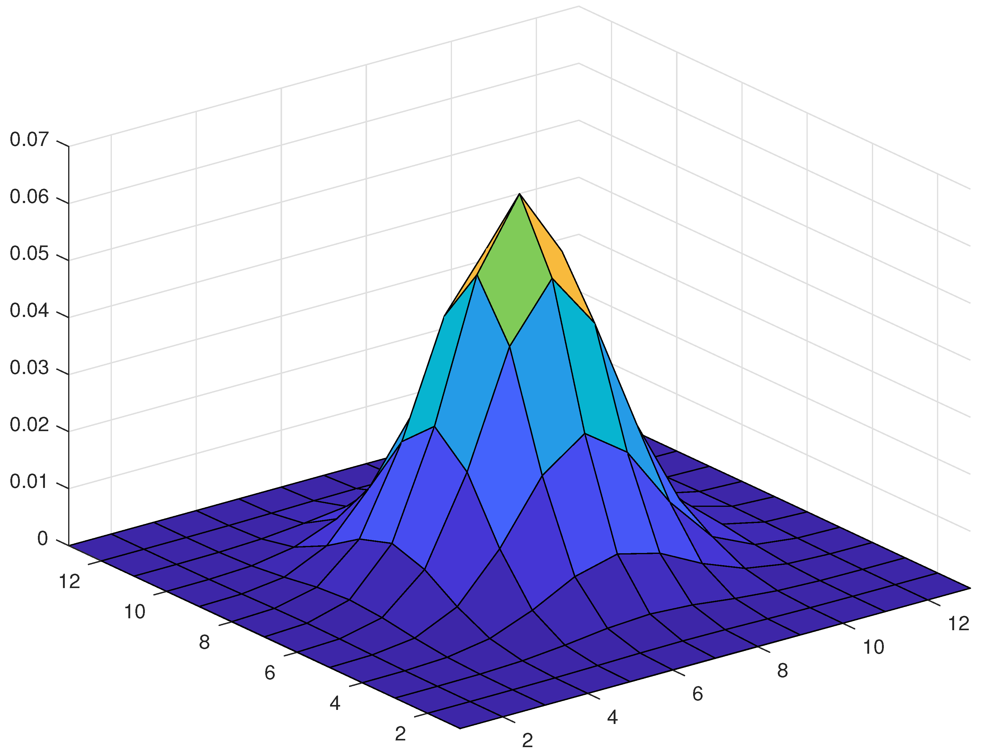
The weights of this two dimensional convolution are denoted by . If and is given by Equation (2), the shape of a weight is shown in Figure 1.
The main relation with one dimensional mollification is [4]:
2.4. Abstract Setting
The discrete convolutions that define mollification in one and two dimensions have their counterparts in infinite dimensions. It is true that in numerical computations, one deals with discrete functions, but what about the error estimates? They relate the abstract model based on differential equations with the discretized problem.
Convolutions are troublesome near borders; thus, whenever a convolution is mentioned, some kind of domain restriction is in order. Our presentation of the abstract setting follows Reference [17]. Let and If the two-dimensional truncated Gaussian kernel is defined by multiplication of the known one dimensional kernels, that is:
where This kernel satisfies:
- ,
- outside ,
- .
Definition 1.
A function is called Lipschitz continuous, if there exists a constant such that:
The next lemma establishes the consistency and stability of the two-dimensional discrete mollification.
Lemma 1.
Suppose g is a Lipschitz continuous function with Lipschitz constant L defined on I and is the associated discrete function defined on a uniform grid covering with step size h in both directions. Then, there exists a constant C such that:
- 1.
- Consistency
Proof.
This is Lemma 3.1 Part (1) of Reference [17]. □
Remark 1.
Notice that due to Equation (2), we may say that the right hand side bound is of the form , where C depends on , and η.
- 2.
- Stability: If is a Lipschitz continuous approximation of g so that , then:
Remark 2.
Actually, the right hand side bound is of the form , according to the previous remark.
Proof.
It follows from Part 1 that since:
where μ stands for measure. Notice that this estimate is valid in any other square subset of . Only the constant may change. □
3. The Inverse Source Problem
Fractional derivatives have been known since the seventeenth century, but only recently have they become the subject of attention due in part to a variety of interesting applications. Podlubny [18] says: “Fractional derivatives provide an excellent instrument for the description of memory and hereditary properties of various materials and processes.” We mention only two examples: For materials, we chose the damage evolution of brain tissue modeled in Reference [19] by a model in which the time derivative is a Caputo–Almeida fractional derivative. For processes, we selected the anomalous diffusion of a contaminant in fractured porous rocks modeled in Reference [20]. The model is based on fractional differentiation in the sense of Caputo.
3.1. Direct Problem
Our concern is a time fractional diffusion equation. More precisely, we are interested in an initial/boundary value problem, in which the time derivative is a Caputo fractional derivative of order The Caputo fractional derivative of order of a differentiable function v is:
where is the Gamma function given by:
We are interested in the following initial/boundary value problem:
where and:
The coefficients satisfy , (), , . The theoretical analysis that follows is from References [11,13,21]. The operator is a symmetric uniformly elliptic operator defined on .
The direct problem is to find u that safisfies Equation (13), with p and f known functions and a known fractional order of differentiation. If we think of this problem as the model for a contaminant diffusion in groundwater, then plays the role of contaminant discharge intensity and is an attenuation coefficient.
Let be the eigenvalues of , with associated eigenfunctions . It is known that and is an orthonormal basis of
The first step is the consideration of a fractional power operator and the space:
where is the inner product in . It is a Hilbert space with the norm:
The Mittag–Leffler function is a generalization of the exponential function and is very useful when dealing with fractional derivatives.
Definition 2.
A two-parameter function of the Mittag–Leffler type is defined by:
where are real constants and Γ is the Gamma function defined by Equation (12).
The formal solution of the direct problem (13) can be written in terms of a Mittag–Leffler function. It is:
where
3.2. Inverse Problem
We are interested in the inverse problem of determining the unknown source ingredient in Equation (13) based on the overposed data Time T is a final time and the data are not known exactly; what is known is a measurement so that
The operator K is a linear self-adjoint compact operator and Problem (19) is ill-posed.
Our aim is to obtain a function that minimizes the functional:
where is the mollification of a discrete version of the noisy data . Since K is a self-adjoint compact operator, there exists a minimizer of H, , given by:
Theorem 1.
Theorem 2.
Suppose satisfies . Moreover, suppose and there exist and E, a constant such that , then:
where depends on .
Proof.
The inequality follows from Theorem 1. However, , which implies . Taking , we obtain:
Following Reference [11] and taking into consideration Lemma 1, Part 1, we conclude:
□
4. Numerical Results
There are many alternatives for the numerical solution of a time fractional diffusion problem. If we restrict our attention to methods based on finite difference discretizations, we mention Reference [22], in which Caputo fractional derivatives are computed by the so-called Caputo fractional derivative rule, which in turn depends on a modified trapezoidal rule. This method is successfully implemented in Reference [23] for plane strain/stress elasticity in the presence of nonlocal elasticity.
Our finite difference method for the solution of the time fractional diffusion equation is taken from Reference [14], which in turn is inspired by Reference [24]. The method is implicit and its properties about stability and convergence are discussed in Reference [14].
We consider the following time fractional diffusion problem:
where:
After discretization, operator L leads to a matrix l, whose eigenvectors and eigenvalues play the roles of the eigenfunctions and eigenvalues of the differential operator.
The s are approximated according to Reference [11] by:
The integrals are approximated by composite trapezoidal rule.
The errors are measured by the root mean square (rms) norm given by:
The particular examples considered here are for:
The space step size is used for both coordinates, x and y. Final time is and .
Example 1
Example 2
5. Discussion and Final Comments
The 2DDM operator is a useful regularization procedure when dealing with inverse source problems for time fractional diffusion equations. It is also appropriate for surface and gradient fitting as shown in Reference [17], but we do not pursue this objective here. There are more applications of this operator and we hope to master some of them; for instance, we would like to modify our identification problem and deal with the factor as unknown and the factor as data.
Author Contributions
Conceptualization, M.E. and C.M.; Investigation, M.E. and C.M.; Writing—Original Draft Preparation, M.E. and C.M.; Writing—Review & Editing, M.E. and C.M.
Funding
Manuel D. Echeverry would like to thank COLCIENCIAS convocatoria-647 for financial support through a Ph.D. study grant.
Acknowledgments
The authors acknowledge the support provided by Universidad Nacional de Colombia through the research project Nonlocal operators and operators with memory, Hermes code number 33154.
Conflicts of Interest
The authors declare no conflict of interest.
References
- Acosta, C.D.; Mejía, C.E. Stable Computations by Discrete Mollification; Universidad Nacional de Colombia: Bogotá, Colombia, 2014. [Google Scholar]
- Murio, D.A. Mollification and Space Marching. In Inverse Engineering Handbook; Woodbury, K., Ed.; CRC Press: Boca Raton, FL, USA, 2002. [Google Scholar]
- Acosta, C.D.; Mejía, C.E. Stabilization of explicit methods for convection diffusion equations by discrete mollification. Comput. Math. Appl. 2008, 55, 368–380. [Google Scholar] [CrossRef]
- Acosta, C.D.; Buerger, R. Difference schemes stabilized by discrete mollification for degenerate parabolic equations in two space dimensions. IMA J. Numer. Anal. 2012, 32, 1509–1540. [Google Scholar] [CrossRef]
- Shi, C.; Wang, C.; Wei, T. Convolution regularization method for backward problems of linear parabolic equations. Appl. Numer. Math. 2016, 108, 143–156. [Google Scholar] [CrossRef]
- Garshasbi, M.; Dastour, H. Estimation of unknown boundary functions in an inverse heat conduction problem using a mollified marching scheme. Numer. Algorithms 2015, 68, 769–790. [Google Scholar] [CrossRef]
- Mejía, C.E.; Piedrahita, A. Solution of a time fractional inverse advection-dispersion problem by discrete mollification. Rev. Colomb. Mat. 2017, 51, 83–102. [Google Scholar] [CrossRef]
- Yang, F.; Fu, C.; Li, X. A mollification regularization method for unknown source in time-fractional diffusion equation. Int. J. Comput. Mat. 2014, 91, 1516–1534. [Google Scholar] [CrossRef]
- Beatson, R.; Bui, H.Q. Mollification formulas and implicit smoothing. Adv. Comput. Mat. 2007, 27, 125–149. [Google Scholar] [CrossRef]
- Yi, Z.; Murio, D.A. Identification of Source Terms in 2-D IHCP. Comput. Math. Appl. 2004, 47, 1517–1533. [Google Scholar] [CrossRef]
- Ma, Y.; Prakash, P.; Deiveegan, A. Generalized Tikhonov methods for an inverse source problem of the time-fractional diffusion equation. Chaos Solitons Fract. 2018, 108, 39–48. [Google Scholar] [CrossRef]
- Nguyen, H.T.; Le, D.L.; Nguyen, V.T. Regularized solution of an inverse source problem for a time fractional diffusion equation. Appl. Math. Model. 2016, 40, 8244–8264. [Google Scholar] [CrossRef]
- Wei, T.; Wang, J. A modified quasi-boundary value method for an inverse source problem of the time-fractional diffusion equation. Appl. Numer. Math. 2014, 78, 95–111. [Google Scholar] [CrossRef]
- Mejía, C.E.; Piedrahita, A. A finite difference approximation of a two dimensional time fractional advection-dispersion problem. arXiv 2018, arXiv:1807.07393v1. [Google Scholar]
- Sakamoto, K.; Yamamoto, M. Inverse source problem with a final overdetermination for a fractional diffusion equation. Math. Control Relat. Fields 2011, 1, 509–518. [Google Scholar] [CrossRef] [Green Version]
- Jiang, D.; Li, Z.; Liu, Y.; Yamamoto, M. Weak unique continuation property and a related inverse source problem for time-fractional diffusion-advection equations. Inverse Probl. 2017, 33, 055013. [Google Scholar] [CrossRef] [Green Version]
- Zhan, S.; Murio, D.A. Surface fitting and numerical gradient computation by discrete mollification. Comput. Math. Appl. 1999, 37, 145–159. [Google Scholar] [CrossRef]
- Podlubny, I. Fractional Differential Equations; Academic Press: Cambridge, MA, USA, 1999. [Google Scholar]
- Voyiadjis, G.Z.; Sumelka, W. Brain modelling in the framework of anisotropic hyperelasticity with time fractional damage evolution governed by the Caputo-Almeida fractional derivative. J. Mech. Behav. Biomed. Mater. 2019, 89, 209–216. [Google Scholar] [CrossRef] [PubMed]
- Fomin, S.; Chugunov, V.; Hashida, T. Application of fractional differential equations for modeling the anomalous diffusion of contaminant from fracture into porous rock matrix with bordering alteration zone. Transp. Porous Med. 2010, 81, 187–205. [Google Scholar] [CrossRef]
- Sakamoto, K.; Yamamoto, M. Initial value/boundary value problems for fractional diffusion-wave equations and applications to some inverse problems. J. Math. Anal. Appl. 2011, 382, 426–447. [Google Scholar] [CrossRef]
- Odibat, Z. Approximations of fractional integrals and Caputo fractional derivatives. Appl. Math. Comput. 2006, 178, 527–533. [Google Scholar] [CrossRef]
- Sumelka, W.; Szajek, K.; Lodygowski, T. Plain strain and plane stress elasticity under fractional continuum mechanics. Arch. Appl. Mech. 2015, 85, 1527–1544. [Google Scholar] [CrossRef]
- Zhuang, P.; Liu, F. Finite difference approximation for two-dimensional time fractional diffusion equation. J. Algorithms Comput. Technol. 2007, 1, 1–16. [Google Scholar] [CrossRef] [Green Version]
Figure 1.
A weight for and .

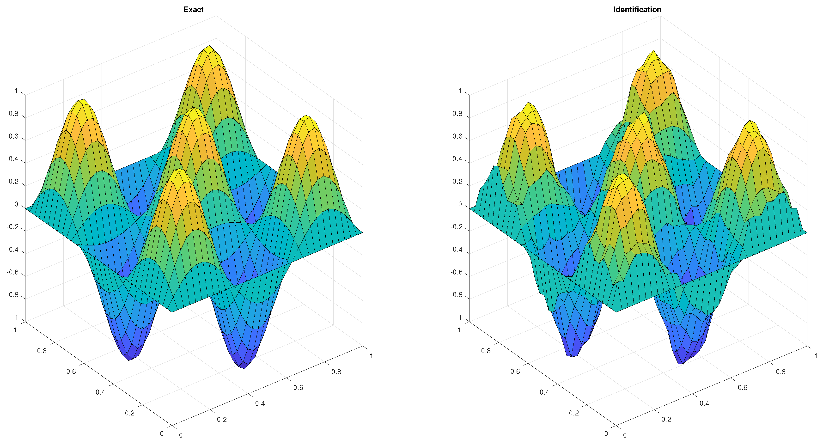
Figure 2.
Identification of f for and .


Table 1.
Mollification weights.
| 1 | 8.4272 | 7.8640 | ||||
| 2 | 6.0387 | 1.9262 | 5.4438 | |||
| 3 | 4.5556 | 2.3772 | 3.3291 | 1.2099 | ||
| 4 | 3.6266 | 2.4003 | 6.9440 | 8.7275 | 4.7268 | |
| 5 | 3.0028 | 2.2625 | 9.6723 | 2.3430 | 3.2095 | 2.4798 |
Table 2.
Error norms, and .
| 0.1 | 0.5 | 0.7 | 0.9 | |
|---|---|---|---|---|
| 0.11237258 | 0.11341573 | 0.11482934 | 0.11338589 |
Table 3.
Error norms, .
| 0.005 | 0.01 | 0.025 | 0.05 | |
|---|---|---|---|---|
| 3 | 4 | 5 | 6 | |
| 0.05634342 | 0.11141561 | 0.17683141 | 0.24996681 |
Table 4.
Error norms, and .
| 0.1 | 0.5 | 0.7 | 0.9 | |
|---|---|---|---|---|
| 0.18679846 | 0.18330355 | 0.19129097 | 0.19253567 |
Table 5.
Error norms, .
| 0.005 | 0.01 | 0.025 | 0.05 | |
|---|---|---|---|---|
| 3 | 4 | 5 | 6 | |
| 0.0715818 | 0.12090887 | 0.19295488 | 0.26167402 |
© 2018 by the authors. Licensee MDPI, Basel, Switzerland. This article is an open access article distributed under the terms and conditions of the Creative Commons Attribution (CC BY) license (http://creativecommons.org/licenses/by/4.0/).
Share and Cite
MDPI and ACS Style
Echeverry, M.D.; Mejía, C.E. A Two Dimensional Discrete Mollification Operator and the Numerical Solution of an Inverse Source Problem. Axioms 2018, 7, 89. https://doi.org/10.3390/axioms7040089
AMA Style
Echeverry MD, Mejía CE. A Two Dimensional Discrete Mollification Operator and the Numerical Solution of an Inverse Source Problem. Axioms. 2018; 7(4):89. https://doi.org/10.3390/axioms7040089
Chicago/Turabian StyleEcheverry, Manuel D., and Carlos E. Mejía. 2018. "A Two Dimensional Discrete Mollification Operator and the Numerical Solution of an Inverse Source Problem" Axioms 7, no. 4: 89. https://doi.org/10.3390/axioms7040089
Note that from the first issue of 2016, this journal uses article numbers instead of page numbers. See further details here.