First Order Coupled Systems With Functional and Periodic Boundary Conditions: Existence Results and Application to an SIRS Model

Abstract

The results presented in this paper deal with the existence of solutions of a first order fully coupled system of three equations, and they are split in two parts: 1. Case with coupled functional boundary conditions, and 2. Case with periodic boundary conditions. Functional boundary conditions, which are becoming increasingly popular in the literature, as they generalize most of the classical cases and in addition can be used to tackle global conditions, such as maximum or minimum conditions. The arguments used are based on the Arzèla Ascoli theorem and Schauder’s fixed point theorem. The existence results are directly applied to an epidemic SIRS (Susceptible-Infectious-Recovered-Susceptible) model, with global boundary conditions.

1. Introduction

In this paper two different problems are analyzed.

Part one is concerned with the study of a fully nonlinear coupled system of equations

$$\left\{\begin{array}{c}{u}_1^{\prime }\left(t\right)=f_1\left(t,u_1\left(t\right),u_2\left(t\right),u_3\left(t\right)\right)\\ u_2^{\prime }\left(t\right)=f_2\left(t,u_1\left(t\right),u_2\left(t\right),u_3\left(t\right)\right)\\ u_3^{\prime }\left(t\right)=f_3\left(t,u_1\left(t\right),u_2\left(t\right),u_3\left(t\right)\right)\end{array}\right.,$$

(1)

$f_i:[a,b]\times {\mathbb{R}}^3\to \mathbb{R}$ and $i=1,2,3$ are $L^1—$Carathéodory functions, subject to the nonlinear functional boundary conditions

$$\begin{array}{c}{u}_1\left(a\right)=L_1\left(u_1,u_2,u_3,u_1\left(b\right),u_2\left(b\right),u_3\left(b\right),u_2\left(a\right),u_3\left(a\right)\right)\\ u_2\left(a\right)=L_2\left(u_1,u_2,u_3,u_1\left(b\right),u_2\left(b\right),u_3\left(b\right),u_1\left(a\right),u_3\left(a\right)\right)\\ u_3\left(a\right)=L_3\left(u_1,u_2,u_3,u_1\left(b\right),u_2\left(b\right),u_3\left(b\right),u_1\left(a\right),u_2\left(a\right)\right)\end{array}$$

(2)

where $L_i:{\left(C[a,b]\right)}^3\times {\mathbb{R}}^5\to \mathbb{R}$, $i=1,2,3,$ are continuous functions with properties later to be defined. The technique used for the functional problem is based on the Arzèla-Ascoli theorem and Schauder’s fixed point theorem.

Part two, more precisely, Section 4, deals with the fully nonlinear couple system of Equation (1) coupled with the periodic boundary conditions

$$\begin{array}{c}{u}_1\left(a\right)=u_1\left(b\right)\\ u_2\left(a\right)=u_2\left(b\right)\\ u_3\left(a\right)=u_3\left(b\right).\end{array}$$

(3)

Given that the conditions on $L_i$, do not allow the problem (1)–(2) to cover the periodic case, a different approach for the problem (1)–(3) is required. In this case, in order to obtain the existence and location of periodic solutions, the upper and lower solutions method, along with some adequate local monotone assumptions on the nonlinearities, is used.

Mathematical modelling and applications are becoming increasingly popular nowadays. With the sudden outburst of keywords such as big data, data analytics and modelling, the quest for mathematical models is on high demand. In the area of mathematical modelling, systems of differential equations are a must, due to their high applicability in areas such as population dynamics [1,2,3], finance [4], medicine [5], biotechnology [6] and physics [7,8], and also examples treated in [9,10].

Nevertheless, in the literature available, the cases dealing with coupled systems of equations are not abundant. Such systems can be found in [11,12,13], however, in this paper the authors present a problem where both equations are coupled. In addition to that, to the best of our knowledge, it is the first time where coupled systems are considered with coupled functional boundary conditions.

This feature allows to generalize the classical boundary data in the literature, such as two-point or multi-point, nonlinear, nonlocal, integro-differential conditions, among others. Indeed, the functional part can deal with global boundary assumptions, such as minimum or maximum arguments, infinite multi-point data, and integral conditions on the several unknown functions. Functional problems, along with their features, can be seen in [14,15,16,17,18,19] and the references therein.

The methods and techniques applied in this paper can be easily adapted to coupled systems with n equations and variables. However, as the notation and writing appear to be heavy, and may avoid the clarity of the results, we prefer to prove our theoretical part for $n=3,$ which is adequate for our application.

This paper has the following structure: Section 2 contains some definitions and generic assumptions on the nonlinearities. Section 3 shows the main result for problems with functional boundary conditions. In Section 4 it is studied the periodic problem via lower and upper solutions technique together with some local growth conditions. The final section presents an application of (1)–(2) to an epidemic SIRS model to illustrate the applicability of the problem discussed and to show the potentialities of the functional boundary conditions, exploring global initial boundary conditions on the system.

2. Definitions and Assumptions

Throughout this work we consider the space of continuous functions in $[a,b]$, on the Banach space $E:={\left(C[a,b]\right)}^3,$ equipped with the norm

$${∥u∥}_E=max\left\{∥u_i∥,i=1,2,3\right\}$$

where $∥u_i∥={max}_{t\in \left[a,b\right]}\left|u_i\left(t\right)\right|$.

The functional boundary functions verify the assumption:

Hypothesis 1.

$L_i:{\left(C[a,b]\right)}^3\times {\mathbb{R}}^5\to \mathbb{R}$are continuous functions. Moreover, each of the functions,$L_i\left(\eta ,x,y\right)$are uniformly continuous when$\left(\eta ,x,y\right)$is bounded.

The admissible nonlinearities will be $L^1—$Carathéodory functions, according the following definition:

Definition 1.

The functions$f_i:[a,b]\times {\mathbb{R}}^3\to \mathbb{R},$$i=1,\dots ,n,$are$L^1—$Carathéodory if they verify:

(i) 

for each$\left(y_1,y_2,y_3\right)\in {\mathbb{R}}^3$,$t\mapsto f_i(t,y_1,y_2,y_3)$are measurable on$[a,b],$for$i=1,2,3;$

(ii) 

for almost every$t\in [a,b],$$\left(y_1,y_2,y_3\right)\mapsto f_i(t,y_1,y_2,y_3)$are continuous on${\mathbb{R}}^3,$for$i=1,2,3;$

(iii) 

for each$L>0$, there exists a positive function${\psi }_{iL}\in L^1\left[a,b\right],$$i=1,2,3,$such that, for$max\left\{∥y_i∥,i=1,2,3\right\}<L$,

$$\left|f_i(t,y_1\left(t\right),y_2\left(t\right),y_3\left(t\right))\right|\le {\psi }_{iL}\left(t\right),a.e.t\in [a,b],i=1,2,3.$$

To demonstrate the final result, Schauder’s fixed point theorem will be an important tool to guarantee the existence of fixed points for the operator to be defined:

Theorem 1.

([20]) Let Y be a nonempty, closed, bounded and convex subset of a Banach space X, and suppose that$P:Y\to Y$is a completely continuous operator. Then P has at least one fixed point in Y.

3. Main Result for Functional Problems

In this section, we present and prove the main existence result for (1)–(2), given by the following theorem:

Theorem 2.

If$f_i$are$L^1—$Carathéodory functions, for$i=1,2,3,$and the continuous functions$L_i,$$i=1,2,3,$verify (H1) and

Hypothesis 2.

there exists$R>0$such that

$$\underset{}{max}\left\{k_i+{\int }_a^t{\psi }_{iR}\left(s\right)ds,i=1,2,3\right\}\le R,$$

with

$$\begin{array}{c}{k}_1:=max\left\{L_1\left(u_1,u_2,u_3,u_1\left(b\right),u_2\left(b\right),u_3\left(b\right),u_2\left(a\right),u_3\left(a\right)\right)\right\},\\ k_2:=max\left\{L_2\left(u_1,u_2,u_3,u_1\left(b\right),u_2\left(b\right),u_3\left(b\right),u_1\left(a\right),u_3\left(a\right)\right)\right\},\\ k_3:=max\left\{L_3\left(u_1,u_2,u_3,u_1\left(b\right),u_2\left(b\right),u_3\left(b\right),u_1\left(a\right),u_2\left(a\right)\right)\right\},\end{array}$$

then the problem (1)–(2) has at least one solution$u=(u_1,u_2,u_3)\in {\left(C\left[a,b\right]\right)}^3.$

Proof. 

Let us consider the integral system given by

$$\left\{\begin{array}{c}{u}_1\left(t\right)=L_1\left(u_1,u_2,u_3,u_1\left(b\right),u_2\left(b\right),u_3\left(b\right),u_2\left(a\right),u_3\left(a\right)\right)+{\int }_a^t{f}_1\left(s,u_1\left(s\right),u_2\left(s\right),u_3\left(s\right)\right)ds,\\ u_2\left(t\right)=L_2\left(u_1,u_2,u_3,u_1\left(b\right),u_2\left(b\right),u_3\left(b\right),u_1\left(a\right),u_3\left(a\right)\right)+{\int }_a^t{f}_2\left(s,u_1\left(s\right),u_2\left(s\right),u_3\left(s\right)\right)ds,\\ u_3\left(t\right)=L_3\left(u_1,u_2,u_3,u_1\left(b\right),u_2\left(b\right),u_3\left(b\right),u_1\left(a\right),u_2\left(a\right)\right)+{\int }_a^t{f}_3\left(s,u_1\left(s\right),u_2\left(s\right),u_3\left(s\right)\right)ds,\end{array}\right.$$

(4)

and the operator

$$T:{\left(C\left[a,b\right]\right)}^3\to {\left(C\left[a,b\right]\right)}^3$$

defined by

$$T\left(u_1,u_2,u_3\right)=\left(T_1\left(u_1,u_2,u_3\right),T_2\left(u_1,u_2,u_3\right),T_3\left(u_1,u_2,u_3\right)\right),$$

(5)

where $T_i:{\left(C\left[a,b\right]\right)}^3\to C\left[a,b\right],$ $i=1,2,3,$ given by

$$\begin{array}{c}{T}_1\left(u_1,u_2,u_3\right)=L_1\left(u_1,u_2,u_3,u_1\left(b\right),u_2\left(b\right),u_3\left(b\right),u_2\left(a\right),u_3\left(a\right)\right)+{\int }_a^t{f}_1\left(s,u_1\left(s\right),u_2\left(s\right),u_3\left(s\right)\right)ds,\\ T_2\left(u_1,u_2,u_3\right)=L_2\left(u_1,u_2,u_3,u_1\left(b\right),u_2\left(b\right),u_3\left(b\right),u_1\left(a\right),u_3\left(a\right)\right)+{\int }_a^t{f}_2\left(s,u_1\left(s\right),u_2\left(s\right),u_3\left(s\right)\right)ds,\\ T_3\left(u_1,u_2,u_3\right)=L_3\left(u_1,u_2,u_3,u_1\left(b\right),u_2\left(b\right),u_3\left(b\right),u_1\left(a\right),u_2\left(a\right)\right)+{\int }_a^t{f}_3\left(s,u_1\left(s\right),u_2\left(s\right),u_3\left(s\right)\right)ds,\end{array}$$

(6)

As the fixed points of T are fixed points of $T_i,$ $i=1,2,3,$ and vice-versa, which are solutions of (1)–(2), the goal of this architecture will be to use the Arzèla-Ascoli theorem and Schauder’s fixed point theorem to prove that the problem (1)–(2) has at least one solution.

For clarity, we consider several claims:

Claim 1.

$TD\subset D$, for some$D\subset {\left(C\left[a,b\right]\right)}^3$a bounded, closed and convex subset.

Consider

$$D=\left\{\left(u_1,u_2,u_3\right)\in {\left(C\left[a,b\right]\right)}^3:{∥\left(u_1,u_2,u_3\right)∥}_E\le k\right\},$$

with $k>0$ such that

$$\underset{}{max}\left\{k_i+{\int }_a^t{\psi }_{ik}\left(s\right)ds,i=1,2,3\right\}\le k.$$

Given $\left(u_1,u_2,u_3\right)\in D$, by Definition 1 (iii) and (Hypothesis 2), we have that for $\left(u_1,u_2,u_3\right)\in D,$ $i=1,2,3,$

$$\left|f_i\left(s,u_1\left(s\right),u_2\left(s\right),u_3\left(s\right)\right)\right|\le {\psi }_{ik}\left(s\right),a.e.s\in \left[a,b\right].$$

Therefore, ${∥T\left(u_1,u_2,u_3\right)∥}_E\le k$ and Claim 1 is proved.

Claim 2.

The operator T is completely continuous.

To prove that the operator T is completely continuous it is sufficient to show that T is uniformly bounded and T is equicontinuous. Using the above arguments, it can be proved that $T_i$ are uniformly bounded, for $i=1,2,3,$ and therefore T is uniformly bounded.

In order to show that the operator T is equicontinuous, let us consider $t_1,t_2\in \left[a,b\right]$, such that, without any loss of generality, $t_1<t_2.$

Then for $T_i,$ $i=1,2,3,$ we have

$$\begin{array}{l}\left|T_i\left(u_1\left(t_2\right),u_2\left(t_2\right),u_3\left(t_2\right)\right)-T_i\left(u_1\left(t_1\right),u_2\left(t_1\right),u_3\left(t_1\right)\right)\right|\\ \le {\int }_{t_1}^{t_2}\left|f_i\left(s,u_1\left(s\right),u_2\left(s\right),u_3\left(s\right)\right)\right|ds\le {\int }_{t_1}^{t_2}{\psi }_{iL}\left(s\right)ds\to 0,\end{array}$$

as $t_1\to t_2.$ So, each operator $T_i$ is equicontinuous and, hence, the operator T is equicontinuous.

Therefore, by Arzèla-Ascoli’s theorem, the operator T is compact and using Schauder’s fixed point theorem, we obtain that T has a fixed point, that is, the problem (1)–(2) has at least a solution $u\in {\left(C\left[a,b\right]\right)}^3.$ □

Remark that (Hypothesis 2) implies that the periodic case is not covered by (2).

4. Existence and Localization Result for the Periodic Case

Consider now the system (1) with the periodic boundary conditions (3). As it is well known, in nonlinear differential equations, the periodic case is more delicate and requires a different approach for general nonlinearities.

The method to be used will apply lower and upper solutions technique, based on the definition:

Definition 2.

Consider the$C^1$-functions${\alpha }_i,{\beta }_i:\left[a,b\right]\to \mathbb{R},$$i=1,2,3.$The triple$\left({\alpha }_1,{\alpha }_2,{\alpha }_3\right)$is a lower solution of the periodic problem (1), (3) if

$$\left\{\begin{array}{c}{\alpha }_1^{\prime }\left(t\right)\le f_1\left(t,{\alpha }_1\left(t\right),{\alpha }_2\left(t\right),{\alpha }_3\left(t\right)\right)\\ {\alpha }_2^{\prime }\left(t\right)\le f_2\left(t,{\alpha }_1\left(t\right),{\alpha }_2\left(t\right),{\alpha }_3\left(t\right)\right)\\ {\alpha }_3^{\prime }\left(t\right)\le f_3\left(t,{\alpha }_1\left(t\right),{\alpha }_2\left(t\right),{\alpha }_3\left(t\right)\right)\end{array}\right.$$

(7)

and

$$\begin{array}{c}{\alpha }_1\left(a\right)\le {\alpha }_1\left(b\right)\\ {\alpha }_2\left(a\right)\le {\alpha }_2\left(b\right)\\ {\alpha }_3\left(a\right)\le {\alpha }_3\left(b\right).\end{array}$$

(8)

The triple$\left({\beta }_1,{\beta }_2,{\beta }_3\right)$is an upper solution of the periodic problem (1), (3) if the reversed inequalities hold.

This method allows to obtain an existence and localization theorem:

Theorem 3.

Let$\left({\alpha }_1,{\alpha }_2,{\alpha }_3\right)$and$\left({\beta }_1,{\beta }_2,{\beta }_3\right)$be lower and upper solutions of (1), (3), respectively, such that${\alpha }_i\left(t\right)\le {\beta }_i\left(t\right),$$\forall t\in \left[a,b\right]$and for$i=1,2,3.$

Define the set

$$A=\left\{\left(t,u_1,u_2,u_3\right)\in \left[a,b\right]\times {\mathbb{R}}^3:{\alpha }_i\left(t\right)\le u_i\le {\beta }_i\left(t\right),i=1,2,3\right\}$$

and assume that$f_i$are$L^1—$Carathéodory functions on A, for$i=1,2,3$verifying

$$f_1\left(t,x,{\alpha }_2\left(t\right),{\alpha }_3\left(t\right)\right)\le f_1\left(t,x,y,z\right)\le f_1\left(t,x,{\beta }_2\left(t\right),{\beta }_3\left(t\right)\right),$$

(9)

for$t\in \left[a,b\right],{\alpha }_2\left(t\right)\le y\le {\beta }_2\left(t\right),{\alpha }_3\left(t\right)\le z\le {\beta }_3\left(t\right),$

$$f_2\left(t,{\alpha }_1\left(t\right),y,{\alpha }_3\left(t\right)\right)\le f_2\left(t,x,y,z\right)\le f_2\left(t,{\beta }_1\left(t\right),y,{\beta }_3\left(t\right)\right),$$

for$t\in \left[a,b\right],{\alpha }_1\left(t\right)\le x\le {\beta }_1\left(t\right),{\alpha }_3\left(t\right)\le z\le {\beta }_3\left(t\right),$

$$f_3\left(t,{\alpha }_1\left(t\right),{\alpha }_2\left(t\right),z\right)\le f_3\left(t,x,y,z\right)\le f_3\left(t,{\beta }_1\left(t\right),{\beta }_2\left(t\right),z\right),$$

for$t\in \left[a,b\right],{\alpha }_1\left(t\right)\le x\le {\beta }_1\left(t\right),{\alpha }_2\left(t\right)\le y\le {\beta }_2\left(t\right).$

Then the problem (1), (3) has, at least, a solution$u=(u_1,u_2,u_3)\in {\left(C\left[a,b\right]\right)}^3$such that

$${\alpha }_i\left(t\right)\le u_i\left(t\right)\le {\beta }_i\left(t\right),i=1,2,3,\mathit{for}\mathit{all}t\in \left[a,b\right].$$

Proof. 

For $i=1,2,3,$ define the truncature functions ${\delta }_i$ given by

$${\delta }_i(t,u_i)=\left\{\begin{array}{ccc}{\alpha }_i\left(t\right)& \mathrm{if}& u_i<{\alpha }_i\left(t\right)\\ u_i& \mathrm{if}& {\alpha }_i\left(t\right)\le u_i\le {\beta }_i\left(t\right)\\ {\beta }_i\left(t\right)& \mathrm{if}& u_i>{\beta }_i\left(t\right)\end{array}\right.$$

and consider the modified problem composed by the truncated and perturbed differential equations

$$\left\{\begin{array}{c}{u}_1^{\prime }\left(t\right)+u_1\left(t\right)=f_1\left(t,{\delta }_1(t,u_1),{\delta }_2(t,u_2),{\delta }_3(t,u_3)\right)+{\delta }_1(t,u_1)\\ u_2^{\prime }\left(t\right)+u_2\left(t\right)=f_2\left(t,{\delta }_1(t,u_1),{\delta }_2(t,u_2),{\delta }_3(t,u_3)\right)+{\delta }_2(t,u_2)\\ u_3^{\prime }\left(t\right)+u_3\left(t\right)=f_3\left(t,{\delta }_1(t,u_1),{\delta }_2(t,u_2),{\delta }_3(t,u_3)\right)+{\delta }_3(t,u_3),\end{array}\right.$$

(10)

together with the boundary conditions (3).

As the linear and homogeneous problem associated to (10), (3) has only the null solution, then we can write (10), (3) in the integral form

$$\left\{\begin{array}{l}{u}_1\left(t\right)={\int }_a^b{G}_1(t,s)\left[\begin{array}{c}{f}_1\left(s,{\delta }_1(s,u_1\left(s\right)),{\delta }_2(s,u_2\left(s\right)),{\delta }_3(s,u_3\left(s\right))\right)\\ +{\delta }_1(s,u_1\left(s\right))\end{array}\right]ds\\ u_2\left(t\right)={\int }_a^b{G}_2(t,s)\left[\begin{array}{c}{f}_2\left(s,{\delta }_1(s,u_1\left(s\right)),{\delta }_2(s,u_2\left(s\right)),{\delta }_3(s,u_3\left(s\right))\right)\\ +{\delta }_2(s,u_2\left(s\right))\end{array}\right]ds\\ u_3\left(t\right)={\int }_a^b{G}_3(t,s)\left[\begin{array}{c}{f}_3\left(s,{\delta }_1(s,u_1\left(s\right)),{\delta }_2(s,u_2\left(s\right)),{\delta }_3(s,u_3\left(s\right))\right)\\ +{\delta }_3(s,u_3\left(s\right))\end{array}\right]ds,\end{array}\right.$$

(11)

where $G_i(t,s)$ are the Green functions corresponding to the problem

$$\begin{array}{rrr}{u}_i^{\prime }\left(t\right)+u_i\left(t\right)& =& f_i\left(t\right)\\ u_i\left(a\right)& =& u_i\left(b\right),\end{array}$$

for $i=1,2,3.$

Then the operator

$$T:{\left(C\left[a,b\right]\right)}^3\to {\left(C\left[a,b\right]\right)}^3$$

given by

$$T\left(u_1,u_2,u_3\right)=\left(T_1\left(u_1,u_2,u_3\right),T_2\left(u_1,u_2,u_3\right),T_3\left(u_1,u_2,u_3\right)\right),$$

with $T_i:{\left(C\left[a,b\right]\right)}^3\to C\left[a,b\right],$ $i=1,2,3,$ defined as

$$\begin{array}{c}{T}_1\left(u_1,u_2,u_3\right)={\int }_a^b{G}_1(t,s)\left[\begin{array}{c}{f}_1\left(s,{\delta }_1(s,u_1\left(s\right)),{\delta }_2(s,u_2\left(s\right)),{\delta }_3(s,u_3\left(s\right))\right)\\ +{\delta }_1(s,u_1\left(s\right))\end{array}\right]ds\\ T_2\left(u_1,u_2,u_3\right)={\int }_a^b{G}_2(t,s)\left[\begin{array}{c}{f}_2\left(s,{\delta }_1(s,u_1\left(s\right)),{\delta }_2(s,u_2\left(s\right)),{\delta }_3(s,u_3\left(s\right))\right)\\ +{\delta }_2(s,u_2\left(s\right))\end{array}\right]ds\\ T_3\left(u_1,u_2,u_3\right)={\int }_a^b{G}_3(t,s)\left[\begin{array}{c}{f}_3\left(s,{\delta }_1(s,u_1\left(s\right)),{\delta }_2(s,u_2\left(s\right)),{\delta }_3(s,u_3\left(s\right))\right)\\ +{\delta }_3(s,u_3\left(s\right))\end{array}\right]ds\end{array}$$

is completely continuous in ${\left(C\left[a,b\right]\right)}^3.$

By Schauder’s fixed point theorem, we obtain that T has a fixed point, that is, the problem (10), (3) has at least a solution $u_{\ast }:=\left(u_{\ast 1},u_{\ast 2},u_{\ast 3}\right)\in {\left(C\left[a,b\right]\right)}^3.$

To prove that this function $u_{\ast }$ is a solution of the initial problem (1), (3), it will be enough to show that

$${\alpha }_i\left(t\right)\le u_{\ast i}\left(t\right)\le {\beta }_i\left(t\right),i=1,2,3,\mathrm{for}\mathrm{all}t\in \left[a,b\right].$$

Suppose that the first inequality does not hold for $i=1$ and some $t_1\in \left[a,b\right],$ that is

$$u_{\ast 1}\left(t_1\right)<{\alpha }_1\left(t_1\right).$$

Extend the function $u_{\ast 1}-{\alpha }_1$ by periodicity and consider

$$t_0:=inf\left\{t\in \left[t_1-b+a,t_1\right]:\forall s\in ]t,t_1],u_{\ast 1}\left(s\right)<{\alpha }_1\left(s\right)\right\}.$$

Therefore, for $t\in [t_0,t_1]$ we have, by Definition 2 and (9),

$$\begin{array}{l}{u}_{\ast 1}^{\prime }\left(t\right)-{\alpha }_1^{\prime }\left(t\right)\\ \ge f_1\left(t,{\alpha }_1\left(t\right),{\delta }_2(t,u_2),{\delta }_3(t,u_3)\right)+{\alpha }_1\left(t\right)-u_{\ast 1}\left(t\right)-f_1\left(t,{\alpha }_1\left(t\right),{\alpha }_2\left(t\right),{\alpha }_3\left(t\right)\right)\\ \ge {\alpha }_1\left(t\right)-u_{\ast 1}\left(t\right)>0.\end{array}$$

So, ${\alpha }_1-u_{\ast 1}$ is increasing on $\left[t_0,t_1\right]$ and

$$0>u_{\ast 1}\left(t_1\right)-{\alpha }_1\left(t_1\right)>u_{\ast 1}\left(t_0\right)-{\alpha }_1\left(t_0\right),$$

where $t_0=t_1-b+a,$ which is in contradiction of the periodicity of the extension of $u_{\ast 1}-{\alpha }_1.$ So ${\alpha }_1\left(t\right)\le u_{\ast 1}\left(t\right),$ for all $t\in \left[a,b\right].$

Applying similar arguments it can be proved that $u_{\ast 1}\left(t\right)\le {\beta }_1\left(t\right),$ for $t\in \left[a,b\right],$ and

$${\alpha }_i\left(t\right)\le u_{\ast i}\left(t\right)\le {\beta }_i\left(t\right),i=2,3,\mathrm{for}\mathrm{all}t\in \left[a,b\right].$$

 □

5. An Epidemic Model of an SIRS System With Nonlinear Incidence Rate and Interaction from Infectious to Susceptible Subjects

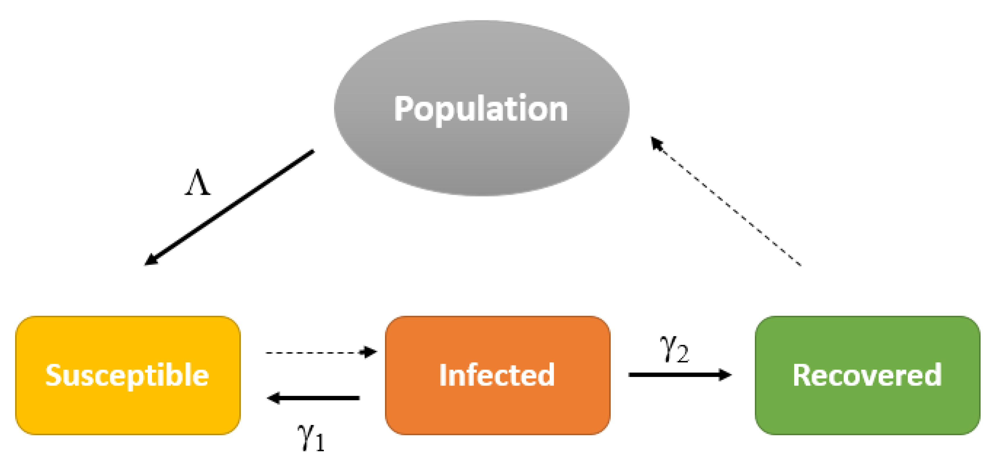
The existent literature has innumerous examples of applications of SIR models, namely in [21,22,23] where the population is divided into Susceptible $\left(S\right)$, Infectious $\left(I\right)$ and Recovery $\left(R\right).$ However, in SIR models, recovered individuals are assumed to develop lifelong immunity, which for some diseases such as seasonal flu, influenza or venereal diseases is not necessarily true. A recovered individual becomes susceptible and possibly infected after some time. In this case, SIRS models, where recovered individuals lose immunity and become susceptible again, are far more adequate. Examples can be found in [24,25,26,27,28,29]. In [30], the authors develop and explore a mathematical model of an SIRS epidemic model where a transfer between infectious and susceptible rate is included, as shown in Figure 1.

This approach was designed to model the cases where recovery cannot generate immunity for a long time. Infected individuals may recover after some treatments and go back directly to the susceptible class. In addition, a nonlinear incidence with the average number of new cases of a disease per unit time, $Sg\left(I\right),$ is included, as suggested in [31]. This nonlinear incidence replicates a more complex dynamic than the ones presented on bilinear or standard incidence models, and it seems to perform better when modelling more complex cholera cases, as shown in [31].

The model presented is then

$$\left\{\begin{array}{l}\frac{dS}{dt}=\frac{1}{100}\left(\mathsf{\Lambda }-\mu S-Sg\left(I\right)+{\gamma }_{1}I+\delta R\right),\\ \frac{dI}{dt}=\frac{1}{100}\left[Sg\left(I\right)-\left(\mu +{\gamma }_1+{\gamma }_2+\alpha \right)I\right],\\ \frac{dR}{dt}=\frac{1}{100}\left[{\gamma }_{2}I-\left(\mu +\delta \right)R\right]\end{array}\right.$$

(12)

where:

• $\mathsf{\Lambda }$ represents the recruitment rate of susceptible individuals;
• $\mu$ is the natural death rate;
• ${\gamma }_1$ is the transfer rate from the infected class to the susceptible class;
• ${\gamma }_2$ is the transfer rate from the infected class to the recovered class;
• $\alpha$ is the disease-induced death rate;
• $\delta$ the immunity loss rate.

In this model $\mathsf{\Lambda }$ and $\mu$ are assumed to be positive and $\delta ,$ ${\gamma }_1,$ ${\gamma }_2$ and $\alpha$ are assumed to be nonnegative. As per the nonlinear incidence, $Sg\left(I\right)$, g is a real locally Lipschitz function on ${\mathbb{R}}^{+}$ with the following conditions, as presented in [32]:

• $g\left(0\right)=0$ and $g\left(I\right)>0$ for $I>0,$
• $g\left(I\right)/I$ is continuous and monotonously increasing for $I>0$ and ${lim}_{I\to 0^{+}}\frac{g\left(I\right)}{I}$ exists as $\beta >0.$

Unlike the previous models presented, in this paper we couple the system (12) with the boundary conditions, for $t\in \left[0,T\right]$ and $T>0,$

$$\begin{array}{c}S\left(0\right)=\underset{t\in \left[0,T\right]}{max}I\left(t\right),\\ I\left(0\right)={\int }_0^{T}S\left(T\right)S\left(s\right)ds,\\ R\left(0\right)={\int }_0^{T}S\left(T\right)I\left(s\right)ds.\end{array}$$

(13)

These functional boundary conditions fully reflect the considerations and conclusions presented in [30]. These types of boundary conditions have the following practical meaning:

• $S\left(0\right)$, the initial number of susceptible subjects, is equal to the maximum of the infected subjects;
• $I\left(0\right),$ the initial number of infected subjects, is a weighted average of the susceptible individuals, weighted by the final value of the susceptible S, at time $T;$
• $R\left(0\right),$ the initial number of individuals who recovered, is equal to a weighted average of the infected individuals, weighted by the final value of the susceptible, S, at time T.

Functional boundary conditions allow these assumptions to be examined in full, as operators can be considered as boundary conditions. These types of global conditions, that can include somewhat more abstract conditions, can only be contemplated via functional boundary conditions.

This model can therefore be presented in the form of (1)–(2), where $u_1=S$, $u_2=I,$ $u_3=R,$ $a=0$ and $b=T,$

$$\begin{array}{l}{f}_1\left(t,u_1,u_2,u_3\right)=\mathsf{\Lambda }-\mu u_1-Sg\left(u_2\right)+{\gamma }_1{u}_2+\delta u_3,\\ f_2\left(t,u_1,u_2,u_3\right)=u_{1}g\left(I\right)-\left(\mu +{\gamma }_1+{\gamma }_2+\alpha \right)u_2,\\ f_3\left(t,u_1,u_2,u_3\right)={\gamma }_2{u}_1-\left(\mu +\delta \right)u_3,\end{array}$$

$$\begin{array}{c}{L}_1\left(u_1,u_2,u_3,u_1\left(T\right),u_2\left(T\right),u_3\left(T\right),u_2\left(0\right),u_3\left(0\right)\right)={max}_{t\in \left[0,T\right]}{u}_2:=k_1,\\ L_2\left(u_1,u_2,u_3,u_1\left(T\right),u_2\left(T\right),u_3\left(T\right),u_1\left(0\right),u_3\left(0\right)\right)={\int }_0^T{u}_1\left(T\right)u_1\left(s\right)ds:=k_2,\\ L_3\left(u_1,u_2,u_3,u_1\left(T\right),u_2\left(T\right),u_3\left(T\right),u_1\left(0\right),u_2\left(0\right)\right)={\int }_0^T{u}_1\left(T\right)u_2\left(s\right)ds:=k_3.\end{array}$$

It is clear that the boundary conditions $L_1,$ $L_2$ and $L_3$ satisfy (H1).

Moreover, $f_1$, $f_2$ and $f_3$ are $L^1—$Carathéodory functions such that, for $max\left\{∥u_1∥,∥u_2∥,∥u_3∥\right\}<k$,

$$\begin{array}{lll}\left|f_1\left(t,u_1,u_2,u_3\right)\right|& \le & \mathsf{\Lambda }+\mu k+k\beta +{\gamma }_{1}k+\delta k:={\psi }_{1k}\left(t\right),\\ \left|f_2\left(t,u_1,u_2,u_3\right)\right|& \le & k\beta +\left(\mu +{\gamma }_1+{\gamma }_2+\alpha \right)k:={\psi }_{2k}\left(t\right),\\ \left|f_3\left(t,u_1,u_2,u_3\right)\right|& \le & {\gamma }_{2}k+\left(\mu +\delta \right)k:={\psi }_{3k}\left(t\right).\end{array}$$

To satisfy (Hypothesis 2), one must verify that there exists $k>0$, such that,

$$k⩾max\left\{\begin{array}{c}{k}_1+{\int }_0^T\left(\mathsf{\Lambda }+k\left(+\mu k+\beta +{\gamma }_1+\delta \right)\right)ds,\hfill \\ k_2+{\int }_0^{T}k\left(\beta +\mu +{\gamma }_1+{\gamma }_2+\alpha \right)ds,\hfill \\ k_3+{\int }_0^{T}k\left({\gamma }_2+\mu +\delta \right)ds,\hfill \end{array}\right\}.$$

Let $T=1,\mathsf{\Lambda }=2,$ $\mu =12.6,$ ${\gamma }_1=2.7,$ ${\gamma }_2=0.28,$ $\alpha =6.32,$ $\delta =0.38,$ $k_1=2,$ $k_2=0.27,$ $k_3=5,$ $\beta =12$.

For $k\ge 0.06$, condition (Hypothesis 2) is verified and therefore, by Theorem 2, the system (12)–(13) has at least one solution $\left(S,I,R\right)\in {\left(C\left[0,1\right]\right)}^3,$ for the values considered.

6. Conclusions

In this paper, the authors show the existence of solution for a first order fully coupled system of three equations, involving two different cases. The first case, with coupled functional boundary conditions, is an existence result. The second case, with periodic boundary conditions, which is not covered by the first result, is an existence and location result. The extra information obtained in this second case is associated with the technique used, as it relies on the upper and lower solution method.

The application to an SIRS model, with global boundary conditions, underlines the key advantage and flexibility of the functional boundary conditions. The example shown illustrates not only the theorem proved in this paper, but it also provides guidance on how to arrange global conditions, in order to conform with the layout in (2).

As a matter of fact, a similar approach can be taken in several other models, allowing global conditions to be considered as boundary conditions, highly increasing the level of applicability of these models.

References

- Al-Moqbali, M.K.A.; Al-Salti, N.S.; Elmojtaba, I.M. Prey–Predator Models with Variable Carrying Capacity. Mathematics 2018, 6, 102. [Google Scholar] [CrossRef]
- Gumus, O.A.; Kose, H. On the Stability of Delay Population Dynamics Related with Allee Effects. Math. Comput. Appl. 2012, 17, 56–67. [Google Scholar] [CrossRef] [Green Version]
- Song, H.S.; Cannon, W.R.; Beliaev, A.S.; Konopka, A. Mathematical Modeling of Microbial Community Dynamics: A Methodological Review. Processes 2014, 2, 711–752. [Google Scholar] [CrossRef] [Green Version]
- Osakwe, C.J.U. Incentive Compatible Decision Making: Real Options with Adverse Incentives. Axioms 2018, 7, 9. [Google Scholar] [CrossRef]
- Deuflhard, P. Differential equations in technology and medicine: Computational concepts, adaptive algorithms, and virtual labs. In Computational Mathematics Driven by Industrial Problems; Springer: Berlin/Heidelberg, Germany, 2000; pp. 69–125. [Google Scholar]
- Jang, S.S.; de la Hoz, H.; Ben-zvi, A.; McCaffrey, W.C.; Gopaluni, R.B. Parameter estimation in models with hidden variables: An application to a biotech process. Can. J. Chem. Eng. 2012, 90, 690–702. [Google Scholar] [CrossRef]
- Akarsu, M.; Özbaş, Ö. Monte Carlo Simulation for Electron Dynamics in Semiconductor Devices. Math. Comput. Appl. 2005, 10, 19–26. [Google Scholar] [CrossRef] [Green Version]
- Malinzi, J.; Quaye, P.A. Exact Solutions of Non-Linear Evolution Models in Physics and Biosciences Using the Hyperbolic Tangent Method. Math. Comput. Appl. 2018, 23, 35. [Google Scholar] [CrossRef]
- Nieto, J.J. Periodic boundary value problems for first-order impulsive ordinary differential equations. Nonlinear Anal. 2002, 51, 1223–1232. [Google Scholar] [CrossRef]
- Zhang, W.; Fan, M. Periodicity in a generalized ecological competition system governed by impulsive differential equations with delays. Math. Comput. Model. 2004, 39, 479–493. [Google Scholar] [CrossRef]
- Agarwal, R.P.; O’Reagan, D. A coupled system of boundary value problems. Appl. Anal. 1998, 69, 381–385. [Google Scholar] [CrossRef]
- Asif, N.A.; Talib, I.; Tunc, C. Existence of solutions for first-order coupled system with nonlinear coupled boundary conditions. Bound. Val. Prob. 2015, 2015, 134. [Google Scholar] [CrossRef]
- Asif, N.A.; Khan, R.A. Positive solutions to singular system with four-point coupled boundary conditions. J. Math. Anal. Appl. 2012, 386, 848–861. [Google Scholar] [CrossRef] [Green Version]
- Cabada, A.; Fialho, J.; Minhós, F. Extremal solutions to fourth order discontinuous functional boundary value problems. Math. Nachr. 2013, 286, 1744–1751. [Google Scholar] [CrossRef] [Green Version]
- Cabada, A.; Pouso, R.; Minhós, F. Extremal solutions to fourth-order functional boundary value problems including multipoint condition. Nonlinear Anal. Real World Appl. 2009, 10, 2157–2170. [Google Scholar] [CrossRef]
- Fialho, J.; Minhós, F. Higher order functional boundary value problems without monotone assumptions. Bound. Val. Prob. 2013, 2013, 81. [Google Scholar] [CrossRef] [Green Version]
- Fialho, J.; Minhós, F. Multiplicity and location results for second order functional boundary value problems. Dyn. Syst. Appl. 2014, 23, 453–464. [Google Scholar]
- Graef, J.; Kong, L.; Minhós, F. Higher order boundary value problems with ϕ -Laplacian and functional boundary conditions. Comput. Math. Appl. 2011, 61, 236–249. [Google Scholar] [CrossRef]
- Graef, J.; Kong, L.; Minhós, F.; Fialho, J. On the lower and upper solution method for higher order functional boundary value problems. Appl. Anal. Discret. Math. 2011, 5, 133–146. [Google Scholar] [CrossRef]
- Zeidler, E. Nonlinear Functional Analysis and Its Applications, I: Fixed-Point Theorems; Springer: New York, NY, USA, 1986. [Google Scholar]
- Angstmann, C.N.; Henry, B.I.; McGann, A.V. A Fractional-Order Infectivity and Recovery SIR Model. Fract. Fract. 2017, 1, 11. [Google Scholar] [CrossRef]
- Cui, Q.; Qiu, Z.; Liu, W.; Hu, Z. Complex Dynamics of an SIR Epidemic Model with Nonlinear Saturate Incidence and Recovery Rate. Entropy 2017, 19, 305. [Google Scholar] [CrossRef]
- Secer, A.; Ozdemir, N.; Bayram, M. A Hermite Polynomial Approach for Solving the SIR Model of Epidemics. Mathematics 2018, 6, 305. [Google Scholar] [CrossRef]
- Alexander, M.E.; Moghadas, S.M. Bifurcation analysis of an SIRS epidemic model with generalized incidence. SIAM J. Appl. Math. 2005, 65, 1794–1816. [Google Scholar] [CrossRef]
- Chen, J. An SIRS epidemic model. Appl. Math. J. Chin. Univ. 2004, 19, 101–108. [Google Scholar] [CrossRef]
- Hu, Z.; Bi, P.; Ma, W.; Ruan, S. Bifurcations of an SIRS epidemic model with nonlinear incidence rate. Discret. Contin. Dyn. Syst. Ser. B 2011, 15, 93–112. [Google Scholar] [CrossRef]
- Liu, J.; Zhou, Y. Global stability of an SIRS epidemic model with transport-related infection. Chaos Solitons Fract. 2009, 40, 145–158. [Google Scholar] [CrossRef]
- Teng, Z.; Liu, Y.; Zhang, L. Persistence and extinction of disease in non-autonomous SIRS epidemic models with disease-induced mortality. Nonlinear Anal. Theory Methods Appl. 2008, 69, 2599–2614. [Google Scholar] [CrossRef]
- Jin, Y.; Wang, W.; Xiao, S. An SIRS model with a nonlinear incidence rate. Chaos Solitons Fract. 2007, 34, 1482–1497. [Google Scholar] [CrossRef]
- Li, T.; Zhang, F.; Liu, H.; Chen, Y. Threshold dynamics of an SIRS model with nonlinear incidence rate and transfer from infectious to susceptible. Appl. Math. Lett. 2017, 70, 52–57. [Google Scholar] [CrossRef]
- Capasso, V.; Serio, G. A generalization of the Kermack-McKendrick deterministic epidemic model. Math. Biosci. 1978, 42, 43–61. [Google Scholar] [CrossRef]
- Li, J.; Yang, Y.; Xiao, Y.; Liu, S. A class of Lyapunov functions and the global stability of some epidemic models with nonlinear incidence. J. Appl. Anal. Comput. 2016, 6, 38–46. [Google Scholar] [CrossRef]
Figure 1.
SIRS model diagram.
© 2019 by the authors. Licensee MDPI, Basel, Switzerland. This article is an open access article distributed under the terms and conditions of the Creative Commons Attribution (CC BY) license (http://creativecommons.org/licenses/by/4.0/).
Share and Cite
MDPI and ACS Style
Fialho, J.; Minhós, F. First Order Coupled Systems With Functional and Periodic Boundary Conditions: Existence Results and Application to an SIRS Model. Axioms 2019, 8, 23. https://doi.org/10.3390/axioms8010023
AMA Style
Fialho J, Minhós F. First Order Coupled Systems With Functional and Periodic Boundary Conditions: Existence Results and Application to an SIRS Model. Axioms. 2019; 8(1):23. https://doi.org/10.3390/axioms8010023
Chicago/Turabian StyleFialho, João, and Feliz Minhós. 2019. "First Order Coupled Systems With Functional and Periodic Boundary Conditions: Existence Results and Application to an SIRS Model" Axioms 8, no. 1: 23. https://doi.org/10.3390/axioms8010023
Note that from the first issue of 2016, this journal uses article numbers instead of page numbers. See further details here.