A Logic for Quantum Register Measurements

Abstract

We know that quantum logics are the most prominent logical systems associated to the lattices of closed Hilbert subspaces. However, what happen if, following a quantum computing perspective, we want to associate a logic to the process of quantum registers measurements? This paper gives an answer to this question, and, quite surprisingly, shows that such a logic is nothing else that the standard propositional intuitionistic logic.

1. Introduction

The long tradition of Quantum Logics comes from the ideas of Birkoff and von Neumann [1] (see also [2] for an extended tutorial on the subject), where they defined a new “non-classical” logic to deal with the algebraic structures obtained from Hilbert spaces by means of quantum projective measurements. Although Quantum Logics are extremely interesting for their ability to formalize quantum-algebraic structures such as orthomodular lattices, these logics are inadequate to reason on the computational aspects relevant to Quantum Computing.

Quantum Computing was born from Feynman’s ideas exposed in [3] where, to simulate complex quantum systems, the author proposed a new computational paradigm based on quantum physics. The basic units of the standard quantum computing model are the so-called quantum bits, or qubits for short (mathematically, normalized vectors of the Hilbert Space ${\mathbb{C}}^2$). Qubits represent informational units and can assume both classical values 0 and 1, and all their super-positional values (see, e.g., [4] for an extended treatment of quantum computing).

Following the quantum computing paradigm, several authors have proposed both paradigmatic languages [5,6,7,8,9,10,11] and logical systems to cope with quantum computations (see e.g., [12,13,14,15,16,17]). Most of these latter approaches are based on a modal logic viewpoint, where the main subject of the study is the treatment of unitary transformations.

However, what can we say, from a purely logical point of view, about the measurement process of quantum registers? More precisely, let us suppose to have a quantum register $\left|\psi \right.〉$ and, starting from $\left|\psi \right.〉$, to perform an arbitrary numbers of projective measurements. In such a way, we obtain a tree-like computational structure, which we call here observational tree, with root $\left|\psi \right.〉$ and where each node is a quantum state resulting from a sequence of measurements.

This paper give a positive answer to the following question:

“Is there a propositional logic that has the observational trees as set of models?”

1.1. A Gentle Informal Introduction of Our Proposal

First, let us suppose to have a denumerable set $Q={\{e_i\}}_{i\in \omega }$ of qubits with distinguishable names and an arbitrary finite non-empty set $R=\{e_{i_1},\dots e_{i_k}\}\subseteq Q$. Let $Re{g}_Q$ be the set of quantum registers based on Q. As we know, each quantum register in $Re{g}_Q$ can be represented by an expression of the kind

$$\sum _{j=1}^{j=2^k}{a}_j\left|e_{i_1}=v_{j_1},\dots e_{i_k}=v_{j_k}\right.〉$$

where each $v_{j_i}\in \{0,1\}$ and each $a_j\in \mathbb{C}$.

As a second step, let us fix a standard propositional language, where Q is the set of propositional symbols.

It is immediate to observe that each $\left|e_{i_1}=v_{j_1},\dots e_{i_k}=v_{j_k}\right.〉$ is a standard boolean evaluation of propositional symbols $e_{i_1},\dots e_{i_k}$, namely:

$$e_{i_j}\mathbf{is}\mathbf{true}\mathbf{in}\left|e_{i_1}=v_{j_1},\dots e_{i_k}=v_{j_k}\right.〉\iff e_{i_j}=1$$

To simplify the notation, given a finite set $R=\{e_{i_1},\dots e_{i_k}\}$ of qubits, we can represent each element $\left|e_{i_1}=v_{j_1},\dots e_{i_k}=v_{j_k}\right.〉$ of the computational basis as a subset C (eventually empty) of R, where $e_{i_k}\in C$ iff $e_{i_k}=1$. Consequently, each quantum register can be represented by an expression of the form ${\sum }_{C_i\in 2^R}{a}_i\left|C_i\right.〉$.

The idea is that the truth of a propositional symbol must be stable under measurement, i.e., if e is true in a quantum register $\left|\varphi \right.〉=\sum a_i\left|C_i\right.〉$ iff then each possible measurement (to simplify the treatment, we consider here only the so called PVM-ProjectionValue Measurement [4]) of $\varphi$ returns (probabilistic) a set of new quantum registers in which in turn p is true. Following this intuition, we set that e is true in ${\sum }_{C_i\in 2^R}{a}_i\left|C_i\right.〉$ iff e is true in each $\left|C_i\right.〉$ iff $e\in C_i$.

The notion truth for a generic formula is therefore given in terms of stability under measurements. Let us consider for example the cases of disjunction and implication:

• S formula $A\vee B$ is true in a quantum state $\left|\psi \right.〉$ iff after every sequence (eventually the empty sequence) of measurements of $\left|\psi \right.〉$ in the resulting state $\left|\psi \right.〉$ we have either the truth of A or those of B.
• S formula $A\to B$ is true in a quantum state $\left|\psi \right.〉$ iff after each sequence (eventually the empty sequence) of measurements of $\left|\psi \right.〉$, in the resulting state $\left|\psi \right.〉$ we have that if A is true then B is true.

To formalize the notion of truth sketched above, we need to introduce suitable partial order structures, where the order is naturally induced by the measurement process. We call these structures observational trees. Observational trees represent the core of our investigation; these structures will allow us to explain the constructive nature of the logic of measurement, and its deep difference from the classical logic.

1.2. Synopsis

In Section 2.2, we introduce the key notion of observational trees. The observational logic ${\mathcal{L}}_{\mathbb{P}}$ is semantically defined in Section 3, where we state the relationship between observational trees and intuitionistic Kripke models. Section 4 is finally devoted to possible further work.

2. A Quantum Tree Model for Observations

To introduce the notion of observational trees, in Section 2.1 we first recall some basic notions. The formal definition of observational trees is in Section 2.2.

2.1. Background

In the following paragraph, we briefly introduce the notion of trees seen as sets of sequences of natural numbers (see, e.g., [18]), and the mathematical representation of quantum registers and quantum measurement operators (see, e.g., [4]).

2.1.1. Trees

Let $S^{*}$ be the set of finite sequences of natural numbers. We denote the empty sequence by $\langle \rangle$ and an arbitrary sequence by $\langle n_0,\cdots ,n_k\rangle .$ We use the symbol ∗ for concatenation of sequences. We define a partial ordering ≤ on $S^{*}$ as follows: $t\le \langle \rangle$ for all $t\in S^{*}$ and $\langle n_0,\cdots ,n_k\rangle \le \langle m_0,\cdots ,m_l\rangle$ if and only if $l\le k$ and $n_i=m_i$ for all $0\le i\le l.$ We denote by < the associated strict order.

A tree $\mathcal{T}=\langle T,\le \rangle$ is a partial order with of $T\subseteq S^{*}$ satisfying the property that whenever $t\in T$ and $t\le s$ then $s\in T.$ Elements of T are called nodes. A leaf is a node with no successors. With $\mathbb{E}$, we denote the set of edges of $\mathcal{T}$, namely the set $\{(\alpha ,\alpha \ast \langle n\rangle ):\alpha ,\alpha \ast \langle n\rangle \in T,n\in \mathbb{N}\}$.

Given a tree T and $s\in T$, we let $T_s$ be the tree defined by: $s^{\prime }\in T_s\iff s\ast s^{\prime }\in T.$ Notice that $T_{\langle \rangle }=T$.

In the graphical representation of a tree, if $i<j$, we put $t\ast \langle i\rangle$ to the left of $t\ast \langle j\rangle$.

2.1.2. Quantum Registers

Let $\mathbb{P}$ be a denumerable set of propositional symbols and let $\mathbb{X}$ be a finite non-void subset of $\mathbb{P}$. Moreover, let $\mathbb{F}$ be the set of finite parts of $\mathbb{X}$.

Let us consider the Hilbert-space ${\ell }^2(\mathbb{F})$ of square summable, $\mathbb{F}$-indexed sequences of complex numbers

$${\mathcal{H}}_{\mathbb{X}}=\left\{\varphi \mid \varphi :{\mathbb{F}}_{\mathbb{X}}\to \mathbb{C}\right\},$$

equipped with an inner product $〈.\mid .〉$ and the Euclidean norm $∥\varphi ∥=\sqrt{\langle \varphi |\varphi \rangle }$.

The elements of the set ${\mathcal{R}}_{\mathbb{X}}=\{\varphi \in {\mathcal{H}}_{\mathbb{X}}:∥\varphi ∥=1\}$ are called q-registers (quantum registers), and represent the superposition states of a quantum system.

For any $c\in {\mathbb{F}}_{\mathbb{X}}$ let $\left|c\right.〉:{\mathbb{F}}_{\mathbb{X}}\to \mathbb{C}$ be the function

$$\left|c\right.〉(d)=\left\{\begin{array}{cc}1\hfill & \mathrm{if}c=d\hfill \\ 0\hfill & \mathrm{if}c\ne d.\hfill \end{array}\right.$$

The set $\mathsf{CB}(\mathbb{X})$ of all such functions is a Hilbert basis for ${\ell }^2(\mathbb{F})$. In particular, following the literature on quantum computing, $\mathsf{CB}(\mathbb{F})$ is called the computational basis of ${\ell }^2(\mathbb{F})$. Each element of the computational basis is called base q-register.

Let us assume to fix an enumeration ${\{b_i\}}_i$ of ${\mathbb{F}}_{\mathbb{X}}$. We use Dirac notation for the elements $\varphi ,\psi$ of $\mathcal{R}$, writing them $\left|\varphi \right.〉,\left|\psi \right.〉$. As usual, each quantum state $\left|\varphi \right.〉$ is expressible via the computational basis as ${\sum }_i{a}_i\left|b_i\right.〉$.

In the following, with a little abuse of notation, we write:

• $p\in \left|b_i\right.〉$ to mean that $p\in b_i$; and
• $p\in {\sum }_i{a}_i\left|b_i\right.〉$ to mean that $\forall a_j\ne 0.p\in \left|b_j\right.〉$

2.1.3. Measurement Operators

We introduce now a standard definition of measurements operators in terms of orthogonal projectors.

Definition 1.

Let $P:{\mathcal{H}}_{\mathbb{X}}\to {\mathcal{H}}_{\mathbb{X}}$ be a linear operator, P is called orthogonal projector iff

• P is hermitian; and
• $ker(P)\perp im(P)$.

With ${\mathcal{O}}_{\mathbb{X}}$, we denote the set of orthogonal projectors of ${\mathcal{H}}_{\mathbb{X}}$.

Let $x\in {[0,1]}_{\mathbb{R}}$ and $P\in {\mathcal{O}}_{\mathbb{X}}$. $\left|\psi \right.〉{\to }_P^x\left|\varphi \right.〉$ means that $x=〈\psi \mid P\mid \psi 〉$ and $\left|\varphi \right.〉=\frac{P\left|\psi \right.〉}{\sqrt{x}}$

A register observation is obtained performing an arbitrary, finite sequence of orthogonal projections:

Definition 2.

Let $K\in \mathbb{N}$. A sequence ${(P_i)}_{i<K}$ of orthogonal projectors is an observation iff ${\sum }_{i<K}{P}_i=Id$. Let us denote with $\mathfrak{M}$ the set of observations.

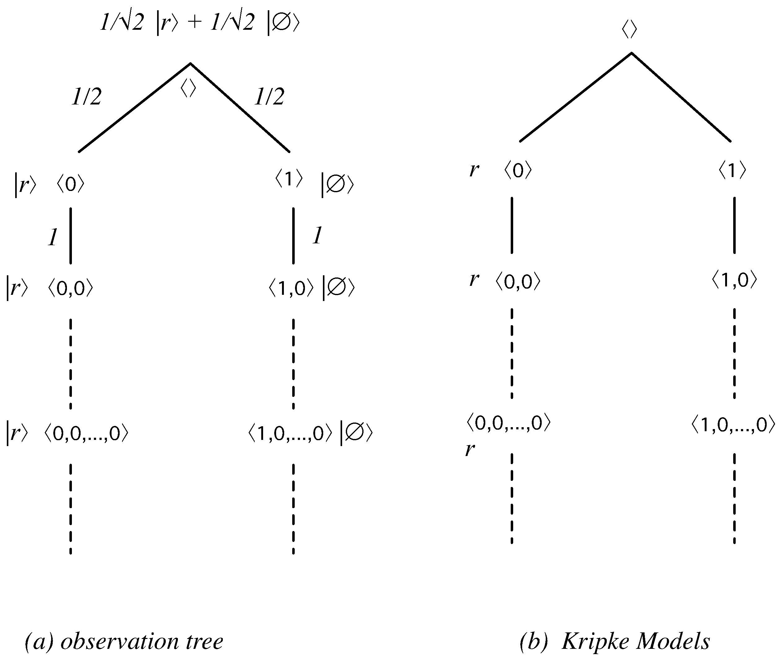
2.2. Observation Trees

We can now introduce our tree models.

Definition 3

(Observational Tree). Let $\mathbb{X}$ be a finite set of propositional symbols. An observational tree is a structure ${\mathbb{T}}_{\mathbb{X}}=\langle \langle T,\le \rangle ,\mathfrak{p},\mathfrak{a},\mathfrak{s}\rangle$ where

• $\mathcal{T}=\langle T,\le \rangle$ is an abstract tree;
• $\mathfrak{p},\mathfrak{a},\mathfrak{s}$ are the following labelling functions:

  -

  $\mathfrak{p}:\mathbb{E}\to {(0,1]}_{\mathbb{R}}$;

  -

  $\mathfrak{a}:T\to \mathfrak{M}$;

  -

  $\mathfrak{s}:T\to {\mathcal{R}}_{\mathbb{X}}\cup \{0\}$

• for which some constraints holds. Let us suppose that $\mathfrak{a}(\alpha )={(P_i)}_{i<k}\in \mathfrak{M}$, then:

  -

  $\forall i<k.(P_i(\alpha )\ne 0\Rightarrow \alpha \ast \langle i\rangle \in T)$;

  -

  if $\forall j\ge K.\alpha \ast \langle j\rangle \notin T$;

  -

  $\forall i<K$ if $\alpha \ast \langle i\rangle \in T$ then

  -

  $\mathfrak{p}(\alpha ,\alpha \ast \langle i\rangle )=〈\mathfrak{s}(\alpha )\mid P_i\mid \mathfrak{s}(\alpha )〉$

  -

  $\mathfrak{s}(\alpha \ast \langle i\rangle )=\frac{P_i(\mathfrak{s}(\alpha ))}{\sqrt{\mathfrak{p}(\alpha ,\alpha \ast \langle i\rangle )}}$

Informally:

• $\mathfrak{p}$ assigns a (correct) probability to each edge.
• $\mathfrak{a}$ assigns to each node a sequence of observations (an element in $\mathfrak{M}$), in particular the sequence that generates the current (evaluation of the) state, starting from the root node.
• $\mathfrak{s}$ assigns to each node a quantum register.

The following property trivially holds:

Proposition 1

(Monotonicity). Let ${\mathbb{T}}_{\mathbb{X}}=\langle \langle T,\le \rangle ,\mathfrak{p},\mathfrak{a},\mathfrak{s}\rangle$ be an observational tree, then

$$\forall \alpha \in T.(q\in \mathfrak{s}(\alpha )\Rightarrow \forall \beta \le \alpha .q\in \mathfrak{s}(\beta ))$$

Remark 1.

In the graphical representation of observation trees, we omit nodes labeled with 0-vectors.

3. The Logic of Observations

In this section, we semantically define the logic ${\mathcal{L}}_{\mathbb{P}}$ of quantum observations. As anticipated in the Introduction, we fix the set of propositional symbols to the set of qubit names and we adopt the standard connectives of propositional logic. Formally:

Definition 4

(Language of ${\mathfrak{L}}_{\mathbb{P}}$). The language ${\mathfrak{L}}_{\mathbb{P}}$ of ${\mathcal{L}}_{\mathbb{P}}$ is built upon propositional symbols, which we set to $\mathbb{P}$ and connectives $\to ,\wedge ,\vee ,\perp$.

We also exploit some auxiliary notation. Let us denote with ${\mathfrak{Form}}_{\mathbb{P}}$ the set of resulting well formed formulas built in the standard way. Given a formula A let we denote with $\mathbb{P}[A]$ the set of propositional symbols occurring in A.

We define now the semantics of a formula with respect to an observational tree.

Definition 5

(Semantics). The semantics of a formula A with respect to to an observational tree ${\mathbb{T}}_{\mathbb{X}}$ with $\mathbb{X}\supseteq \mathbb{P}[A]$ is defined as:

• ${\mathbb{T}}_{\mathbb{X}},\alpha ⊫q$ iff $q\in \mathfrak{s}(\alpha )$;
• ${\mathbb{T}}_{\mathbb{X}},\alpha {⊯}_{}\perp$
• ${\mathbb{T}}_{\mathbb{X}},\alpha ⊫A\wedge B$ iff ${\mathbb{T}}_{\mathbb{X}},\alpha ⊫A\&{\mathbb{T}}_{\mathbb{X}},\alpha ⊫B$
• ${\mathbb{T}}_{\mathbb{X}},\alpha ⊫A\vee B$ iff ${\mathbb{T}}_{\mathbb{X}},\alpha ⊫A\mathsf{OR}{\mathbb{T}}_{\mathbb{X}},\alpha ⊫B$
• ${\mathbb{T}}_{\mathbb{X}},\alpha ⊫A\to B$ iff $\forall \beta \le \alpha {\mathbb{T}}_{\mathbb{X}},\beta ⊫A\Rightarrow {\mathbb{T}}_{\mathbb{X}},\beta ⊫B$

Proposition 2.

1. 

${\mathbb{T}}_{\mathbb{X}},\alpha ⊫A\iff \forall \beta \le \alpha \Rightarrow {\mathbb{T}}_{\mathbb{X}},\beta ⊫A$;

2. 

${\mathbb{T}}_{\mathbb{X}},\langle \rangle ⊫A\iff \forall \alpha \in T_{\mathbb{X}}.{\mathbb{T}}_{\mathbb{X}},\alpha ⊫A$.

Proof. 

By easy induction on the structure of the formula A, following Definition 5. Let us show some case for (1), as a title of example. Let A be a propositional symbol q: the thesis follows by Proposition 1 (monotonicity). Let A be of the sharp $B\wedge C$. By i.h., for all $\beta \le \alpha$, we have both ${\mathbb{T}}_{\mathbb{X}},\beta ⊫B$ and ${\mathbb{T}}_{\mathbb{X}},\beta ⊫C$ then, by Definition 5, ${\mathbb{T}}_{\mathbb{X}},\beta ⊫B\wedge C$. Other cases are similar and (2) plainly follows from (1).  □

With ${\mathbb{T}}_{\mathbb{X}}⊫A$ we mean that $\forall \alpha .{\mathbb{T}}_{\mathbb{X}},\alpha ⊫A$ (A is true in ${\mathbb{T}}_{\mathbb{X}}$). With $⊫A$ we mean that $\forall {\mathbb{T}}_{\mathbb{P}[A]}.{\mathbb{T}}_{\mathbb{P}[A]}⊫A$ (A is valid).

It is easy to observe that, given a formula A, the set of propositional symbols is enough to state its satisfiability in a model.

Proposition 3.

Let A be a formula, then for each $\mathbb{X}\supseteq \mathbb{P}[A]$ we have that ${\mathbb{T}}_{\mathbb{X}}⊫A$ iff ${\mathbb{T}}_{\mathbb{P}[A]}⊫A$.

We can formally state a relationship between observational trees and Kripke models. In Section 3.1, we show how to extract a Kripke model from an observation tree. The converse is shown in Section 3.2.

3.1. From Observational Trees to Kripke Models

Let ${\mathbb{T}}_{\mathbb{X}}=\langle \langle T,\le \rangle ,\mathfrak{p},\mathfrak{a},\mathfrak{s}\rangle$ be an observational tree. We associate to ${\mathbb{T}}_{\mathbb{X}}$ a Kripke model ${\mathfrak{K}}_{{\mathbb{T}}_{\mathbb{X}}}=\langle T_{\mathbb{T}},{⊑}_{\mathbb{T}},V_{\mathbb{T}}\rangle$ defined in the following way:

• $T_{\mathbb{T}}=T$;
• $\alpha ⊑\beta \iff \beta \le \alpha$;
• $V_{\mathbb{T}}:T_{\mathbb{T}}\to 2^{\mathbb{P}}$ is s.t. $q\in V_{\mathbb{T}}(\alpha )\iff q\in \mathfrak{s}(\alpha )$.

Proposition 1 ensures that ${\mathfrak{K}}_{{\mathbb{T}}_{\mathbb{X}}}$ is an intuitionistic model:

Proposition 4.

${\mathfrak{K}}_{{\mathbb{T}}_{\mathbb{X}}}$ is an intuitionistic Kripke model.

The semantics interpretation the Kripke models above defined is standard:

Definition 6

(Kripke Semantics). The semantics of a formula A with respect to to an Kripke Model ${\mathfrak{K}}_{{\mathbb{T}}_{\mathbb{X}}}$ with $\mathbb{X}\supseteq \mathbb{P}[A]$ is defined as:

• ${\mathfrak{K}}_{{\mathbb{T}}_{\mathbb{X}}},\alpha ⊩q$ iff $q\in V_{\mathbb{T}}(\alpha )$;
• ${\mathfrak{K}}_{{\mathbb{T}}_{\mathbb{X}}},\alpha \neg ⊩\perp$;
• ${\mathfrak{K}}_{{\mathbb{T}}_{\mathbb{X}}},\alpha ⊩A\wedge B$ iff ${\mathfrak{K}}_{{\mathbb{T}}_{\mathbb{X}}},\alpha ⊩A\&T_{\mathbb{T}},\alpha ⊩B$;
• ${\mathfrak{K}}_{{\mathbb{T}}_{\mathbb{X}}},\alpha ⊩A\vee B$ iff ${\mathfrak{K}}_{{\mathbb{T}}_{\mathbb{X}}},\alpha ⊩A\mathsf{OR}{\mathfrak{K}}_{{\mathbb{T}}_{\mathbb{X}}},\alpha ⊩B$;
• ${\mathfrak{K}}_{{\mathbb{T}}_{\mathbb{X}}},\alpha ⊩A\to B$ iff $\forall \beta ,\alpha {⊑}_{\mathbb{T}}\beta \Rightarrow ({\mathfrak{K}}_{{\mathbb{T}}_{\mathbb{X}}},\beta ⊩A\Rightarrow {\mathfrak{K}}_{{\mathbb{T}}_{\mathbb{X}}},\beta ⊩B)$.

With ${\mathfrak{K}}_{{\mathbb{T}}_{\mathbb{X}}}⊩A$ we mean that $\forall \alpha .{\mathfrak{K}}_{{\mathbb{T}}_{\mathbb{X}}},\alpha ⊩A$ (A is true in ${\mathfrak{K}}_{{\mathbb{T}}_{\mathbb{X}}}$). With $⊩A$ we mean that $\forall {\mathbb{T}}_{\mathbb{P}[A]}{\mathfrak{K}}_{{\mathbb{T}}_{\mathbb{P}[A]}}⊩A$ (A is valid).

Moreover, the following proposition holds:

Proposition 5.

For each formula A, $\mathbb{X}\supseteq \mathbb{P}[A]$ and observational model ${\mathbb{T}}_{\mathbb{X}}=\langle \langle T,\le \rangle ,\mathfrak{p},\mathfrak{a},\mathfrak{s}\rangle$ and for each $\alpha \in T$

$${\mathbb{T}}_{\mathbb{X}},\alpha ⊫A\iff {\mathfrak{K}}_{\mathbb{T}},\alpha ⊩A$$

Proof. 

The thesis follows by construction of of the model ${\mathfrak{K}}_{\mathbb{T}}$ from the observational tree. If A is a propositional symbol q, then ${\mathbb{T}}_{\mathbb{X}},\alpha ⊫q$ iff (by definition of the semantics) $q\in \mathfrak{s}(\alpha )$, iff and only if $q\in V_{\mathbb{T}}(\alpha )$. The other cases are easily provable by induction on the structure of A. We show the ∧ case as a title of example. Suppose ${\mathbb{T}}_{\mathbb{X}},\alpha ⊫B\wedge C$. This holds iff ${\mathbb{T}}_{\mathbb{X}},\alpha ⊫B\&{\mathbb{T}}_{\mathbb{X}},\alpha ⊫C$. By i.h., we have ${\mathfrak{K}}_{\mathbb{T}},\alpha ⊩B$, ${\mathfrak{K}}_{\mathbb{T}},\alpha ⊩C$ and, by Definition 6, ${\mathfrak{K}}_{\mathbb{T}},\alpha ⊩B\wedge C$.  □

Since for each ${\mathbb{T}}_{\mathbb{X}}$, ${\mathfrak{K}}_{{\mathbb{T}}_{\mathbb{X}}}$ is a Kripke model, we have trivially that:

Corollary 1.

$⊩A\Rightarrow ⊫A$.

Corollary 1 shows that ⊫ is a logic that leaves between intuitionistic and classical logic, namely the following set of inclusions hold (⊧ is the classic logic notion of truth):

$$\{A:⊩A\}\subseteq \{A:⊫A\}⊊\{A:\vDash A\}$$

The last inclusion is trivially shown, since we known that classical validity may be formulated with finite models. A finite model is nothing else that a finite set $X\subseteq \mathbb{P}$, with the clause for propositional symbols $X\vDash q\iff q\in X$. Given a finite model $X=\{r_0,\dots ,r_n\}$, we can associate to X the observation tree $\mathbb{T}$ where the root is labelled with $\left|X\right.〉$ and for each node t, $\mathfrak{a}(t)=\{I\}$. It is trivial to observe that $X\vDash A\iff \mathbb{T}⊫A$. The thesis follows immediately.

On the other hand, as shown below, ⊫ does not validate the tertium non datur principle, and consequently the last inclusion is proper.

Theorem 1.

$⊯A\vee \neg A$

Proof. 

Let us consider the observational tree $\mathbb{T}$ represented in Figure 1. Let $\mathfrak{a}\langle \rangle =(P_r,P_r^{\perp })$ where P is the projector in the subspace of vectors $\beta$ s.t. $r\in \beta$. Moreover, for each $\alpha \ne \langle \rangle$, let $\mathfrak{a}(\alpha )=Id$. It is immediate to observe that $\mathbb{T}⊯r\vee \neg r$, and therefore $⊯r\vee \neg r$.  □

The question is now to classify ⊫ with respect to intuitionistic logic. In the next section, we show how any (tree-like) Kripke model can be translated into an observational tree.

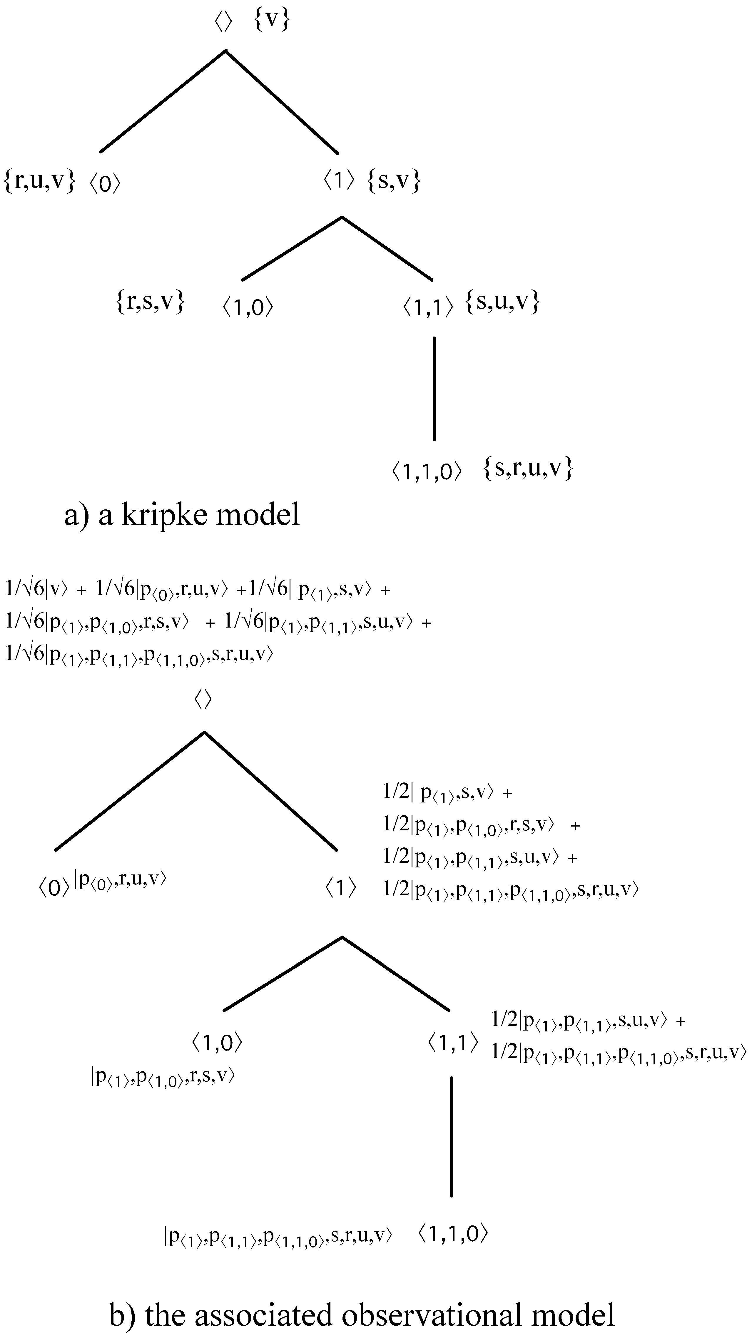
3.2. From Kripke Models to Observational Trees

We now show how to associate to a tree-Kripke model K an observational model ${\mathbb{T}}_K$.

Let K be a tree Kripke model $\langle N,\le ,V\rangle$. We denote with ${\mathbb{P}}_K$ the set of propositional symbols ${\bigcup }_{t\in N}V(t)$ and with $F_K$ the set of formulas built on the basis of ${\mathbb{P}}_K$.

Theorem 2.

For each tree-like Kripke model K and for each $A\in F_K$

$$K,t⊩A\iff {\mathbb{T}}_K,t⊫A$$

Proof. 

We show a simple procedure to associate an observational tree ${\mathbb{T}}_K=\langle N,⊑,\mathfrak{p},\mathfrak{a},\mathfrak{s}\rangle$ to $K=\langle N,\le ,V\rangle$.

Step 1

Choose a set of distinguishable propositional symbols $PN=\{p_t:t\in N\}$ s.t. ${\mathbb{P}}_T\cap N=\varnothing$ and build the Hilbert Space is ${\mathcal{H}}_{PN\cup {\mathbb{P}}_T}$.

Step 2

Define ⊑ as ${\le }^{-}1$ ($t⊑u\iff u\le t$).

Step 3

Let $\mathfrak{a}(t)$ be the set of projectors ${\mathcal{O}}_t=\{P_{i_1},\dots P_{i_m}\}$ defined as:

$${\mathcal{O}}_t=\left\{\begin{array}{c}\varnothing \mathrm{if}t\mathrm{is} \mathrm{a} \mathrm{leaf}\hfill \\ \{P_{i_1},\dots P_{i_m}\}\mathrm{s}.\mathrm{t}.\forall j\in [1,m].P_{i_j}\mathrm{is} \mathrm{the} \mathrm{projector} \mathrm{in} \mathrm{the} \mathrm{subspace} \mathrm{of} \mathrm{registers}\hfill \\ \beta \mathrm{s}.\mathrm{t}.t\ast \langle i_j\rangle \in \beta \mathrm{and}t\ast \langle i_j\rangle ⊑t,\mathrm{otherwise}.\hfill \end{array}\right.$$

Step 4

The functions $\mathfrak{p},\mathfrak{s}$ are univocally defined by the following labeling $\mathfrak{s}\langle \rangle$ of the root.

Let us consider the set of L of leaves of K, and consider for each $u\in :$ the set $C_u=\{t:t\in N\&u⊑t\&t\in N\}$ and the set $P{r}_u={\bigcup }_{t\in C_u}V(t)$. We define $\mathfrak{s}\langle \rangle ={\sum }_{u\in L}\frac{1}{\sqrt{\left|L\right|}}\left|C_u\cup P{r}_u\right.〉$

Given the above translation, the proof proceeds by means of a standard induction on the length of formulas.  □

Example 1.

Let us consider the tree-like Kripke model in Figure 2a. Applying the four steps above scripted, we obtain an observational model as in Figure 2b where the relevant Hilbert space is

$${\mathcal{H}}_{r,s,u,v,p_{\langle 0\rangle },p_{\langle 0\rangle },p_{\langle 1,0\rangle },p_{\langle 1,1\rangle },p_{\langle 1,1,0\rangle }}$$

(for the sake of readability, we have depicted only the labelling function $\mathfrak{a}$.)

As a corollary of Theorem 2, we can state the following:

Corollary 2.

$⊫A\Rightarrow ⊩A$

Therefore, Corollaries 1 and 2 give us the final theorem:

Theorem 3.

The class of valid formulas with respect to the classes of observational trees is exactly the class of intuitionistic provable formula, or in other words:

$$⊫A\iff ⊩A$$

4. Possible Developments

The further investigations based on the proposed approach will follow two different directions of research.

• We have shown that intuitionistic logic is “the” logic of observational tree. This means that we could think to move from the model theoretic approach to a proof theoretical one. It is well known that, via the so called Curry–Howard isomorphism, it is possible to associate a lambda calculus to the intuitionistic proofs. Is it possible to give a quantum interpretation of such a calculus? Our idea is to start again with the BHK interpretation of intuitionistic logic. For example, according to this interpretation, a proof of $A\to B$ could be seen as a measurement process that transforms each measurement process A into one of B.
• We think also to extend the model theoretic approach in order to deal with unitary transformations. One possibility we have in mind is to add a temporal (possibly classical or intuitionistic) dimension to intuitionistic logic, so that we can move in two different directions: an intuitionist one linked to the measurement process, and an linear temporal one that is linked to unitary evolution of the quantum system. The studies of Finger and Gabbay on the temporalization of logical system could help (see, e.g., [19].)

References

1. Birkhoff, G.; von Neumann, J. The logic of quantum mechanics. Ann. Math. 1936, 37, 823–843. [Google Scholar] [CrossRef]
2. Dalla Chiara, M.L. Quantum Logic. In Handbook of Philosophical Logic: Volume III: Alternatives to Classical Logic; Gabbay, D., Guenthner, F., Eds.; Springer: Heidelberg, Germany, 1986; pp. 427–469. [Google Scholar]
3. Feynman, R.P. Simulating physics with computers. Internat. J. Theoret. Phys. 1981/82, 21, 467–488. [Google Scholar] [CrossRef]
4. Nielsen, M.A.; Chuang, I.L. Quantum Computation and Quantum Information, 10th Anniversary ed.; Cambridge University Press: Cambridge, UK, 2010; p. xxvi+676. [Google Scholar]
5. Selinger, P.; Valiron, B. A lambda calculus for quantum computation with classical control. Math. Struct. Comput. Sci. 2006, 16, 527–552. [Google Scholar] [CrossRef]
6. Díaz-Caro, A.; Arrighi, P.; Gadella, M.; Grattage, J. Measurements and Confluence in Quantum Lambda Calculi With Explicit Qubits. Electr. Notes Theor. Comput. Sci. 2011, 270, 59–74. [Google Scholar] [CrossRef] [Green Version]
7. Pagani, M.; Selinger, P.; Valiron, B. Applying quantitative semantics to higher-order quantum computing. In Proceedings of the POPL’14, San Diego, CA, USA, 22–24 January 2014; ACM: New York, NY, USA, 2014; pp. 647–658. [Google Scholar] [Green Version]
8. Zorzi, M. On quantum lambda calculi: A foundational perspective. Math. Struct. Comput. Sci. 2016, 26, 1107–1195. [Google Scholar] [CrossRef]
9. Coecke, B.; Duncan, R. Tutorial: Graphical Calculus for Quantum Circuits; Reversible Computation; Glück, R., Yokoyama, T., Eds.; Springer Berlin Heidelberg: Berlin/Heidelberg, Germany, 2013; pp. 1–13. [Google Scholar]
10. Dal Lago, U.; Zorzi, M. Wave-Style Token Machines and Quantum Lambda Calculi. In Proceedings of the Third International Workshop on Linearity (LINEARITY 2014), Vienna, Austria, 13 July 2014; Volume 176, Electronic Proceedings in Theoretical Computer Science. pp. 64–78. [Google Scholar] [CrossRef]
11. Paolini, L.; Zorzi, M. qPCF: A language for quantum circuit computations. In Proceedings of the Theory and Applications of Models of Computation—14th Annual Conference, TAMC 2017, Bern, Switzerland, 20–22 April 2017; Volume 10185, Lecture Notes in Computer Science. pp. 455–469. [Google Scholar] [CrossRef]
12. Abramsky, S.; duncan, R. A categorical quantum logic. Math. Struct. Comput. Sci. 2006, 16, 469–489. [Google Scholar] [CrossRef]
13. Baltag, A.; Smets, S. Quantum logic as a dynamic logic. Synthese 2011, 179, 285–306. [Google Scholar] [CrossRef]
14. Baltag, A.; Smets, S. LQP: the dynamic logic of quantum information. Math. Struct. Comput. Sci. 2006, 16, 491–525. [Google Scholar] [CrossRef]
15. Masini, A.; Viganò, L.; Zorzi, M. Modal deduction systems for quantum state transformations. J. Mult.-Valued Logic Soft Comput. 2011, 17, 475–519. [Google Scholar]
16. Viganò, L.; Volpe, M.; Zorzi, M. Quantum State Transformations and Branching Distributed Temporal Logic—(Invited Paper). In Proceedings of the Logic, Language, Information, and Computation—21st International Workshop (WoLLIC 2014), Valparaíso, Chile, 1–4 September 2014; Volume 8652, Lecture Notes in Computer Science. pp. 1–19. [Google Scholar] [CrossRef]
17. Viganò, L.; Volpe, M.; Zorzi, M. A branching distributed temporal logic for reasoning about entanglement-free quantum state transformations. Inf. Comput. 2017, 255, 311–333. [Google Scholar] [CrossRef] [Green Version]
18. Girard, J.Y. Proof Theory and Logical Complexity; Studies in Proof Theory. Monographs; Bibliopolis: Naples, Italy, 1987; Volume 1, p. 505. [Google Scholar]
19. Finger, M.; Gabbay, D. Combining Temporal Logic Systems. Notre Dame J. Formal Logic 1996, 37, 204–232. [Google Scholar] [CrossRef]
Figure 1. Tertium non datur: a counterexample.
Axioms 08 00025 g001
Figure 2. The transformation of a Kripke model in a observational tree.
Axioms 08 00025 g002