Article

A New Generalized Projection and Its Application to Acceleration of Audio Declipping

1
Signal Processing Laboratory, Brno University of Technology, 616 00 Brno, Czech Republic
2
Faculty of Mechanical Engineering, Brno University of Technology, 616 69 Brno, Czech Republic
*
Author to whom correspondence should be addressed.
Current address: Technická 12, 616 00 Brno, Czech Republic.
Axioms 2019, 8(3), 105; https://doi.org/10.3390/axioms8030105
Submission received: 6 March 2019 / Revised: 9 September 2019 / Accepted: 10 September 2019 / Published: 19 September 2019
(This article belongs to the Special Issue Harmonic Analysis and Applications)

Abstract

:
In convex optimization, it is often inevitable to work with projectors onto convex sets composed with a linear operator. Such a need arises from both the theory and applications, with signal processing being a prominent and broad field where convex optimization has been used recently. In this article, a novel projector is presented, which generalizes previous results in that it admits to work with a broader family of linear transforms when compared with the state of the art but, on the other hand, it is limited to box-type convex sets in the transformed domain. The new projector is described by an explicit formula, which makes it simple to implement and requires a low computational cost. The projector is interpreted within the framework of the so-called proximal splitting theory. The convenience of the new projector is demonstrated on an example from signal processing, where it was possible to speed up the convergence of a signal declipping algorithm by a factor of more than two.

1. Introduction

Proximal algorithms are a modern branch of mathematical optimization, whose principal building blocks are the so-called proximal operators [1,2,3,4]. In applications, the model of the problem often involves the composition of a non-linear function with a linear operator [5,6,7,8,9,10]. When proximal optimization is utilized to find approximate solution iteratively, the proximal operator of such a composition is needed, making the resulting algorithms computationally expensive in general [11]. However, there are special cases in which the proximal operator can be expressed explicitly [2,12,13,14].
In the paper, we introduce and prove a new lemma which provides an explicit formula for the evaluation of the projector onto a convex set, composed with a linear operator. It is motivated by an already known property of proximal operators of functions composed with semi-orthogonal linear operators [2]. Actually, our lemma generalizes the previous result in two directions, since it admits working in a complex vector space and the linear operator is only assumed to satisfy a certain diagonality property. On the other hand, the new projection formula is limited to projectors onto box-type sets. Since projectors represent a special case of proximal operators, our lemma falls into the general concept of proximal minimization; nevertheless, our result is valuable per se, since projections are used in many other contexts and fields of science.
As an example, we apply the novel projection to the problem of signal declipping, i.e., to the restoration of unknown parts of a signal degraded by clipping/saturation, which is a non-linear distortion of an audio signal, described in detail in the experimental part. The declipping model is quite simple, since it is not the goal of this paper to develop a method that outperforms the state of the art, but rather to illustrate the use of the proposed lemma in a technical application arising from the field of audio signal recovery.
In Section 2, the proximal and projection operators are reviewed and the state of the art in this specific area is presented. Next, the novel generalized projection is introduced, including the proof. Section 3 then discusses the result and emphasizes its advantages over the current methods, and also points out its limitations. Based on the new result, an example experiment in the signal processing field is presented in Section 4, where we show that audio declipping benefits from our approach by the computation being accelerated by a factor of at least two.

2. Methods

2.1. Proximal Algorithms

The proximal algorithm is an iterative algorithm that, under certain conditions, provides a sequence of vectors { x k } converging to the minimizer of a sum of convex functions i f i ( x ) . This is achieved by sequential evaluation of the so-called proximal operators associated with each of the summands, f i . The most often used and studied are proximal algorithms that can minimize the sum of two convex functions, f 1 ( x ) + f 2 ( x ) , such as the Forward–backward algorithm or the Douglas–Rachford algorithm [13,15]; however, there exist algorithms for minimizing the sum of arbitrarily many functions [2].
Algorithms that can minimize a sum involving a linear operator have been presented only recently. Chambolle and Pock [5] presented a primal–dual algorithm that minimizes the sum of two functions f 1 ( x ) + f 2 ( L x ) where neither f 1 nor f 2 has to be smooth. The Forward–backward based primal—dual (FBB-PD) algorithm [6] can cope with the sum of three functions f 1 ( x ) + f 2 ( x ) + f 3 ( L x ) , where f 2 is smooth. The most general algorithm published by Condat [7,11] admits the minimization of any finite number of functions with the inclusion of potentially multiple linear operators, f 1 ( x ) + f 2 ( x ) + f 3 ( L 3 x ) + + f K ( L K x ) .

2.2. Proximal Operators

Let R ˜ denote the extended real line, i.e., R ˜ = R { , } . Proximal operators are the key components in proximal algorithms. Recall that the proximal operator of a convex function h : C N R ˜ maps z C N to another vector in C N , such that [3,16]
prox h ( z ) = arg~min x C N h ( x ) + 1 2 z x 2 2 .
The proximal operator is a generalization of a projection operator onto a convex set—this fact is clear if we identify h with the indicator function ι K of such a set K; in such a case [1],
h ( x ) = ι K ( x ) = 0 for x K for x K ,
and we get the relation proj K = prox ι K . For a convex h, the map in Equation (1) is uniquely defined [2]. A characterization of proximal operators of convex lower semicontinuous functions is the work of Moreau [16].
In this article, we are interested in the proximal operator of the map f ( L · ) = f L . Let us denote such a composition h ( x ) = ( f L ) ( x ) = f ( L x ) , with L : C N C M . If f is convex, then f L is also convex, which is straightforward to show. Therefore, in line with Equation (1), our goal is to find
prox f L ( z ) = arg~min x R N f ( L x ) + 1 2 z x 2 2 .
Although explicit formulas exist for many particular choices of h in Equation (1) (see, e.g., [2]), the situation gets complicated for the compositions in Equation (2). In addition, note, that when prox h is available, then prox ν h is often easy to find for ν > 0 .
In many practical situations, one can benefit from the following lemma, occurring, for example, in ([2], Table 10.1.x). Let Id denote the identity operator, i.e., Id ( x ) = x ; the optional subscript indicates the dimensionality of x .
Lemma 1.
Let L be a linear operator, L : R N R M , such that L L = ν Id M , ν > 0 . Then,
prox f L = Id N + ν 1 L ( prox ν f Id M ) L .
L denotes the adjoint of L; the symbol is used here to emphasize that L is assumed to be real. In the finite-dimensional case, L can be understood as the transpose of the M × N matrix identified with L. The property described by the above lemma can be found in [3,12,13,14], exhibiting different styles of proof but limited to real space setting. Equation (3) says that, to evaluate the composite proximal operator, it is sufficient to know the proximal operator of ν f and to be able to perform L and L . For an arbitrary z R N , this means
prox f L ( z ) = z + ν 1 L ( prox ν f ( L z ) L z ) .
The assumption L L = ν Id is called “semi-orthogonality” of L in [2]; from the viewpoint of frame theory, such an L corresponds to a synthesis operator of a so-called tight frame with the frame constant ν [17,18,19,20,21]. Note that as a consequence of the assumption, it automatically holds M N due to M = rank ( L L ) = rank ( L ) N . Equation (3) drastically reduces the complexity of computations when prox f is known, since Equation (2) is then solved explicitly when compared with the general case.
Note that a tight frame synthesis operator L acts the same way as an orthonormal operator does, since both satisfy L L = ν Id ( ν = 1 in both the orthonormal case and the case of Parseval tight frame [17]). Expressed in words, the analysis followed by the synthesis reproduces the object. Observe that the opposite L L = ν Id is true if and only if L is orthonormal (unitary) operator R N R N as a special case of Parseval tight frame with ν = 1 and M = N .
Example 1.
As an example, the projection onto the set { z | L z y 2 δ } has to be computed iteratively in general; however, when L is a synthesis operator of a tight frame, such a projection can be evaluated explicitly by
proj { z | L z y 2 δ } ( x ) = x + ν 1 L proj { z | z y 2 δ } ( L x ) L x ,
i.e., using a simple projection onto the ball { z | z y 2 δ } . Note that the set { z | L z y 2 δ } represents an ellipsoid in R N when bijective L : R N R N is considered.
At this point, we recall the pseudoinverse operator, which is used in the rest of the paper. Lemmas 2 and 3 are discussed, for example, in ([22], Section 5.13).
Lemma 2.
Let L : C N C M , M N be a surjective linear operator and y R M . Then, L + y is the least-norm solution to the system L x = y , i.e., L + y 2 x 2 , for any x satisfying L x = y . The pseudoinverse operator L + is in this surjective case defined through L + = L * ( L L * ) 1 .
The application of L + L corresponds to projecting onto the range space of L . Another, more common case of projection is the projection onto an affine subspace. The motivation for the related following lemma is twofold: First, the described projection belongs to the “family” of proximal operators we are concerned with. Second, this result is utilized below in the experiment. To put it into context, this lemma holds for any complex b , but, on the other hand, its application is limited to affine spaces only.
Lemma 3.
Let L : C N C M be any surjective linear operator and b C M . Then, the projection of a vector z C N onto the affine space Γ = { u C N | L u = b } can be expressed as
proj Γ ( z ) = z + L + b L z .
Proof. 
The proof is based upon the observation that the affine subspace Γ is parallel to the subspace { u C N | L u = 0 } , which is the kernel of the operator L. We thus use the projection of z onto the kernel of L, which is ( z L + L z ) . The demanded projection onto Γ is then obtained by the shift between Γ and the kernel of L, which is L + b , leading to
proj Γ ( z ) = ( z L + L z ) + L + b ,
which equals Equation (6) after rearranging. □
Under the assumption of Lemma 1, the relation in Equation (6) is a special case of Equation (4) in view of L + = ν 1 L with f set to the indicator function of set { b } consisting of this single point. Then, Equation (6) belongs to the family of proximal operators. Without these assumptions, we get a different type of projection. Relaxing the assumptions on L L * (where L * denotes the Hermitian transpose or adjoint operator of L) to be an arbitrary diagonal matrix allows us to replace the one-point set by a more general box-type set as shown in the next subsection.

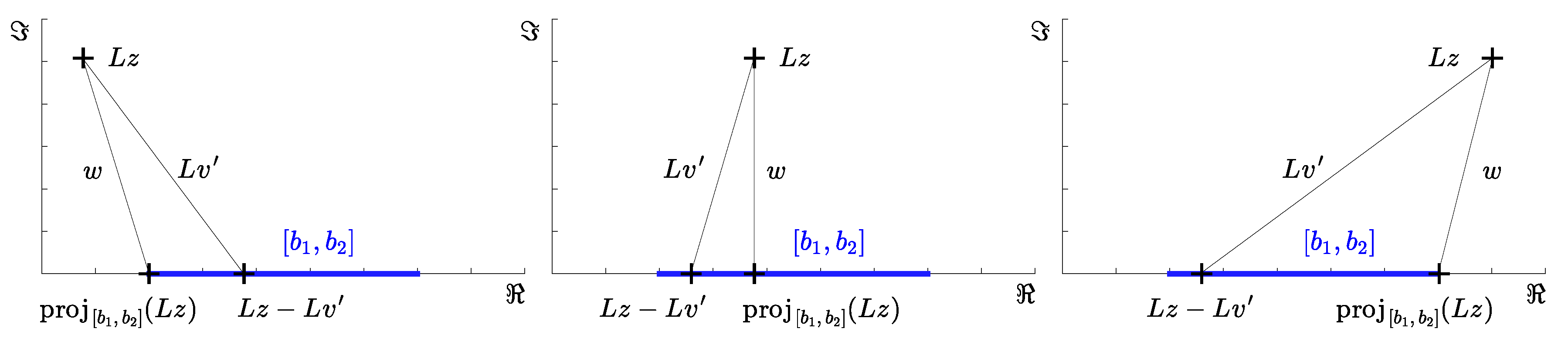
2.3. The New Relation of Projections

First, two concepts known from matrix algebra are adopted. We do this to emphasize that our result could be generalized to an infinite-dimensional (both countable and uncountable) setting, although below we reside in finite-dimensional spaces, where a linear operator uniquely coincides with a matrix. Expansions in separable infinite-dimensional spaces should be interpreted “in norm”, e.g., the notation x = k x k e k means lim n x k n x k e k 0 .
Definition 1.
A linear operator D defined on a Hilbert space X is calleddiagonal with respect to a basis { e k } k N if it holds
D e k = λ k e k for all k N ,
where λ k are complex scalars. In the finite-dimensional complex space, by calling an operator simply diagonal we mean diagonal with respect to the canonical (standard) basis, i.e., to the set [ 1 , 0 , , 0 ] , , [ 0 , , 0 , 1 ] .
The same way as a diagonal matrix does, a bounded diagonal operator performs entry-wise, since X x = k x k e k and thus D x = k x k D e k = k ( λ k x k ) e k .
Lemma 4 (the new lemma).
Let L : C N C M be a surjective linear operator with M N and let L L * be a diagonal operator. Assume multidimensional interval bounds b 1 , b 2 R ˜ M such that b 1 b 2 , with the inequality being interpreted element-wise. Then, the projection of a vector z C N ,
proj Γ ( z ) = arg~min u Γ z u 2 ,
where Γ = { u C N | ( L u ) [ b 1 , b 2 ] , ( L u ) = 0 } ,
can be evaluated as
proj Γ ( z ) = z + L + proj [ b 1 , b 2 ] ( L z ) L z ,
where
proj [ b 1 , b 2 ] ( y ) = min max ( b 1 , ( y ) ) , b 2 , y C M .
Here, Equation (11) is the projection of the complex vector y onto a real multidimensional interval [ b 1 , b 2 ] R ˜ M with min and max functions returning pairwise extremes entry-by-entry.
The proposed lemma says that a projection (following a linear transform L) onto the box-type set Γ can be made simpler and faster using projection onto the interval [ b 1 , b 2 ] , which does not involve L. In Equation (10), the application of L + reduces to entrywise multiplication by the inverse diagonal of L L * followed by L * (see Lemma 2). Therefore, the cost of L + will typically be in the order of the cost of L * .
Before we prove the main Lemma 4, we present several auxiliary lemmas needed below.
Lemma 5.
Let L : C N C M , M N be a surjective operator, and L L * diagonal with respect to a certain basis. Then, ( L + ) * L + is diagonal with respect to the same basis.
Proof. 
The operator L is surjective and therefore its pseudoinverse can be computed as in Lemma 2. Then,
( L + ) * L + = ( L L * ) 1 * L L * ( L L * ) 1 = ( L L * ) 1 * = ( L L * ) 1 ,
which is the inverse of the diagonal operator L L * , and thus it is diagonal as well. □
Lemma 6.
Given any linear operator L : C N C M and vector y C N , the vector L + L y C N is the vector of minimal norm that is mapped by L to L y .
Proof. 
Consider the linear system L x = L y with y fixed. Using the properties of the pseudoinverse (Lemma 2), the minimum-norm solution to such a system is found by pseudoinverting the right hand side, i.e., by L + ( L y ) . □
Lemma 7.
Let W : C M C N be such an operator that W * W is diagonal with respect to a given orthonormal basis { e n } and let x , y C M . Then, from | x m | | y m | m , where x m , y m are the vector coordinates with respect to the same orthonormal basis { e n } , it follows that W x 2 W y 2 .
Proof. 
Since W * W is a diagonal operator with respect to { e n } , according to Definition 1, we have W * W e m = λ m e m for a set of scalars { λ m } , which in this case are real and nonnegative thanks to the positive semidefiniteness of W * W . Now, W x 2 2 = W x , W x = W * W x , x using the basic property of the adjoint operator. Thus, for x = m x m e m , it holds that
W x 2 2 = W * W m x m e m , m x m e m = m x m W * W e m , m x m e m = m x m λ m e m , m x m e m = m λ m | x m | 2 ,
where in the last equality we have used the linearity of the inner product and the orthonormality of { e m } . If | x m | | y m | , then also their squares satisfy | x m | 2 | y m | 2 for each m and therefore W x 2 2 = m λ m | x m | 2 m λ m | y m | 2 = W y 2 2 , since all λ m are nonnegative. □
Observe that W * W is symmetric and nonnegatively definite and thus always diagonalizable in the eigenvector orthonormal basis using the spectral theorem. Unfortunately, in applications of Lemma 4, the problem statement is typically not invariant with respect to unitary transforms (see the declipping problem in Section 4). Thus, we have to keep to the standard basis when expanding the projected vector in most cases.
Proof of Lemma 4.
First, we show that Equation (11) is indeed a projector onto [ b 1 , b 2 ] . Since the set [ b 1 , b 2 ] is a multidimensional box (possibly open towards plus or minus infinity), the projection proj [ b 1 , b 2 ] ( y ) can be evaluated entry-by-entry. Fix m and consider the mth entry y m = : y , ( b 1 ) m = : b 1 , ( b 2 ) m = : b 2 . In accordance with the definition of projection,
proj [ b 1 , b 2 ] ( y ) = arg~min b 1 x b 2 | x y | = arg~min b 1 x b 2 ( x ( y ) ) 2 + ( y ) 2 = arg~min b 1 x b 2 ( x ( y ) ) 2 + ( y ) 2 = arg~min b 1 x b 2 | x ( y ) | ,
i.e., the original task reduces to projecting ( y ) onto [ b 1 , b 2 ] . We prove Equation (11) by evaluating the only three possibilities (for a single entry but applied to all of them):
proj [ b 1 , b 2 ] ( y ) = min ( max ( b 1 , ( y ) ) , b 2 ) = b 1 for ( y ) < b 1 , b 2 for ( y ) > b 2 , y for b 1 ( y ) b 2 .
Now, return back to Equation (10). Suppose that z Γ ; then, ( L z ) [ b 1 , b 2 ] ; from Equation (11), we have proj [ b 1 , b 2 ] ( L z ) = L z ; and, from Equation (10), we get proj Γ ( z ) = z , which is correct. In the complementary case, z Γ and due to L being surjective, there exists at least one v C N for which
L v = L z proj [ b 1 , b 2 ] ( L z ) = : w .
Trivially, any such vector v satisfies L ( z v ) = proj [ b 1 , b 2 ] ( L z ) [ b 1 , b 2 ] , i.e., z v Γ . In line with Equation (9a), we are looking for the shortest v , which is found using the pseudoinverse:
v + : = L + w .
Let us pick another vector v C N such that ( z v ) Γ , i.e., L ( z v ) [ b 1 , b 2 ] . We show that v 2 v + 2 . The projection in Equation (11) is performed entrywise and thus it must hold that
| w m | | ( L v ) m | for m = 1 , , M .
Figure 1 shows an illustration.
From Lemma 5, it follows that ( L + ) * L + is diagonal. Hence, we have by Lemma 7
v + 2 = L + w 2 L + ( L v ) 2 .
Finally, Lemma 6 states that L + ( L v ) 2 v 2 , which together with Equation (19) concludes the proof. □

3. Discussion on the New Result

Our Lemma 4 allows us to cover a broader scope of operators than Lemma 1 does. Specifically, L can be an arbitrary complex operator, and, moreover, L L * can be a diagonal operator, not just a multiple of the identity. On the other hand, the generalized relation only holds for a projector onto a box-type set and not for a generic proximal operator.
Example 1 shows that projecting onto an ellipsoid could be performed quickly in the special case of L L * = ν Id . In the case of the diagonal L L * , this is no longer possible.
Remark 1.
Lemma 4 clearly holds when L is the synthesis operator of a tight frame (in such a case, L L * = ν Id is a multiple of the identity). The property is still valid when such a synthesis operator is weighted column-by-column by a diagonal operator D, which is real and positive. This concept actually corresponds to the so-called weighted frames [23,24,25]. Substituting D L for L still meets the assumptions of the theorem, since ( D L ) ( D L ) * = D L L * D * = ν D D * , which is again diagonal. Such a particular setup is referred to as the painless non-orthogonal expansion in the literature [26].
Remark 2.
On the contrary, consider that L is an analysis operator, L : C N C M , M > N (i.e., L * is the synthesis operator). First, L L * cannot be diagonal by the same argumentation as on page 3 (while actually L * L can be diagonal). Lemma 4 cannot be formulated for such L, even if such a condition in the assumption is omitted; the problem appears early in the proof, in Equation (16). This linear system does not need to have any solution v for fixed z , and therefore by using Equation (11) we do not need to obtain a vector in Γ.
Remark 3.
It is clear that, if we choose L surjective, but not obeying that L L * is diagonal, the proof is ruined in Equation (19), since Lemmas 7 and 5 cannot be used. In such a situation, Equation (10) would provide a feasible solution to the problem in Equation (9), which would not guarantee to be the optimal one.
Remark 4.
Consider the common discrete Fourier transform (DFT) (see [17,27] or [28], Section 3.6). The related synthesis and analysis operators, L and L * , respectively, are complex and unitary. Without details, which come in Section 4.2, recall that they have such a special complex-conjugate structure that, when x is a real signal, L L * x = x is real again, while L * x bears the same complex-conjugate structure. In such a case, when the coefficient vector z is fed into Equation (10), L z is real and so is its projection proj [ b 1 , b 2 ] ( L z ) . Thus, L + is applied to a real vector. Since L L * = Id for the DFT, it follows that the pseudoinverse L + = L * = L 1 bears the structure of L * . As a consequence, the resulting projection is also complex-conjugate. Therefore, in theory, taking the real part in Equation (11) is redundant for the DFT. It is shown below that time–frequency operators used in the experiment have this feature as well.

4. Experiment

The so-called clipping is an artifact occurring in signal acquisition or processing, when the dynamic range of a signal is larger than the representation range of a device which is used to record or process the signal. In audio processing, this typically happens when an analog signal is captured with an analog-to-digital converter whose pre-amplifier is set such that the largest signal values are beyond the maximum digital representation level. Clipping is an annoying effect, and it introduces plenty of unwanted higher harmonic components to the signal [29].
The process of restoring as much audio information as possible, based on the degraded signal, is usually called declipping. Such a restoration task is clearly ill-conditioned, since there are infinitely many possible solutions to the problem. Declipping methods thus have to rely on additional information that characterizes the signal.
Besides other types of signal modeling [30,31,32,33,34], sparse priors have recently become very popular. Such a type of regularization assumes that the signal can be well approximated by only a few synthesis coefficients. As the transforms, the cosine (DCT and MDCT) [35,36] or the short-time Fourier transform (STFT) [37,38] are typically used. Since finding truly sparse solutions is NP-hard, various strategies are used to approximate the solution. Two major groups of algorithms can be identified: the greedy algorithms [39,40,41,42,43] and the convex-relaxation algorithms [37,38,44], or algorithms combining both approaches [36].
In our experiment, a convex formulation of the declipping problem was utilized with (synthesis) sparsity in the STFT (also termed Gabor) domain. It is shown that, when the Gabor frame fulfills the requirements of Lemma 4, as a consequence the projection onto the time-domain constraints can be done in a single step, leading to the use of a simple algorithm and speeding up the convergence by a factor of 2–3, compared to the situation when the projection is not used. We show the benefit of our novel projection on a simple declipping model, being aware that more sophisticated models cited above lead to a better quality of reconstruction.

4.1. Problem Formulation

It is assumed that a discrete-time signal y c R M is given that has been hard-clipped, i.e., any original time-domain sample above the clipping level θ H has been substituted by θ H and analogously for the samples below the level θ L . The rest of the samples in y c have not been altered by clipping, and they are called reliable.
It is furthermore assumed that the unknown original signal y is sparse or compressible in the STFT domain, formally written as y G c with c 0 N , where G is the linear Gabor synthesis operator [17], and where the pseudo-norm c 0 counts the non-zero elements of c . Characterizing the audio signal with such an operator G represents a suitable choice, since it is close to the kind of time-frequency analysis that takes place in the process of human perception [19,21]. The assumption of sparsity in the STFT domain is most realistic for solo instruments producing tones, for example the violin, double bass, piano, guitar, etc. [45,46] For instruments producing rich spectra as the drums or even for musical bands or orchestras, the number of components in the STFT domain increases and the recovery results get worse. This goes hand in hand with the reasoning that clipping enriches the STFT representation, while the sparsity-based declipping attempts to revert this process and get back the sparse representation.
In this paper, we utilize the 1 -norm as a convex surrogate of the sparsity pseudo-norm [47] and we formulate the optimization problem as
arg~min c c 1 subject to M R G c = M R y c ( reliable samples ) M H G c θ H ( samples clipped from above ) M L G c θ L ( samples clipped from below ) ,
where M R , M H , M L are simple projection operators (masks) selecting only samples related to the reliable and the clipped parts, respectively. To be precise, if we denote R , H , L the disjoint sets coinciding with the three conditions in Equation (20), i.e.,
R = { c | M R G c = M R y c } , H = { c | M H G c θ H } , L = { c | M L G c θ L } ,
then M R , M H , M L select from the complete set of indexes { 1 , , M } = R H L . The formulation in Equation (20) thus looks for coefficients that are approximately sparse and at the same time generate a signal that is consistent with the time-domain constraints.

4.2. The Gabor Operators

As a prelude to Gabor operators, return to the ordinary DFT. The DFT analysis, F * : C M C Q , computes scalar products of the signal with complex exponentials
1 Q exp i 2 π 0 q Q , exp i 2 π 1 q Q , , exp i 2 π ( M 1 ) q Q
for each frequency q = 0 , , Q 1 . Following Remark 4, we now recall that the DFT operator takes the real signal into the complex domain of dimension Q such that the image has a complex-conjugated structure. To make this statement precise, F * : R M K Q , where we define
K Q = c C Q | c 0 , c Q 2 R ; c q = c Q q ¯ , q = 1 , , Q 2 1 .
Such a structure follows immediately from Equation (22). In the common DFT case, Q = M , which implies that Equation (22) is an orthonormal basis of C M , and thus F * = F 1 . Nevertheless, the relation between coefficients holds true also in the case Q > M (with Q even) in Equation (22), which is referred to as the overcompleteness in frequency and sometimes as the redundant DFT. In such a situation, the complex exponentials form a Parseval tight frame of C M [17]. Both cases can be computed using the FFT.
The Gabor transform is a time-frequency transform with an extra structure of the coefficients in the time direction compared to the DFT. The Gabor analysis G * of a signal consists of windowing it and then taking scalar products of such windowed signal with complex harmonics in Equation (22); effectively, G * amounts in computing the FFTs of the windowed signals. The window moves along the signal by means of translation by a constant amount of samples (see below). Generally, G * : C M C N , N > M and the other way round for the synthesis G.
Conditions are known which guarantee that the frame operator G G * is invertible. The invertibility is a crucial property since its violation would mean that the synthesis operator G is not surjective. Under even stronger assumptions, the related synthesis operator G moreover bears the same time-frequency structure as G * does; this fact is handy both for the theory and practice, since in such a case, for example, the synthesis can be expressed using windows moving along time direction, as is the case of the analysis. For more details on this wide topic, see, for example, ([18], [Ch. 9]) or ([17], [Ch. 9 and 10]) or [19]. From the computational point of view, systems for which G G * = ν Id M are preferably used in applications (see, e.g., [21,41,48,49,50,51,52]), however let us note that the assumptions of our lemma, in addition, cover an important class of the so-called painless Gabor transforms [26], for which the operator G G * is diagonal and the diagonal is not necessarily constant. Gabor Parseval tight frames thus fall into our setup as a special case.
For the Gabor transform, parameters have to be specified such as the window shape and length, time-shift a of the window, and the number of frequency channels Q [19]. The number of time samples M must be a multiple of a [51]; then, the analysis operator is G * : R M C M Q / a . Recall now that the DFT analysis is an operator R M K Q ; thanks to the just described windowing, it is clear that we can even understand the operator as G * : R M K Q × × K Q , where each of the vectors from K Q originates in one of the M / a possible window positions. The synthesis G : K Q × × K Q R M produces a real signal again. It is made clear in Section 4.7 that computations in the algorithms do not tackle the coefficients in such a way that they would fall out of the space K Q × × K Q , making it possible to omit the real-part operator in Equation (11).

4.3. Problem Solution

We use the so-called proximal splitting algorithms to solve Equation (20). Proximal splitting algorithms are introduced in Section 2. First, it is convenient to rewrite Equation (20) to an unconstrained form using indicator functions (defined in Section 2) as
arg~min c C N c 1 + ι R ( c ) + ι H ( c ) + ι L ( c )
where the sets of indexes are defined in Equation (21). Once optimal coefficients are found, signal recovery is simply obtained by their synthesis through G. Equation (24) presents a sum of convex functions, considering the fact that the sets R , H , L are convex. Therefore, Equation (24) is suitable to be solved by a proximal algorithm.
Recall that proximal algorithms rely on evaluating the so-called proximal operators linked to the functions present in the sum. It is known that the proximal operator of λ · 1 is the soft thresholding with threshold λ > 0 [53,54,55] defined such that soft λ ( z ) takes the vector argument and performs elementwise mapping
z i sgn ( z i ) · max ( | z i | λ , 0 ) .
The proximal operator of ι K is the projection onto the convex set K [1,2], which is discussed in Section 2.2. Performing soft thresholding is a simple operation, but, regarding projections onto the sets R , H , L , it becomes more complicated. Explicit formulas for projecting onto these sets are known only for G being an unitary operator or a synthesis operator of a tight frame ( G G * = ν Id M ) defined in real domain (see Lemma 1). Our G, however, maps C N R M and moreover there are practical Gabor systems for which G G * is only diagonal [19,26].
In this experiment, we compared two approaches to overcome this complication. One is to adapt the general Condat algorithm (CA), which allows us to simplify the projections at the cost of an additional application of G and G * in each iteration. The second approach utilizes the novel projection lemma and shows its superiority over the first choice.

4.4. Condat Algorithm

The problem in Equation (24) is equivalent to
arg~min c c 1 + ι R ( c ) + ι H ( G c ) + ι L ( G c )
where H = { z | M H z θ H } and L = { z | M L z θ L } . Note that projection onto such sets is trivial compared to projections onto H and L, since H and L are time-domain sets for which the closest vector is found by simple elementwise comparison of the vector with clipping thresholds θ H and θ L , respectively. Regarding the reliable part of the signal, we could also resort to replacing ι R ( c ) by ι R ( G c ) , where projecting onto R = { z | M R z = M R y c } amounts to simple substitution of z with y c at the reliable positions. Note, however, that R is an affine set and there exists an explicit formula for the respective projection (see Lemma 3). In our setup, this lemma renders the following corollary.
Corollary 1.
Let G be a linear synthesis operator, G : C N C M such that G G * is diagonal. Let M R be the “reliable” mask operator, as discussed in Section 4.1. Then, for the projection onto R, we have
proj R ( z ) = z + G * M R ( M R G G * M R ) 1 ( M R y c M R G z ) .
Proof. 
We use Lemma 3 in the particular case of the diagonal product. The roles of L and b are played by M R G and M R y c , respectively. The only step to comment on is the determination of the pseudoinverse operator. Recall that G is assumed to be surjective; therefore, M R G spans the subspace onto which it projects, since M R is applied elementwise. Therefore, we can use the formula mentioned in Lemma 2 and obtain
( M R G ) + = ( M R G ) * ( M R G G * M R * ) 1 = G * M R ( M R G G * M R ) 1 .
Equation (27) follows immediately. □
Equation (27) employs application of one synthesis and one analysis. Note that ( M R G G * M R ) is a square diagonal matrix whose size equals the number of reliable samples, and, as such, its inversion is simple and can be precomputed.
The complete Condat algorithm for declipping is described in Algorithm 1. The sufficient condition on the step sizes τ and σ ensuring convergence of the algorithm involves norms of the linear operators L j of the function to minimize: τ σ j L j * L j 1 (see [7,11]). In our case, checking the problem in Equation (26) reveals that it involves an identity operator and twice the synthesis G, and it can be shown that our particular convergence criterion becomes τ σ Id + G * G + G * G 1 , where · is the operator norm. With the help of the inequality Id + G * G + G * G Id + G * G + G * G , we find a (suboptimal) bound for the step sizes. Since G G * is diagonal and it holds L * L = L L * for any operator, we have G * G = max diag | G G * | = : μ . Thus, τ σ 1 / ( 1 + 2 μ ) ensures convergence; for Parseval frames, it simplifies to τ σ 1 / 3 . However, the choice of particular σ and τ influences the convergence speed. Regarding ρ , which plays the role of an extrapolation parameter, setting it between 1 and 2 usually provides the fastest convergence in practice [11].
Algorithm 1: Condat algorithm (CA) adapted to solving Equation (26).
Axioms 08 00105 i001
In practice, we terminate the main loop when a proper convergence criterion is fulfilled (discussed below). Usually, when the algorithm stops, the solution might happen to lie slightly out of the feasible set. Therefore, we normally perform a final projection of the current solution onto the feasible set. (This also applies to the second algorithm below.)
The advantage of the Condat algorithm is its universality; it would work for audio declipping with arbitrary (meaningful) linear operator G. In the following, however, we exploit the special properties of G, which are assumed.

4.5. Douglas–Rachford Algorithm

Now, we approach the problem in Equation (24) directly. Notice that it could be rewritten as a sum of two convex functions
arg~min c c 1 + ι K ( c )
with K = { z | M R G z = M R y c , M H G z θ H , M L G z θ L } gathering all the declipping constraints into a single set. Due to the form of two convex summands, the simple Douglas–Rachford (DR) algorithm [2,13] can be applied to solve Equation (29), if the projector onto K is available—to develop such a projector, we use our new lemma.
First, define the “lower” and “upper” bounding vectors b L , b H R ˜ M such that for m = 1 , , M ,
( b L ) m = ( y c ) m for θ L < ( y c ) m < θ H , θ H for ( y c ) m = θ H , for ( y c ) m = θ L , ( b H ) m = ( y c ) m for θ L < ( y c ) m < θ H , for ( y c ) m = θ H , θ L for ( y c ) m = θ L .
Note that defining the multidimensional box [ b L , b H ] this way matches the set of feasible solutions K. Specifically, we have K = { c | b L G c b H } . Due to Lemma 4, the projection onto K is realized via
proj K ( c ) = c + G + proj [ b L , b H ] ( G c ) G c ,
where
proj [ b L , b H ] ( G c ) = min max ( b L , ( G c ) ) , b H .
The Douglas–Rachford algorithm is presented in Algorithm 2. It always converges; nevertheless, the parameter γ is responsible for the convergence speed.
Algorithm 2: Douglas–Rachford algorithm (DR) solving Equation (29)
Axioms 08 00105 i002

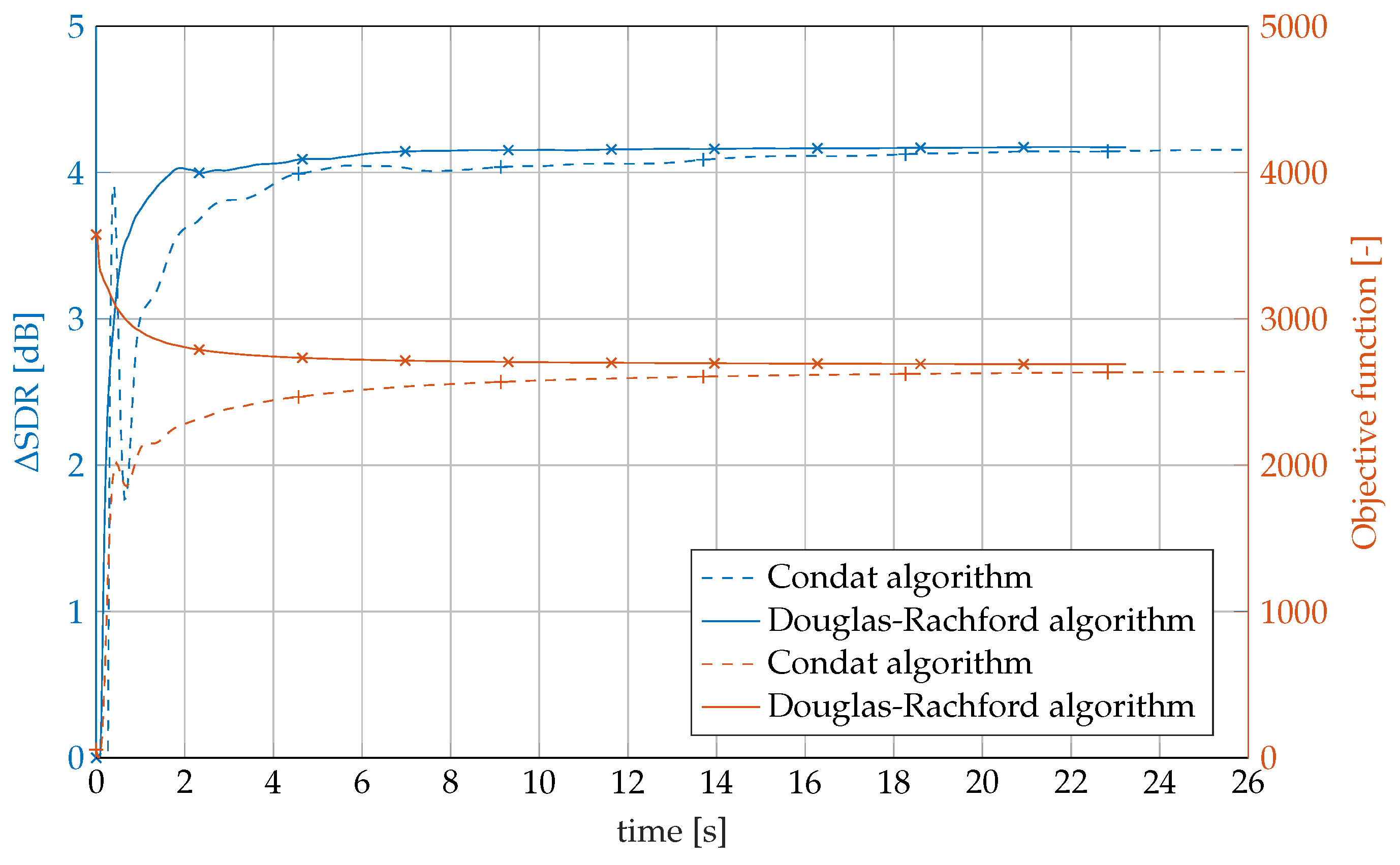
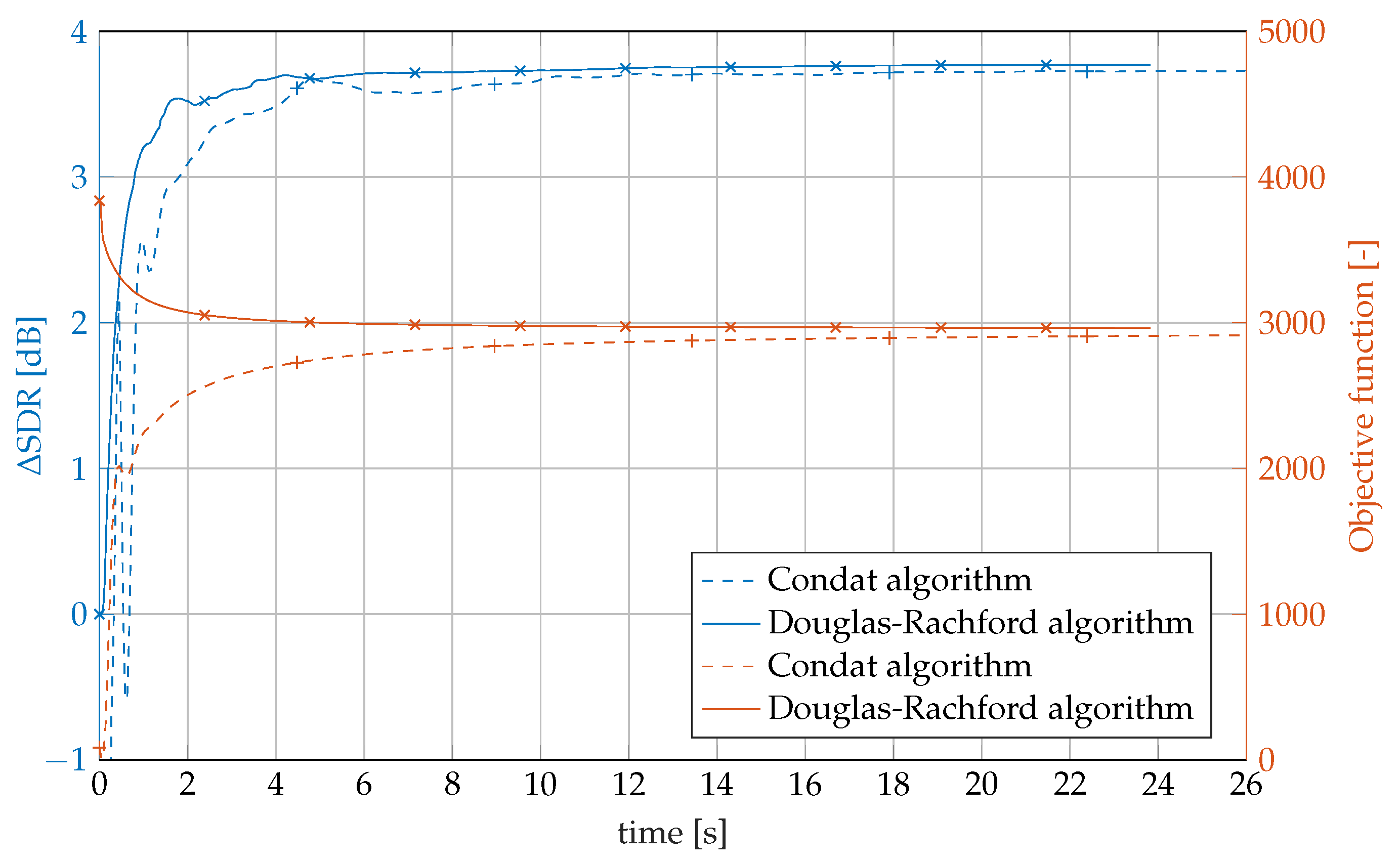
4.6. Comparison of the Algorithms

If converged, both presented algorithms produce the same solution when the objective function is strictly convex ([56], Part B1). In our case, Equation (24) is not strictly convex due to the 1 -norm, and therefore we can hardly hope for the same minimizers output from CA and DR. The objective function, i.e., the 1 -norm of coefficients, should coincide, however.
Regarding the computational cost, the CA (see Algorithm 1) requires, per iteration:
  • Sparsifying step: one soft thresholding, which is performed elementwise, and thus it is O ( N ) , and one analysis G * , which is O ( N log N )
  • Reliable part: one synthesis G and one analysis G * , both O ( N log N )
  • Each of the clipped parts: one synthesis, O ( N log N ) , and one elementwise projection, O ( N ) .
We neglect simple addition of vectors and multiplication of a vector with a scalar, and it is assumed that, where applicable, parts of the formulas are precomputed. It is clear that the overall cost is dominated by the transforms, namely every iteration requires three applications of G and two of G * .
On the other hand, the DR (see Algorithm 2) requires:
  • Sparsifying step: one soft thresholding, which is O ( N )
  • Projection onto K: one synthesis G and one pseudoinverse G + , which is in the order of G * , i.e., O ( N log N ) in our particular setup; projection that is performed elementwise, O ( N ) .
Again, the overall cost is dominated by the transforms, but we can see that the DR is much less demanding per iteration. Notice that this does not automatically mean that it will converge more quickly. We provide an experiment on this issue later.
The CA is a primal–dual method ([1], Ch. 5) and needs more memory than the DR does since variables in the dual space have to be kept, compared to the DR. The ratio of the memory requirements of the two algorithms depends also on the redundancy of the transform G * , i.e., on the ratio M / N .
The practical advantage of the DR lies also in the fact that only one step size has to be hand-tuned instead of two in the CA.

4.7. Redundancy of the Real-Part Operator
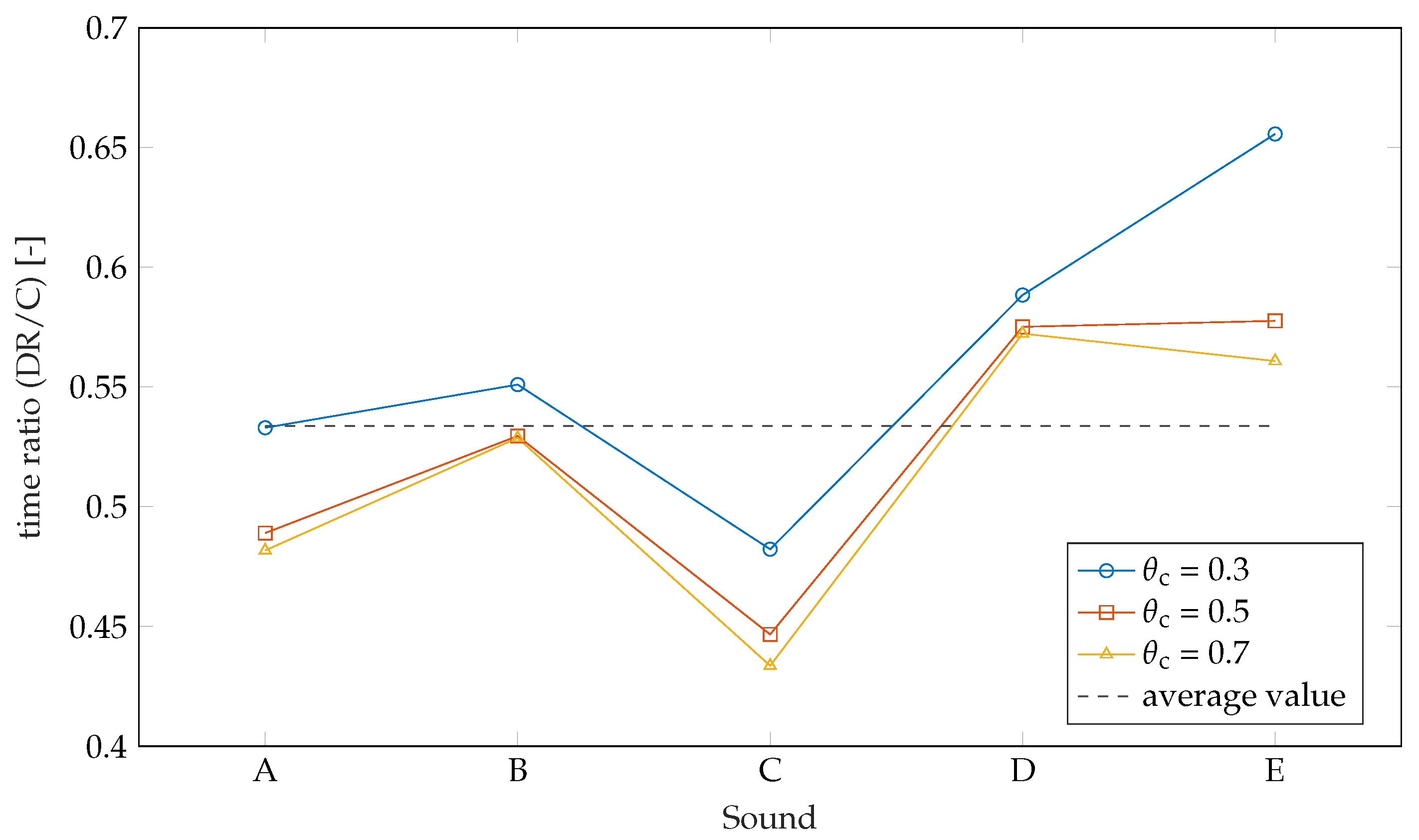
The operator ( · ) can be omitted in Equations (11) and (32) if its argument is real. As mentioned several times above, if the coefficient vector c ( K Q × × K Q ) ( C Q × × C Q ) , then the synthesis G c is real. It remains to check whether there exists an operation in any of the above algorithms that would make the coefficients fall out of this subspace: The soft thresholding is harmless in this regard. In the consolidated projection in Equation (31), G + = G * ( G G * ) 1 has the same complex-conjugate structure as G * since G G * is a real diagonal matrix, according to the assumption. In the projection in Equation (27) onto the reliable set, it is straightforward to see that, if the input coefficients belong to K Q × × K Q , then the same holds for the output, since ( M R G G * M R ) is a real diagonal matrix.

4.8. Results

For the following experiments, five audio excerpts sampled at 16 kHz with length of approximately 5 s were chosen. Because the goal of the experiments was the proof of concept demonstrating the convenience of the proposed projector in a practical example, rather than developing a novel method for audio declipping outperforming the current state of the art, these audio excerpts are fully sufficient for this purpose. Used signals differ in tonal content and sparsity with respect to the used time–frequency representation to cover a wide spectrum of audio signals; they consists of recordings of acoustic guitar, double bass, artificial signature tone, speech and string orchestra.
As a preprocessing step, the signals were peak-normalized and then artificially clipped to multiple thresholds θ c { 0 . 3 , 0 . 5 , 0 . 7 } . The clipping was considered to be symmetric, i.e., θ c = θ H = θ L .
Regarding the used transform, the common setting for audio declipping on 16 kHz sampled signals was adopted, i.e., the Gabor transform (STFT) with 1024-sample long Hann window (corresponding to 64 ms) and a 75% overlap. In all cases, the number of frequency channels was the same as the window length, i.e., Q = 1024 , except for the experiment shown in Figure 5, where the number of frequency channels was twice as many as the window length, specifically 2048 channels. In both settings, it holds that G G * = Id .
It has been noticed that the convergence performance of Algorithms 1 and 2 is influenced by the setting of parameters. These parameters were manually tuned such that both declipping algorithms performed well for all testing audio excerpts and all clipping thresholds. Specifically, the parameters of the CA were set to τ = 0 . 5 and σ = 0 . 666 and the DR parameter γ was set to 1.
The results were evaluated using Δ SDR , the signal-to-distortion ratio improvement, which is the difference between SDR of the restored signal and SDR of the clipped signal. Formally,
Δ SDR = SDR ( y , y ^ ) SDR ( y , y c ) ,
where y denotes the original (undistorted, ground-truth) signal, y ^ represents the restored signal and y c represents the clipped signal, while the SDR is the standard ratio computed as
SDR ( u , v ) = 10 log 10 u 2 2 u v 2 2 [ dB ] .
Figure 2 and Figure 3 are designed to demonstrate how the Condat algorithm and the Douglas–Rachford algorithm act over time, therefore the development of the Δ SDR and the objective function ( 1 -norm of the coefficients c ) for both algorithms are presented in these figures. Whereas Figure 2 displays only data obtained from reconstructing the “acoustic guitar” excerpt clipped at the level of 0.3, Figure 3 uses the average of all five audio signals and three tested clipping thresholds. It can be concluded from the figures that the objective function somewhat correlates with the Δ SDR curve and both cases show that both algorithms converge to the solution with the same final objective function value, but the DR algorithm converges more quickly, i.e., the curves level up more quickly, reaching slightly higher Δ SDR value. This is caused most likely by the projection step, where, in the CA, there are three individual projections (onto R, H and L) combined in a sum, thus it is not as accurate as in the DR case, where the projection step in Equation (31) is exploited.
The horizontal axis was converted to time in seconds in the figures, but they also offer an overview of the number of iterations, since the iterations of CA and DR do not consume the same amount of time. For this reason, apart from the Δ SDR and objective function graphs, the (+ and ×) markers emphasizing every 100th iteration are also displayed in the plots. Note that, although both algorithms ran for exactly 1000 iterations, since the time axis is limited to 26 s, only 570 iterations of the Condat algorithm are shown in Figure 2, and 581 iterations in Figure 3.
The average computational times for all sound excerpts and all computed clipping thresholds with a fixed number of 1000 iterations were 44.73 s for the CA and 23.82 s for the DR.
More detailed time comparison of both algorithms can be seen in Figure 4 and Figure 5 where the time ratio (time of DR divided by the time of CA) is plotted for every sound excerpt and clipping threshold θ c combination. Here, both algorithms ran until the objective function differed by 0.1% from the state of full convergence, the assessment of which was determined to be reached after exactly 3000 iterations. With the average value of the plotted time ratios being ca. 0.53, it is possible to claim that the DR algorithm is about twice as fast as the CA.
Figure 5 presents the same time ratios as Figure 4 with only one difference—the number of frequency channels of the Gabor transform is set to 2048 instead of 1024. The average value of the time ratio is now around 0.42. It can be assumed that, the more DGT coefficients we work with (longer windows, bigger overlaps or more frequency channels), the more significant time difference between the two algorithms there would be.
The algorithms were implemented and tested in MATLAB R2017a using the LTFAT toolbox [51,57] and, supporting the idea of reproducible research, the codes are available at http://www.utko.feec.vutbr.cz/~rajmic/software/project_accel_declip.zip in supplementary. All experiments ran on a PC with Intel i7-3770 3.4 GHz, 24 GB RAM and OS Windows 10 Pro (version 1809).

4.9. Other Applications

The new lemma is useful in situations where a problem to be solved requires projecting onto the box-type feasible set Γ as defined in Equation (), under the condition that L : C N C M with M N and L L * is a diagonal operator. Such a setup corresponds to the “painless” operator L as the operator that is used to synthesize the signal from its coefficients.
As the natural extension of the audio declipping problem, the image desaturation (i.e., recovering images that have been “clipped” to the maximum value due to a low dynamical range of a digital system) can benefit from the lemma as well. In a similar fashion, our projection can be used to keep the processed signal (or image) in a prescribed dynamic range, as present in the example in [11]. Dequantization is another example: each quantized signal sample has its origin in one of the non-overlapping intervals and our lemma is suitable to find signal coefficients that are consistent with the quantized observation [58]. As the last example, we name the signal inpainting problem, where a portion of samples is completely missing, while the others are considered reliable [35,50,59]. In this problem, nothing is directly known about the missing samples, thus the set Γ is defined such that the lower and upper bounds are set to minus and plus infinity, respectively; with this definition, projection lemma can be used here as well.

5. Conclusions

A new projector onto a box-shaped convex set in the transformed domain is presented in this article. The projector forms a generalization of previous results and its use was demonstrated on a simple audio signal declipping task.

Supplementary Materials

The following are available online at https://www.mdpi.com/2075-1680/8/3/105/s1.

Author Contributions

Conceptualization and methodology, P.R.; formal analysis, V.V. and O.M.; software, experiments, and visualization of results, P.Z.; and draft preparation, review and editing, P.R., V.V., P.Z. and O.M.

Funding

The work was supported by the joint project of the FWF and the Czech Science Foundation (GAČR): numbers I 3067-N30 and 17-33798L, respectively. Research described in this paper was financed by the National Sustainability Program under grant LO1401. Infrastructure of the SIX Center was used.

Acknowledgments

The authors thank Petr Sysel, Nicki Holighaus and Zdeněk Průša for discussing parts of the draft.

Conflicts of Interest

The authors declare no conflict of interest. The funders had no role in the design of the study; in the collection, analyses, or interpretation of data; in the writing of the manuscript, or in the decision to publish the results.

Abbreviations

The following abbreviations are used in this manuscript:
CACondat Algorithm
DCTDiscrete Cosine Transform
DFTDiscrete Fourier Transform
DGTDiscrete Gabor Transform
DRDouglas–Rachford (algorithm)
FBB-PDForward–Backward-Based Primal–Dual (algorithm)
FFTFast Fourier Transform
MDCTModified Discrete Cosine Transform
PAProximal Algorithm
SDRSignal-to-Distortion Ratio
STFTShort-Time Fourier Transform

References

  1. Boyd, S.P.; Vandenberghe, L. Convex Optimization; Cambridge University Press: Cambridge, UK, 2004. [Google Scholar]
  2. Combettes, P.; Pesquet, J. Proximal splitting methods in signal processing. In Fixed-Point Algorithms for Inverse Problems in Science and Engineering; Springer: New York, NY, USA, 2011; pp. 185–212. [Google Scholar]
  3. Bauschke, H.H.; Combettes, P.L. Convex Analysis and Monotone Operator Theory in Hilbert Spaces, 2nd ed.; Springer: Cham, Switzerland, 2011. [Google Scholar]
  4. Bayram, I. On the convergence of the iterative shrinkage/thresholding algorithm with a weakly convex penalty. IEEE Trans. Signal Process. 2016, 64, 1597–1608. [Google Scholar] [CrossRef]
  5. Chambolle, A.; Pock, T. A first-order primal-dual algorithm for convex problems with applications to imaging. J. Math. Imaging Vis. 2011, 40, 120–145. [Google Scholar] [CrossRef]
  6. Komodakis, N.; Pesquet, J. Playing with duality: An overview of recent primal-dual approaches for solving large-scale optimization problems. IEEE Signal Process. Mag. 2015, 32, 31–54. [Google Scholar] [CrossRef]
  7. Condat, L. A primal-dual splitting method for convex optimization involving Lipschitzian, proximable and linear composite terms. J. Optim. Theory Appl. 2013, 158, 460–479. [Google Scholar] [CrossRef]
  8. Selesnick, I.W.; Parekh, A.; Bayram, I. Convex 1-D total variation denoising with non-convex regularization. IEEE Signal Process. Lett. 2015, 22, 141–144. [Google Scholar] [CrossRef]
  9. Boyd, S.P.; Parikh, N.; Chu, E.; Peleato, B.; Eckstein, J. Distributed optimization and statistical learning via the alternating direction method of multipliers. Found. Trends Mach. Learn. 2011, 3, 1–122. [Google Scholar] [CrossRef]
  10. Daňková, M.; Rajmic, P.; Jiřík, R. Acceleration of perfusion MRI using locally low-rank plus sparse model. In Latent Variable Analysis and Signal Separation; Springer: Liberec, Czech Republic, 2015; pp. 514–521. [Google Scholar]
  11. Condat, L. A generic proximal algorithm for convex optimization—Application to total variation minimization. Signal Process. Lett. IEEE 2014, 21, 985–989. [Google Scholar] [CrossRef]
  12. Fadili, M.; Starck, J.L. Monotone operator splitting for optimization problems in sparse recovery. In Proceedings of the 2009 16th IEEE International Conference on Image Processing, Piscataway, NJ, USA, 7–10 November 2009; pp. 1461–1464. [Google Scholar]
  13. Combettes, P.; Pesquet, J. A Douglas–Rachford splitting approach to nonsmooth convex variational signal recovery. IEEE J. Sel. Top. Signal Process. 2007, 1, 564–574. [Google Scholar] [CrossRef]
  14. Šorel, M.; Bartoš, M. Efficient JPEG decompression by the alternating direction method of multipliers. In Proceedings of the 2016 23rd International Conference on Pattern Recognition (ICPR), Cancun, Mexico, 4–8 December 2016; pp. 271–276. [Google Scholar] [CrossRef]
  15. Combettes, P.; Wajs, V. Signal recovery by proximal forward-backward splitting. Multiscale Model. Simul. 2005, 4, 1168–1200. [Google Scholar] [CrossRef]
  16. Moreau, J.J. Proximité et dualité dans un espace hilbertien. Bull. Soc. Math. Fr. 1965, 93, 273–299. [Google Scholar] [CrossRef]
  17. Christensen, O. Frames and Bases, an Introductory Course; Birkhäuser: Boston, MA, USA, 2008. [Google Scholar]
  18. Christensen, O. An Introduction to Frames and Riesz Bases; Birkhäuser: Boston, MA, USA; Basel, Switzerland; Berlin, Germany, 2003. [Google Scholar]
  19. Gröchenig, K. Foundations of Time-Frequency Analysis; Birkhäuser: Basel, Switzerland, 2001. [Google Scholar]
  20. Balazs, P.; Dörfler, M.; Jaillet, F.; Holighaus, N.; Velasco, G. Theory, implementation and applications of nonstationary Gabor frames. J. Comput. Appl. Math. 2011, 236, 1481–1496. [Google Scholar] [CrossRef] [PubMed] [Green Version]
  21. Necciari, T.; Balazs, P.; Holighaus, N.; Søndergaard, P.L. The ERBlet transform: An auditory-based time-frequency representation with perfect reconstruction. In Proceedings of the 2013 IEEE International Conference on Acoustics, Speech and Signal Processing (ICASSP), Vancouver, BC, Canada, 26–30 May 2013; pp. 498–502. [Google Scholar] [CrossRef]
  22. Meyer, C.D. Matrix Analysis and Aplied Linear Algebra; SIAM: Philadelphia, PA, USA, 2000. [Google Scholar]
  23. Gröchenig, K. Non-uniform sampling in higher dimensions: From trigonometric polynomials to bandlimited functions. In Modern Sampling Theory: Mathematics and Applications; Benedetto, J.J., Ferreira, P.J.S.G., Eds.; Birkhäuser Boston: Boston, MA, USA, 2001; pp. 155–171. [Google Scholar] [CrossRef]
  24. Bogdanova, I.; Vandergheynst, P.; Antoine, J.P.; Jacques, L.; Morvidone, M. Stereographic wavelet frames on the sphere. Appl. Comput. Harmon. Anal. 2005, 19, 223–252. [Google Scholar] [CrossRef] [Green Version]
  25. Adcock, B.; Gataric, M.; Hansen, A.C. Weighted frames of exponentials and stable recovery of multidimensional functions from nonuniform Fourier samples. Appl. Comput. Harmon. Anal. 2017, 42, 508–535. [Google Scholar] [CrossRef] [Green Version]
  26. Daubechies, I.; Grossmann, A.; Meyer, Y. Painless nonorthogonal expansions. J. Math. Phys. 1986, 27, 1271–1283. [Google Scholar] [CrossRef]
  27. Wickerhauser, M.V. Mathematics for Multimedia; Birkhäuser: Boston, MA, USA, 2009. [Google Scholar]
  28. Vetterli, M.; Kovačević, J.; Goyal, V. Foundations of Signal Processing; Cambridge University Press: Cambridge, UK, 2014. [Google Scholar]
  29. Zölzer, U. DAFX: Digital Audio Effects, 2nd ed.; Wiley: New York, NY, USA, 2011. [Google Scholar]
  30. Etter, W. Restoration of a discrete-time signal segment by interpolation based on the left-sided and right-sided autoregressive parameters. IEEE Trans. Signal Process. 1996, 44, 1124–1135. [Google Scholar] [CrossRef]
  31. Abel, J.; Smith, J. Restoring a clipped signal. In Proceedings of the 1991 ICASSP-91 International Conference on Acoustics, Speech, and Signal Processing, Toronto, ON, Canada, 14–17 May 1991; Volume 3, pp. 1745–1748. [Google Scholar] [CrossRef]
  32. Dahimene, A.; Noureddine, M.; Azrar, A. A simple algorithm for the restoration of clipped speech signal. Informatica 2008, 32, 183–188. [Google Scholar]
  33. Selesnick, I. Least squares with examples in signal processing. OpenStax CNX. 2013. Available online: https://cnx.org/contents/XRPKcVgh@1/Least-Squares-with-Examples-in-Signal-Processing (accessed on 14 September 2019).
  34. Bilen, Ç.; Ozerov, A.; Pérez, P. Audio declipping via nonnegative matrix factorization. In Proceedings of the 2015 IEEE Workshop on Applications of Signal Processing to Audio and Acoustics (WASPAA), New Paltz, NY, USA, 18–21 October 2015; pp. 1–5. [Google Scholar] [CrossRef]
  35. Adler, A.; Emiya, V.; Jafari, M.; Elad, M.; Gribonval, R.; Plumbley, M. Audio Inpainting. IEEE Trans. Audio Speech Lang. Process. 2012, 20, 922–932. [Google Scholar] [CrossRef]
  36. Adler, A.; Emiya, V.; Jafari, M.; Elad, M.; Gribonval, R.; Plumbley, M. A constrained matching pursuit approach to audio declipping. In Proceedings of the 2011 IEEE International Conference on Acoustics, Speech and Signal Processing (ICASSP), Prague, Czech Republic, 22–27 May 2011; pp. 329–332. [Google Scholar] [CrossRef]
  37. Defraene, B.; Mansour, N.; Hertogh, S.D.; van Waterschoot, T.; Diehl, M.; Moonen, M. Declipping of audio signals using perceptual compressed sensing. IEEE Trans. Audio Speech Lang. Process. 2013, 21, 2627–2637. [Google Scholar] [CrossRef]
  38. Siedenburg, K.; Kowalski, M.; Dorfler, M. Audio declipping with social sparsity. In Proceedings of the 2014 IEEE International Conference on IEEE Acoustics, Speech and Signal Processing (ICASSP), Florence, Italy, 4–9 May 2014; pp. 1577–1581. [Google Scholar]
  39. Kitić, S.; Jacques, L.; Madhu, N.; Hopwood, M.; Spriet, A.; De Vleeschouwer, C. Consistent iterative hard thresholding for signal declipping. In Proceedings of the 2013 IEEE International Conference on Acoustics, Speech and Signal Processing (ICASSP), Vancouver, BC, Canada, 26–30 May 2013; pp. 5939–5943. [Google Scholar] [CrossRef]
  40. Kitić, S.; Bertin, N.; Gribonval, R. Audio declipping by cosparse hard thresholding. In Proceedings of the 2nd Traveling Workshop on Interactions between Sparse models and Technology, Namur, Belgium, 27–29 August 2014. [Google Scholar]
  41. Kitić, S.; Bertin, N.; Gribonval, R. Sparsity and cosparsity for audio declipping: A flexible non-convex approach. In LVA/ICA 2015—The 12th International Conference on Latent Variable Analysis and Signal Separation; Springer: Liberec, Czech Republic, 2015. [Google Scholar]
  42. Záviška, P.; Rajmic, P.; Průša, Z.; Veselý, V. Revisiting synthesis model in sparse audio declipper. In LVA/ICA 2018—The 14th International Conference on Latent Variable Analysis and Signal Separation; Springer: Guildford, UK, 2018; pp. 429–445. [Google Scholar] [CrossRef]
  43. Záviška, P.; Rajmic, P.; Mokrý, O.; Průša, Z. A proper version of synthesis-based sparse audio declipper. In Proceedings of the 2019 IEEE International Conference on Acoustics, Speech and Signal Processing (ICASSP), Brighton, UK, 12–17 May 2019; pp. 591–595. [Google Scholar] [CrossRef]
  44. Weinstein, A.J.; Wakin, M.B. Recovering a clipped signal in sparseland. Sampl. Theory Signal Image Process. 2013, 12, 55–69. [Google Scholar]
  45. Siedenburg, K.; Dörfler, M. Structured sparsity for audio signals. In Proceedings of the 14th International Conference on Digital Audio Effects (DAFx-11), Paris, France, 19–23 September 2011; pp. 23–26. [Google Scholar]
  46. Kowalski, M.; Siedenburg, K.; Dörfler, M. Social sparsity! Neighborhood systems enrich structured shrinkage operators. IEEE Trans. Signal Process. 2013, 61, 2498–2511. [Google Scholar] [CrossRef]
  47. Donoho, D.L.; Elad, M. Optimally sparse representation in general (nonorthogonal) dictionaries via 1 minimization. Proc. Natl. Acad. Sci. USA 2003, 100, 2197–2202. [Google Scholar] [CrossRef] [PubMed]
  48. Bayram, I.; Kamasak, M. A simple prior for audio signals. IEEE Trans. Acoust. Speech Signal Process. 2013, 21, 1190–1200. [Google Scholar] [CrossRef]
  49. Bayram, I.; Akykıldız, D. Primal-dual algorithms for audio decomposition using mixed norms. Signal Image Video Process. 2014, 8, 95–110. [Google Scholar] [CrossRef]
  50. Rajmic, P.; Bartlová, H.; Průša, Z.; Holighaus, N. Acceleration of audio inpainting by support restriction. In Proceedings of the 7th International Congress on Ultra Modern Telecommunications and Control Systems, Brno, Czech Republic, 6–8 October 2015. [Google Scholar]
  51. Søndergaard, P.L.; Torrésani, B.; Balazs, P. The linear time frequency analysis toolbox. Int. J. Wavelets Multiresolution Anal. Inf. Process. 2012, 10. [Google Scholar] [CrossRef]
  52. Holighaus, N.; Wiesmeyr, C. A class of warped filter bank frames tailored to non-linear frequency scales. arXiv 2016, arXiv:1409.7203. [Google Scholar]
  53. Donoho, D. De-noising by soft-thresholding. IEEE Trans. Inf. Theory 1995, 41, 613–627. [Google Scholar] [CrossRef]
  54. Bruckstein, A.M.; Donoho, D.L.; Elad, M. From sparse solutions of systems of equations to sparse modeling of signals and images. SIAM Rev. 2009, 51, 34–81. [Google Scholar] [CrossRef]
  55. Rajmic, P. Exact risk analysis of wavelet spectrum thresholding rules. In Proceedings of the 2003 10th IEEE International Conference on Electronics, Circuits and Systems, Sharjah, United Arab Emirates, 14–17 December 2003; Volume 2, pp. 455–458. [Google Scholar] [CrossRef]
  56. Hiriart-Urruty, J.B.; Lemaréchal, C. Fundamentals of Convex Analysis; Springer: New York, NY, USA, 2001. [Google Scholar]
  57. Průša, Z.; Søndergaard, P.L.; Holighaus, N.; Wiesmeyr, C.; Balazs, P. The large time-frequency analysis toolbox 2.0. In Sound, Music, and Motion; Aramaki, M., Derrien, O., Kronland-Martinet, R., Ystad, S., Eds.; Lecture Notes in Computer Science; Springer International Publishing: Cham, Switzerland, 2014; pp. 419–442. [Google Scholar]
  58. Rencker, L.; Bach, F.; Wang, W.; Plumbley, M.D. Fast iterative shrinkage for signal declipping and dequantization. In Proceedings of the iTWIST’18—International Traveling Workshop on Interactions between Low-Complexity Data Models and Sensing Techniques, Marseille, France, 21–23 November 2018. [Google Scholar]
  59. Mokrý, O.; Záviška, P.; Rajmic, P.; Veselý, V. Introducing SPAIN (SParse Audio INpainter). In Proceedings of the 27th European Signal Processing Conference (EUSIPCO), A Coruña, Spain, 2–6 September 2019. [Google Scholar]
Figure 1. Illustration of the inequality in Equation (18) for different cases of the relative position of L z and the interval [ b 1 , b 2 ] . Only a single entry is depicted for each vector, i.e., the meaning of L z in the plot is ( L z ) m and similarly for the other vectors. The point L ( z v ) represents an arbitrary point in the interval [ b 1 , b 2 ] , as assumed.
Axioms 08 00105 g001
Figure 2. Development of the Δ SDR (blue) and objective function (orange) through iterations for the particular “acoustic guitar” excerpt and the clipping threshold θ c = 0 . 3 . Both algorithms ran for a fixed number of 1000 iterations here. To demonstrate the time differences between the algorithms, every 100th iteration is emphasized with a marker (+ for Condat and × for Douglas–Rachford).
Axioms 08 00105 g002
Figure 3. Analog to Figure 2, development of the Δ SDR (blue) and objective function (orange) through iterations is shown, but now averaged over the testing sounds and the clipping thresholds. The number of iterations was 1000.
Axioms 08 00105 g003
Figure 4. Relative elapsed time, Douglas–Rachford versus Condat algorithm, for all testing sounds and clipping thresholds. Both algorithms were first let to fully converge, which was in practice observed after 3000 iterations. Then, both algorithms ran again until the objective function differed by 0.1% from the respective solutions. The Gabor transform with 1024-sample long Hann window and 1024 frequency channels with 75% overlap was used.
Axioms 08 00105 g004
Figure 5. Analog to Figure 4, this picture presents relative running times of the Douglas–Rachford versus Condat algorithm. The only difference is that the Gabor transform now uses 2048 frequency channels.
Axioms 08 00105 g005

