

Dynamic Simulation of Cracked Spiral Bevel Gear Pair Considering Assembly Errors


1
School of Mechanical Engineering and Automation, Northeastern University, Shenyang 110819, China
2
Key Laboratory of Vibration and Control of Aero-Propulsion Systems Ministry of Education of China, Northeastern University, Shenyang 110819, China
3
AVIC Shenyang Engine Design Institute, Shenyang 110066, China
4
AECC Sichuan Gas Turbine Establishment, Chengdu 610500, China
5
National Key Laboratory of Science and Technology on Helicopter Transmission, Nanjing University of Aeronautics and Astronautics, Nanjing 210016, China
*
Author to whom correspondence should be addressed.
Machines 2022, 10(10), 929; https://doi.org/10.3390/machines10100929
Submission received: 29 August 2022
/
Revised: 8 October 2022
/
Accepted: 11 October 2022
/
Published: 13 October 2022
(This article belongs to the Special Issue Dynamics Control and Vibration Monitoring in Industrial Machines)
Abstract
:The tooth root crack fault is a common fault type of the spiral bevel gear pair (SBGP). Affected by the strong bearing capacity, the early crack fault of the SBGP cannot be found in time. In this study, a finite element (FE) model of the SBGP is established and assembled through the tooth contact analysis. The maximum tooth root stress is analyzed considering the variation of assembly errors. Meanwhile, this study simulates the tooth root crack fault of the bevel pinion with different crack degrees. The initial position of the crack is located where the maximum tooth root stress appears. The time-varying mesh stiffness (TVMS) of the SBGP considering different degrees of the pinion tooth root crack fault is obtained. The TVMS and the non-load transmission error are brought into a hybrid FE dynamic model, and steady responses are solved. Based on this, the sensitivities of various statistical indicators for identifying the tooth root crack fault of SBGP under the influence of assembly errors are verified. This paper can provide the necessary theoretical basis for the analysis and diagnosis of tooth root crack faults in the SBGP transmission system.
1. Introduction
The transmission system of the SBGP has a strong load-bearing capacity, and minor cracks are not easy to be found in time, resulting in broken teeth after the cracks expand to the strength limit. From the example of the broken tooth fault shown in Figure 1, at the tooth root of the active flank, the crack is initiated in the middle position along the tooth width. The propagation path of the crack has different characteristics in different directions. Kim et al. [1] and Park [2] pointed out that in the tooth thickness direction, the crack propagates toward the gear foundation first, and when the crack propagates beyond the tooth centerline, the propagation direction turns to the root of the opposite flank. In the tooth width direction, the crack propagations towards the heel and toe directions have different performance characteristics. For the toe side, the propagation direction of the crack almost does not change along the propagation direction of the early crack. For the heel direction, the propagation direction keeps unchanged at first, then after a certain degree, the crack propagation direction turns towards the top of the tooth. Spievak et al. [3] proved this phenomenon by the principle of fracture mechanics. Based on this, Levicki et al. [4] studied the effect of moving the tooth load on the crack propagation path of bevel gears. Vukelic et al. [5] studied the fractured SBGP of a shipyard crane. They pointed out that gear crack failure may be caused by misalignments. Ural et al. [6] used the fracture mechanics method to accurately simulate the crack propagation direction of the SBGP compared with the actual broken tooth morphology of the OH-58 Kiowa Helicopter. In this paper, the FE method of the SBGP is established, and the influences of the assembly errors on the tooth root stress of the SBGP are analyzed. Meanwhile, based on the crack propagation law proposed by the previous literature, the crack fault at the tooth root of the pinion is simulated and the TVMS curves of the SBGP under different crack degrees considering the assembly errors are calculated.
The complex space surface structure of the SBGP makes it different from the spur gear pair or the helical gear pair, which can obtain the TVMS by the energy method [8,9]. The general research on the TVMS of the SBGP are mainly divided into the loaded tooth contact analysis method [10,11,12,13] and the FE method. The loaded tooth contact analysis method simplifies the gear local contact relationship and is obtained by the linear programming method [14]. The efficiency of this method is much higher than that of the FE method. Through this method, scholars have carried out research on gear pair machining parameter optimization [15,16,17], machining error influence analysis [18], assembly error influence analysis [19], system-level modelling [20] and so on. However, there were few studies about gear tooth fault simulation and tooth bending stress analysis by using this method. Due to the robustness of the contact analysis of the FE method, scholars have conducted many studies on the static and dynamic characteristics of the SBGP based on it. Bibel et al. [21] analyzed the tooth surface contact stress of SBGP by the FE method. Argyris et al. [22] analyzed the contact stress and bending stress of the SBGP by the FE method. Gonzalez-Perez et al. [23] established a FE model of the SBGP by reverse engineering, which well restored the designer’s intention. They simulated the tooth surface contact pattern and contact stress accurately through the FE model. Hou et al. [24] proposed the vector form intrinsic FE method, and based on this method, the static contact stress and bending stress of the SBGP were analyzed. They pointed out that when dealing with dynamic problems and strong nonlinear problems, the efficiency of the proposed model will be greatly improved. Gan et al. [25] studied the temperature distribution of the SBGP under the mixed electrohydrodynamic lubrication state based on the FE method. Fu et al. [26] established a FE model of the SBGP and analyzed the influence of input torque on the tooth bending stress, tooth surface contact stress and transmission error. Hou et al. [27] analyzed the contact stress and tooth bending stress changes of the SBGP considering different torques and different modulus by the FE method. They pointed out that under the influence of edge contact, the contact stress of the tooth surface will surge at the edge. Wang et al. [28] simulated the dynamic contact and impact phenomena of an SBGP based on an FE model. The maximum resonance frequency of the system was analyzed. Guo et al. [29] analyzed the tooth surface contact stress distribution before and after tool optimization by the FE method. This method can be used to eliminate edge contact and reduce the maximum contact stress under heavy load conditions. Wang et al. [30] established a coupled thermo-elastic 3D FE model to improve the thermal behavior of SBGP by adjusting the machine setting parameters. Yang et al. [31] considered the broken tooth fault of the SBGP, the TVMS was calculated by the FE method, and the dynamic response of the system is obtained by bringing it into the pure torsional dynamic model.
Through the above survey, it is found that the FE method is a common method used to analyze the bending stress and the contact stress of the SBGP. Hence, this paper analyzes the tooth root stress considering the variation of assembly errors to locate the initial crack position. Meanwhile, the TVMS curve of the SBGP under the pinion tooth crack fault condition is obtained by introducing a simple space crack into the FE model. Through the dynamic analysis, the system responses under different crack degrees are obtained. Based on this, the sensitivity of some statistical indicators for monitoring the crack fault of SBGP under the influence of assembly errors is verified.
2. FE Model Description
2.1. Tooth Contact Analysis Considering the Assembly Error
In this section, the teeth surfaces of the bevel pinion and the bevel gear are derived by the generation method and the tile method, respectively. The blank parameters can be seen in Table 1 and the machine tooth setting parameters of the bevel pinion and the bevel gear can be seen in Table 2 and Table 3, respectively.
Through the local synthesis method [32,33], the tooth surface points r1 and r2, and the tooth surface normal directions n1 and n2 of the pinion and the gear are obtained, respectively. The detail of the tooth surface derivation can refer to Appendix A. The following coordinate transformations are used to assemble the two gears into the same mounting coordinate system:
where i = 1, 2 represent the pinion and the gear, respectively; Mhi is the transformation matrix from the cutter head coordinate system to the blank coordinate system; Lhi is the first three-order sub-matrix of Mhi; ψci, si and θi are the rotation angle of the cradle, the distance from the point on the theoretical tool tip to the tool profile, and the rotation angle of the cutter head, respectively. Mhi can be expressed as:
where ΔE is the offset error; ΔΣ is the shaft angle error; ΔAp is the pinion axial error; ΔAg is the gear axial error. The assembly errors are expressed in Figure 2. φ1 and φ2 are the initial installation angles of the pinion and the gear, respectively; Σ is the shaft angle.
In the assembly coordinate system O-xh-yh-zh, the two meshing gear teeth should have collinear normal vectors and the same coordinate values at the contact point:
There are seven independent equations in the above equation system, including eight unknown parameters. Given the rotation angle of the pinion ψ1, other variables can be determined. Then, the contact trajectory and the non-load transmission error (NLTE) of the SBGP in the rotation range of ψ1 = (−π/z1, π/z1) are obtained. The transmission error between the two gears can be expressed as:
where ϕ10 and ϕ20 are the initial rotation angles of the pinion and the gear, respectively; ϕ1 and ϕ2 are the real-time rotation angles of the pinion and the gear, respectively; z1 and z2 are the numbers of teeth of the pinion and the gear, respectively.
It is known that for the SBGP, the NLTE is one of the main sources of vibration and noise. The smaller the NLTE is, the smoother the gear system operates. Based on the parameters of the SBGP listed in Ref. [34], the NLTEs and contact trajectories of the SBGP under different assembly error states are illustrated in Figure 3. Influenced by assembly errors, both the NLTE values and the contact trajectories of the SBGP have changed. For the parameters of the SBGP in this study, the larger the value of ΔE, ΔΣ and ΔAg become, the larger the value of NLTE becomes, and the smaller the value of ΔAp becomes, the larger the value of NLTE becomes. Therefore, in the process of assembling the SBGP, it is necessary to control these errors to obtain a smaller value of ΔE, ΔΣ and ΔAg, and a larger value of ΔAp to ensure that the NLTE values are as small as possible.
2.2. FE Modelling of the SBGP
The FE model of the SBGP is illustrated in Figure 4.
Since the FE model established in this paper is a five-tooth model and the actual gears foundation structures are not fully established (see Figure 4), a master node is used to constrain the nodes on the inner hub and the rigid surfaces of both sides of the pinion. The nodes on the bottom surface and the rigid surfaces of the gear are fully constrained. Five contact pairs are established among the mating tooth surfaces by the Conta 174 and Target 170 element pairs. A mesh cycle is divided into 20 positions. At each position, the rotation of the SBGP must meet the requirement of the transmission ratio; meanwhile, the pinion must rotate with an angle to close the NLTE. The nonlinear contact iteration is performed to complete the static analysis of the gear pair. After that, the equivalent static rotation angle θp1 of the master node along the rotation direction is obtained. The mesh stiffness value of the SBGP can be obtained by the following equation:
where T is the driving torque applied on the pinion; rp is the pitch circle radius of the SBGP. It is worth noting that the TVMS obtained in this paper is entirely caused by the contact deformation of the SBGP, so the changing of NLTE should be considered additionally in the subsequent dynamic analysis.
The TVMS of the SBGP in the healthy state can be seen in Figure 5.
2.3. Tooth Root Crack Fault Simulation
According to the results of Ref. [3], it can be seen that on the active tooth side, the crack originated at the midpoint along the tooth width of the tooth root. The crack propagation can be explained in two directions. In the tooth thickness direction, the crack expands to the foundation first, and after reaching the middle of the tooth, the expanding direction turns towards the root of the opposite flank. In the tooth width direction, the early cracks propagate parallel to the tooth width direction (see the shaded part in Figure 6). In this paper, the early tooth root crack fault of the pinion is simulated through the node replacement method (see Figure 7). Through the tooth root stress analysis, the position where the maximum tooth root stress of the pinion occurs is obtained. The crack initial position is usually happening where the maximum tooth root stress appears due to the lack of strength. The distance from the toe end to the crack initial position is set as λ. According to the simplified fault morphology, taking the initial position as the intermediate position, on the tooth root surface, the width of the crack along the tooth width direction is δ. The crack depth is specified as χ. The crack width gradually narrows with depth.
The flow chart of the FE modelling process is shown in Figure 8.
3. Results and Discussion
3.1. Influence of the Assembly Errors on the Tooth Root Stress Distribution
The direct cause of tooth root crack fault is that the root stress exceeds the material bearing limit. Therefore, the position where the crack initiates should be where the root stress is the largest. Affected by the assembly errors, the maximum tooth root stress value and its position are volatile. In order to explore the influences of assembly errors on the maximum root stress value and its position, the following research is carried out.
After the static analysis, the von Mises stress cloud contour of the pinion in the error-free condition is shown in Figure 9. Based on the mesh layer where the maximum von Mises stress of the tooth root is located (the red line in the figure), all nodes on the red line are extracted and the relative von Mises stress is obtained. After three meshing cycles (a single tooth goes through the entire cycle of meshing in and out), the contour plots of the stress variation of the selected nodes under different assembly error conditions are analyzed below.
3.1.1. Offset Error
As shown in Figure 10, with the increase in ΔE, the maximum von Mises stress of the tooth root of the pinion increases gradually. When ΔE raises in the positive direction, the maximum stress value increases faster, which indicates that to avoid the excessive maximum stress value of the tooth root of the pinion, it should avoid the too large positive value of ΔE. The position of the maximum root stress will gradually change towards toe with the increase in ΔE because the contact trajectory will gradually move towards toe with the increase in ΔE. In general, to reduce the maximum value of the root stress of the pinion, the variation of ΔE should not be too large.
3.1.2. Shaft Angle Error
The influence of ΔΣ on the maximum root stress value and its position is shown in Figure 11. It can be seen from the figure that with the gradually increase in ΔΣ, the maximum root stress shows a gradually increasing trend. However, in the range of ΔΣ varying from −0.1° to 0.1°, the position variation of the maximum root stress is not obvious, which indicates that the position of the maximum root stress is not sensitive to the changing of ΔΣ.
3.1.3. Pinion Axial Error
The influence of ΔAp on the maximum root stress value and its position is illustrated in Figure 12. It can be seen from the figure that the smaller the value of ΔAp, the greater the maximum root stress. However, no matter how much ΔAp changes, it does not affect the position where the maximum root stress occurs.
3.1.4. Gear Axial Error
Figure 13 illustrates the influence of ΔAg on the maximum root stress value of the pinion and its position along the tooth width. It can be seen from the figure that with the increase in ΔAg, the position of the maximum tooth root stress of the pinion moves towards the toe direction. However, within the range of ΔAg = −0.1 mm to 0.1 mm, the maximum tooth root stress value only increased by 6.5 MPa. This indicates that the maximum root stress of the pinion is insensitive to the change in ΔAg.
In general, among all the assembly errors, ΔE has the greatest influence on the position of the maximum root stress of the pinion, whereas ΔAg has the least. Within the scope of ensuring the reasonable root stress of the mating gear, the changes of ΔE, ΔΣ and ΔAp should be especially controlled. The smaller the value of ΔE and ΔΣ are, the better it is to obtain a small root stress value. The larger the value of ΔAp becomes, the better it is to obtain a small root stress value. No matter how the assembly error changes in this study, the maximum root stress always appears around the middle of the tooth width and deviates from the toe side. This shows that the root crack fault of the pinion is most likely to occur around this zone.
3.2. Crack Fault Analysis of the SBGP
3.2.1. TVMS Due to the Crack Fault
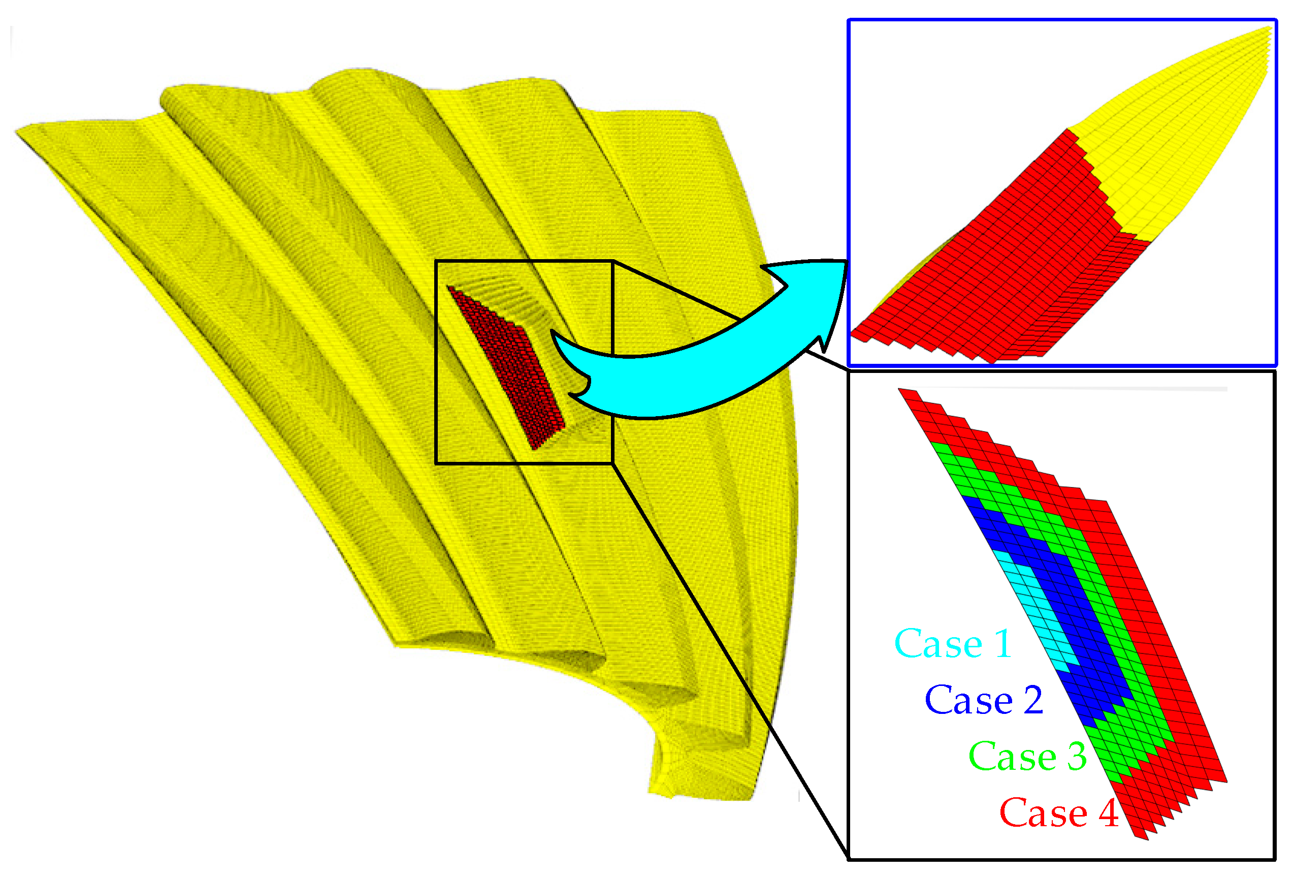
The early cracks propagated nearly parallel to the tooth width direction. In this study, the tooth root crack of the SBGP is divided into four working cases. The crack cross-section morphology is shown in Figure 14. Through the above results of the root stress distribution in the healthy state, it is assumed that the initial crack of the tooth root occurs at the position of the maximum stress (λ = 29.2 mm). Case 1 represents the initial crack. Case 2 and Case 3 represent the further aggravation of the crack fault, in which the crack morphology increases in both length δ and depth χ. Finally, Case 4 indicates that the crack has crossed the centerline of the tooth and has begun to turn its direction and propagate towards the root of the opposite side. The location and the morphology parameters of the four cases are listed in Table 4 and Figure 14.
Based on the method described in Section 2, Figure 15a shows the TVMS curves of the SBGP under different degrees of crack faults. It can be seen from the figure that when a tooth root crack fault occurs, two meshing cycles of the TVMS curves are affected. Figure 15b illustrates the initial gaps of all five tooth pairs over two meshing cycles. It is worth noting that the root crack fault is artificially implanted at the tooth root of the pinion of tooth pair 3. Here, the two meshing cycles are divided into three parts according to the change of the tooth pair with the smallest initial gap. The first part is when tooth pair 2 has the smallest absolute initial gap value. During this period, tooth pair 1 exits the meshing state, the absolute value of the initial gaps of tooth pair 3 decreases gradually, and the absolute value of the initial gaps of tooth pair 2 increases gradually. For tooth pair 3, the crack is not directly below the contact ellipse currently, so the TVMS is less affected by the crack fault. When the absolute value of the initial gaps of tooth pair 3 among all the tooth pairs is the smallest, tooth pair 2 gradually exits the meshing state, and tooth pair 4 gradually enters the meshing state. At this time, the contact force is mostly endured by tooth pair 3, and the contact ellipse is above the root crack. Therefore, the TVMS in this period is mostly affected by the crack fault. The stiffness value of Case 4 in this region can reach a maximum relative difference of 5.45% compared with the healthy condition. When the minimum initial gap exists on the tooth pair 4, the tooth pair 3 is about to leave or has already left the meshing state, and the tooth pair 5 is about to enter or has entered the meshing state. During this period, the contact force endured by tooth pair 3 decreases gradually, and the contact ellipse leaves the tooth surface above the crack gradually. Therefore, the TVMS values of crack fault condition in this region tend to the curves of the healthy state.
3.2.2. Dynamic Simulation
A schematic of the SBGP and shafts system is established (see Figure 16). In this system, the driving torque and the slave torque are applied on the drive node and the slave node, respectively. The dimensions of the input shaft and the intermediate shaft, the supporting stiffnesses and damping coefficients of the gear, the supporting bearings B1, B2, B3, and B4, and the mass of the gear are referenced in Ref. [34].
The undamped equations of motions of the SBGP are as follows:
where mbi, Ibix, Ibiy and Ibiz are the mass and moments of inertia of the gear i (i = 1,2 represents the bevel pinion and bevel gear, respectively). kbix, kbiy, kbiz, kbiθx, kbiθy and kbiθz are the supporting stiffness of gear i in six directions, respectively. kb1b2 is the TVMS of the SBGP and NLTE is the NLTE of the SBGP accordingly. Considering the NLTE in the system means that only when the dynamic projected displacement of the SBGP exceeds the value of NLTE, the contact of the SBGP can occur. The derivation of the projection displacement vector of the SBGP δb1b2 can be seen in Ref. [34]. The superscript k of δkb1b2 denotes the k-th element of vector δb1b2. qb1b2 is the displacement vector consisting of 12 degrees of freedom of the two gears. Due to the introduction of the shaft components, the driving torque Tb1 originally added to the rotation direction of the pinion is transferred to the drive node of the input shaft. At the same time, the slave torque Tb2 originally added in the rotation direction of the gear is transferred to the slave node of the intermediate shaft. The schematic of the grouping of the system stiffness matrix and the damping matrix is illustrated in Figure 17.
The damping matrices of the input shaft-bevel pinion structure (with footnote “1”) and the damping matrices of the intermediate shaft-bevel gear structure (with footnote “2”) are described as:
where αi and βi are the damping coefficients of the structure i; Mi and Ki are the mass matrix and stiffness matrix of the structure i, which are solved by the Timoshenko beam theory. The damping of the supporting bearings is considered as contact values. The mesh damping of the SBGP is described as:
where ξ denotes the damping ratio of the gear pair, mb1 and mb2 are the mass of the bevel pinion and the bevel gear, respectively.
The system level equation of motions can be constructed as the matrix form:
In the simulation process, being as the excitation source, kb1b2 and NLTE are interpolated according to the time series relationship to obtain the mesh stiffness and NLTE values under each Newmark integration step. After solving for a whole sampling time, the dynamic response of the system is obtained.
3.2.3. Response Analysis Due to the Crack Fault of the SBGP
Figure 18 and Figure 19 illustrate the time-domain waveforms and amplitude spectrums of the pinion in the healthy condition and cracked Case 4 condition, respectively. It can be seen from the figures that in the healthy state, the acceleration time-domain waveforms of all meshing cycles are identical, and the components in the amplitude spectrums are only the meshing frequency fm and its harmonics. Under the crack fault condition, every time the pinion revolts one period Tbp, the faulty tooth participates in meshing for two mesh periods. There are fluctuations at intervals of Tbp in the time-domain waveform of Case 4. The fault causes the mutation waveform of three meshing cycles. In the faulty amplitude spectrum, under the influence of the crack fault, sidebands with the rotation frequency of the pinion fbp as the interval appear on both sides of the meshing frequency and its harmonics.
3.2.4. Sensitivity Analysis of Statistical Indicators under Healthy Condition
Based on the acceleration signal of bearing B3 in the y-direction, the time-domain statistical indicators are validated for detecting the crack fault and its severity. The statistical indicators [35] can be seen in Table 5.
It can be seen from the variation trends of multiple time-domain statistical indicators (see Figure 20) that when a tooth crack fault occurs, the values of the indicators A, SMR, P, C, I and L have monotonic changing trends relative to the health condition. So, these indicators can be used to monitor the severity of crack degrees.
Figure 21 illustrates the change of the frequency-domain indicators for the acceleration signal of bearing B3 in the y-direction under different crack degrees. The name and the expression of each indicator in the frequency domain can be referred to in Table 6.
As can be seen from Figure 21, when there is a crack fault at the tooth root of the pinion, the values of the frequency-domain indicators F12, F14, F15, F17, F18, F19, F22 and F23 have monotonic changes compared with the healthy ones, which indicates that the above frequency-domain indicators can clearly distinguish the severity of the crack degrees in the SBGP system. Therefore, these frequency-domain indicators can be used to diagnose root crack faults in the SBGP system.
3.2.5. Crack Fault Detection under the Influence of the Offset Errors
Assembly errors are unavoidable during the SBGP operation. To explore the sensitivity of the upper-mentioned indicators in diagnosing the crack fault of the SBGP under the influence of assembly errors, the following analysis is performed.
Through the analysis of Section 3.1, it is known that the offset error affects the position of the maximum tooth root stress the most. Therefore, the following discussion deals with the effectiveness of the indicators for diagnosing the crack fault under the influence of the offset error. First, the crack severities are still classified as four cases. The crack sizes remain unchanged (i.e., δ and χ follow the values of Case 1–Case 4 in Table 4). Under the influence of the offset error, the maximum root stress position has changed, so the position parameter of the cracks λ has changed (see Table 7).
The TVMS curves are shown in Figure 22. First, it can be seen from the healthy condition diagram (see Figure 22a) that as ΔE changes from −0.1 mm to 0.1 mm, the TVMS curves of the SBGP show an overall upward trend. Compared with the condition of ΔE = −0.1 mm, the maximum stiffness value increased by 5.09% and the minimum stiffness value increased by 3.47% under the condition of ΔE = 0.1 mm.
The effect of crack degrees on TVMS is analyzed for different offset errors. For ΔE varies from −0.1 mm to 0.1 mm, compared to the health condition, the max/min relative differences under various crack degrees are listed in Table 8. It can be seen from the table that with the increase in ΔE, the max/min relative differences values show an overall upward trend as the crack severity increases, which indicates that a higher offset error value may aggravate the meshing state of the SBGP with crack fault.
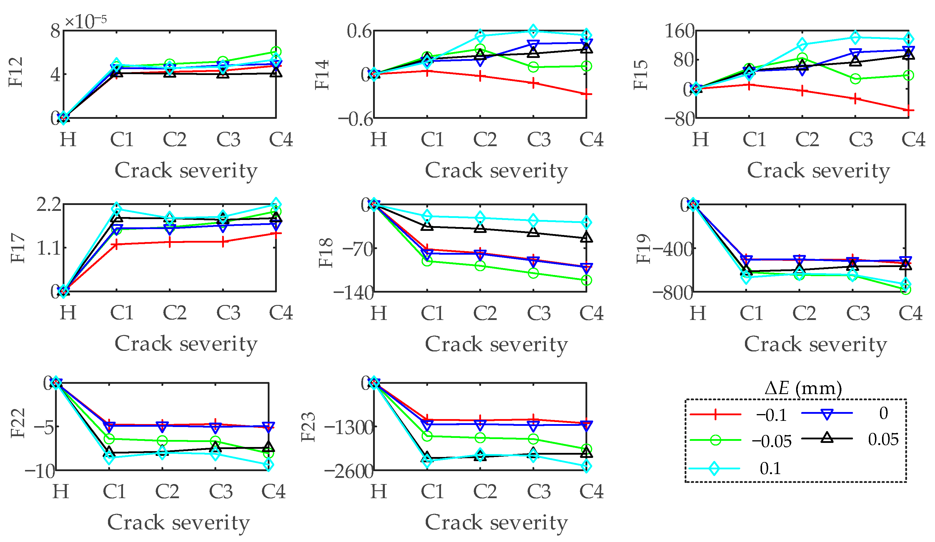
The system response is obtained by substituting the above TVMSs and the corresponding time-varying NLTE into the proposed dynamic model. It is already known that six time-domain indicators and eight frequency-domain indicators are sensitive to the tooth root crack fault of SBGP under the assembly error-free condition. They are A, P, SMR, C, I, and L in the time-domain, and F12, F14, F16, F17, F18, F19, F20, F21, F22 and F23 in the frequency-domain. Based on this, we will continue to analyze the sensitivity of these indicators to the SBGP tooth root crack fault under the influence of the offset error. According to the acceleration signal in the y direction of the bearing B3, the sensitivity of these indicators is obtained.
In Figure 23 and Figure 24, under the interference of offset error, the time-domain indicators A, P, C, I and L, and the frequency-domain indicators F12, F18 and F19 still maintain a good judgment threshold for fault information, so these indicators can be used as the indicators for diagnosing crack faults of the SBGP in the presence of offset error.
4. Conclusions
In this paper, the meshing model of the spiral bevel gear pair (SBGP) is established by the finite element (FE) method. The maximum tooth root stress value of the pinion and its position are studied considering the influence of assembly errors. The time-varying mesh stiffness (TVMS) of the SBGP under different degrees of tooth root crack fault of the pinion is derived. Meanwhile, the sensitivity of different statistical indicators to the crack fault of the pinion is verified by the dynamic simulation of the SBGP system. Through the analysis, some conclusions are summarized as follows:
- (1)
- Through static analysis, the value of the maximum tooth root stress and its position is discussed considering the assembly errors. It is found that the position of the maximum tooth root stress appears in the middle of the tooth width. The value is influenced by the assembly errors. To avoid excessive tooth root stress of the pinion, the changes in errors ΔE, ΔΣ and ΔAp should be strictly controlled. A smaller ΔE, ΔΣ, and a larger ΔAp are preferred to ease the pinion tooth root stress.
- (2)
- The dynamic response of the SBGP with the pinion tooth root crack fault is obtained by introducing the faulty TVMS curve as the excitation. When a crack fault occurs on the pinion, every time the pinion revolves one cycle, the faulty tooth participates in meshing for two meshing periods. There are fluctuations at intervals of the pinion rotation period in the time-domain waveform. Each time the faulty tooth participates in meshing, there are three meshing cycle mutations in the time-domain waveform. In the faulty amplitude spectrum, under the influence of the crack fault, sidebands with the rotation frequency of the pinion as the interval appear on both sides of the meshing frequency and its harmonics.
- (3)
- Through the analysis of statistical indicators. The sensitive indicators for identifying the root crack of the pinion are obtained. They are the A, P, SMR, C, I, and L in the time-domain, and F12, F14, F16, F17, F18, F19, F20, F21, F22 and F23 in the frequency-domain. These indicators can be used to monitor and diagnose crack faults in the SBGP system under the assembly error free condition. Moreover, under the interference of offset error, the time-domain indicators A, P, C, I and L, and the frequency-domain indicators F12, F18 and F19 still maintain a good judgment threshold for fault information, so these indicators can be used as the indicators for diagnosing crack faults in the presence of offset errors.
In the future, the research will focus on the simulation of the real tooth root crack fault morphology. The loaded tooth contact analysis will be carried out to solve the efficiency issues. Moreover, an experiment will be carried out in the future to validate the fault indicators for diagnosing the tooth root crack fault of SBGP.
Author Contributions
Conceptualization, H.H.; methodology, H.H.; software, H.H.; validation, H.H.; formal analysis, H.M.; investigation, H.H., H.W. and J.Z.; resources, H.M.; data curation, H.M.; writing—original draft preparation, H.H.; writing—review and editing, H.H., Z.L. (Zimeng Liu) and Z.L. (Zhanwei Li); visualization, H.H.; supervision, H.M.; project administration, H.M.; funding acquisition, H.M. All authors have read and agreed to the published version of the manuscript.
Funding
This research was funded by “Fundamental Research Funds for the Central Universities, grant number N2103024”, the “National Science and Technology Major Project, grant number J2019-IV-0018-0086”, the “National Key Laboratory of Science and Technology on Helicopter Transmission”, grant number HTL-O-21G03”.
Institutional Review Board Statement
Not applicable.
Informed Consent Statement
Not applicable.
Data Availability Statement
Not applicable.
Conflicts of Interest
The authors declare no conflict of interest.
Appendix A
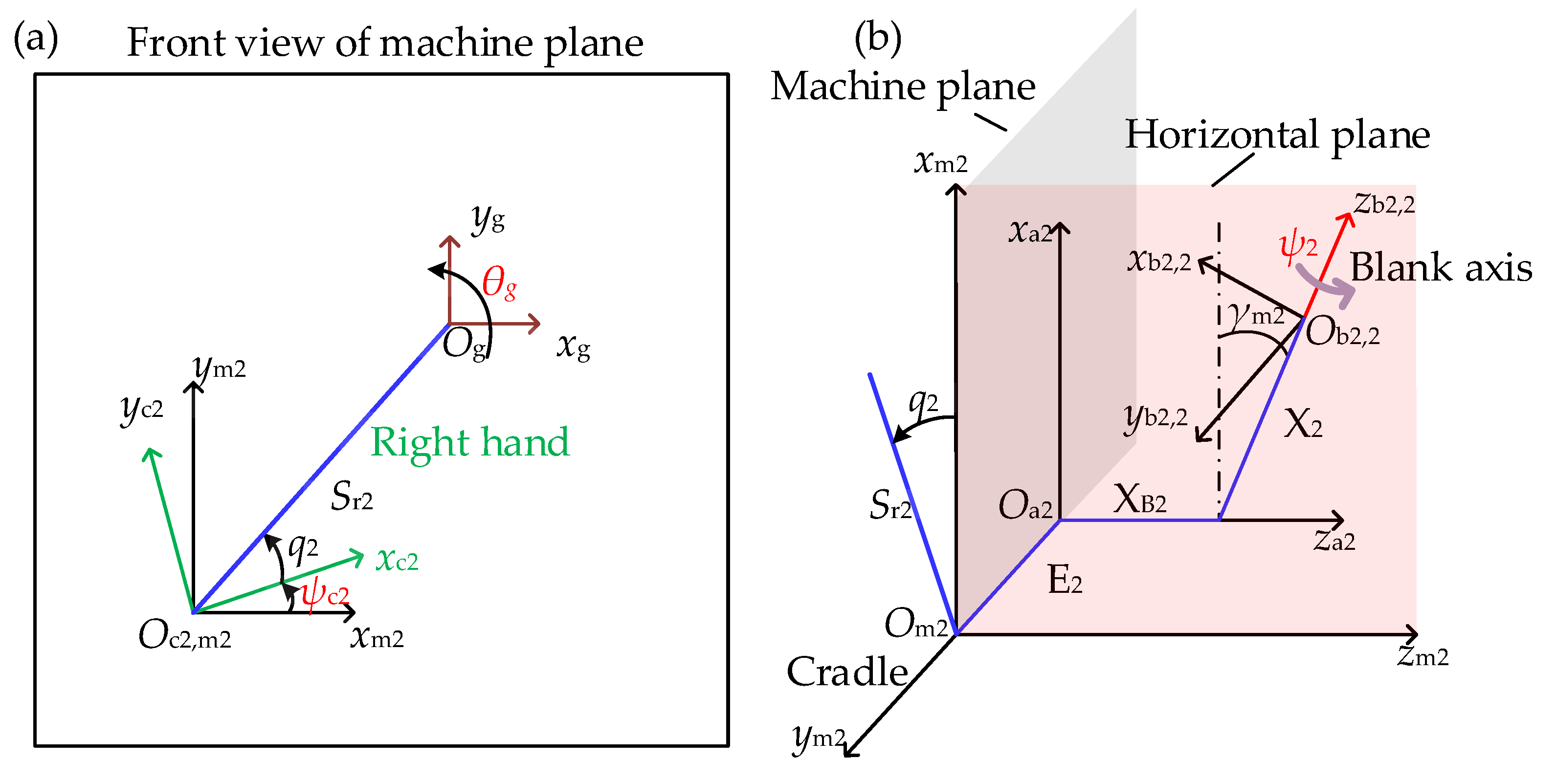
The machine tool coordinate for machining bevel gear by the generating method is illustrated in Figure A1; any point of the cutter in the cutter coordinate system Og-xg-yg-zg can be expressed in the blank coordinate system through the following coordinate transformation:
where θg is the rotation angle of the cutter; Sr2 is radial distance; q2 is the cradle angle; XB2 is the sliding base; E2 is the blank offset; γm2 is the machine root angle; X2 is the machine center to back; ψ2 is the blank rotation angle; ψc2 is the cradle rotation angle; and ψc2 = ψ2/i2, i2 is the velocity ratio. The detail of the coordinate transformation matrix ROTY(θ), ROTZ(θ), TRNX(δ), TRNY(δ), and TRNZ(δ) are expressed as:
Figure A1.
The layout of the machine tool coordinate for machining bevel gear by the generating method: (a) Front view; (b) General view.
Figure A1.
The layout of the machine tool coordinate for machining bevel gear by the generating method: (a) Front view; (b) General view.
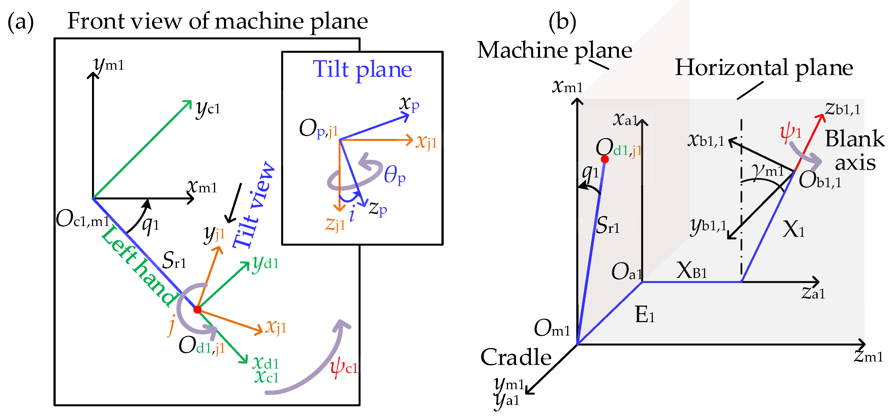
The machine tool coordinate for machining bevel pinion by the tilt method is illustrated in Figure A2; any point of the cutter in the cutter coordinate system Op-xp-yp-zp can be expressed in the blank coordinate system through the following coordinate transformation:
where θp is the rotation angle of the cutter; i is the tilt angle; j is the swivel angle; Sr1 is radial distance; q1 is the cradle angle; XB1 is the sliding base; E1 is the blank offset; γm1 is the machine root angle; X1 is the machine center to back; ψ1 is the blank rotation angle; ψc1 is the cradle rotation angle; and ψc1 = ψ1/i1, i1 is the velocity ratio.
Figure A2.
The layout of the machine tool coordinate for machining bevel pinion by the tilt method: (a) Front view; (b) General view.
Figure A2.
The layout of the machine tool coordinate for machining bevel pinion by the tilt method: (a) Front view; (b) General view.
The schematic of the cutter is illustrated in Figure A3. The inner blade (IB) mills the convex side of the gear, and the outer blade (OB) mills the concave side of the blade.
Figure A3.
Schematic of the cutter.

In the coordinate of the cutter Oi-xi-yi-zi, (i = p, g denotes cutter machining the bevel pinion and the bevel gear, respectively), the flank and the transition zone can be expressed by:
where j = I, O represents the inner blade and the outer blade, respectively; τi is the distance from the tooth flank to the tooth tip; the “±” corresponds to the concave side and the convex side, respectively; γj is the central angle between any point on the transition arc and T0j, where T0j is the point of tangent between the tooth surface and the transition zone. When machining the concave surface of the gear, the value range of γj is [0, π/2 + α0j], and when machining the convex surface of the gear, the value range of γj is [−π/2 + α0j, 0].
In the coordinate of the blank Oi-xi-yi-zi, (i = 1, 2 denotes the blank of the bevel pinion and the bevel gear, respectively), the tooth surface equation can be expressed as:
When machining the bevel gear, the tooth surface coordinate r2 satisfies the following relation:
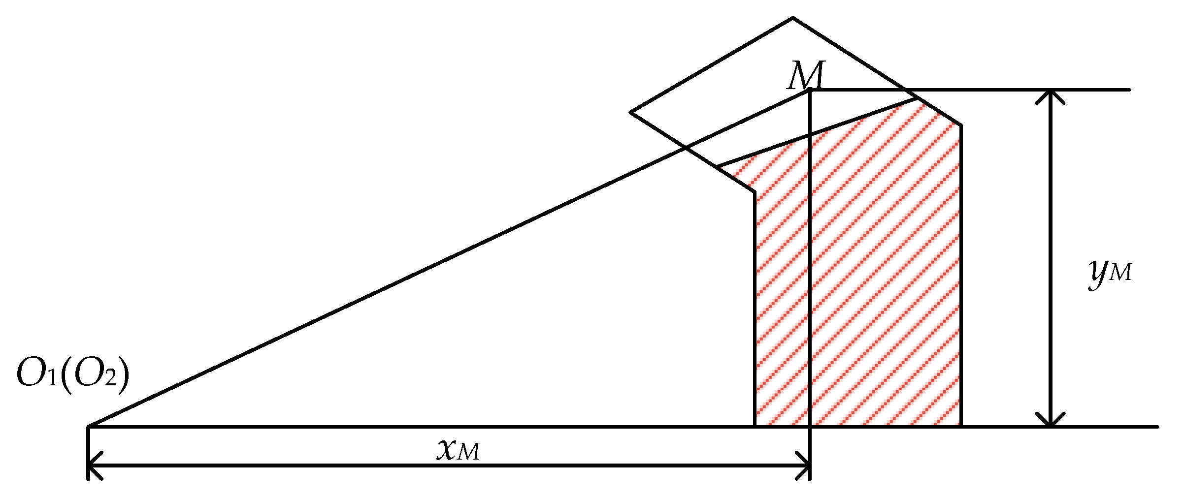
On the gear rotation projection surface, the coordinate M (xM, yM) of any point (see Figure A4) satisfies the following equations:
Figure A4.
Tooth face point in the rotation projection plane.
Combining Equations (A6) and (A7), the spatial position of any surface point can be obtained.
When machining the bevel pinion, in the coordinate of the machine Om1-xm1-ym1-zm1, the position of the cutter can be expressed as:
In the process of machining the bevel pinion by the tilt method, the tooth surface coordinate rm1 satisfies the following relation:
where the direction of the tooth surface point in the coordinate of the machine can be expressed as:
The relative rotation vector can be expressed as:
where,
On the pinion rotation projection surface, the coordinate M (xM, yM) of any point (see Figure A4) satisfies the following equations:
Combining Equations (A10) and (A13), the spatial position of any surface point can be obtained.
References
- Kim, D.H.; Kim, J.H.; Kim, G.G.; Lee, Y.S. Random fatigue analysis of automotive bevel gear. Key Eng. Mater. 2006, 326–328, 987–990. [Google Scholar] [CrossRef]
- Park, M. Failure analysis of an accessory bevel gear installed on a J69 turbojet engine. Eng. Fail. Anal. 2003, 10, 371–382. [Google Scholar] [CrossRef]
- Spievak, L.E.; Wawrzynek, P.A.; Ingraffea, A.R.; Lewicki, D.G. Simulating fatigue crack growth in spiral bevel gears. Eng. Fract. Mech. 2001, 68, 53–76. [Google Scholar] [CrossRef] [Green Version]
- Lewicki, D.G.; Handschuh, R.F.; Spievak, L.E.; Wawrzynek, P.A.; Ingraffea, A.R. Consideration of moving tooth load in gear crack propagation predictions. J. Mech. Des. 2000, 123, 118–124. [Google Scholar] [CrossRef]
- Vukelic, G.; Pastorcic, D.; Vizentin, G.; Bozic, Z. Failure investigation of a crane gear damage. Eng. Fail. Anal. 2020, 115, 104613. [Google Scholar] [CrossRef]
- Ural, A.; Heber, G.; Wawrzynek, P.A.; Ingraffea, A.R.; Lewicki, D.G.; Neto, J.B.C. Three-dimensional, parallel, finite element simulation of fatigue crack growth in a spiral bevel pinion gear. Eng. Fract. Mech. 2005, 72, 1148–1170. [Google Scholar] [CrossRef]
- Böhme, S.A.; Vinogradov, A.; Papuga, J.; Berto, F. A novel predictive model for multiaxial fatigue in carburized bevel gears. Fatigue Fract. Eng. Mater. Struct. 2021, 44, 2033–2053. [Google Scholar] [CrossRef]
- Ma, H.; Zeng, J.; Feng, R.; Pang, X.; Wen, B. An improved analytical method for mesh stiffness calculation of spur gears with tip relief. Mech. Mach. Theory 2016, 98, 64–80. [Google Scholar] [CrossRef]
- Zhao, Z.; Yang, Y.; Han, H.; Ma, H.; Wang, H.; Li, Z. Meshing Characteristics of Spur Gears Considering Three-Dimensional Fractal Rough Surface under Elastohydrodynamic Lubrication. Machines 2022, 10, 705. [Google Scholar] [CrossRef]
- Chen, K.; Huangfu, Y.; Ma, H.; Xu, Z.; Li, X.; Wen, B. Calculation of mesh stiffness of spur gears considering complex foundation types and crack propagation paths. Mech. Syst. Signal Process. 2019, 130, 273–292. [Google Scholar] [CrossRef]
- Huangfu, Y.; Chen, K.; Ma, H.; Li, X.; Han, H.; Zhao, Z. Meshing and dynamic characteristics analysis of spalled gear systems: A theoretical and experimental study. Mech. Syst. Signal Process. 2020, 139, 106640. [Google Scholar] [CrossRef]
- Liu, Z.; Huangfu, Y.; Ma, H.; Peng, Z.; Zhu, J.; Wang, H.; Li, Z. Traveling wave resonance analysis of flexible spur gear system with angular misalignment. Int. J. Mech. Sci. 2022, 232, 107617. [Google Scholar] [CrossRef]
- Zhao, Z.; Han, H.; Wang, P.; Ma, H.; Zhang, S.; Yang, Y. An improved model for meshing characteristics analysis of spur gears considering fractal surface contact and friction. Mech. Mach. Theory 2021, 158, 104219. [Google Scholar] [CrossRef]
- Mu, Y.; Li, W.; Fang, Z.; Zhang, X. A novel tooth surface modification method for spiral bevel gears with higher-order transmission error. Mech. Mach. Theory 2018, 126, 49–60. [Google Scholar] [CrossRef]
- Mu, Y.; He, X. Design and dynamic performance analysis of high-contact-ratio spiral bevel gear based on the higher-order tooth surface modification. Mech. Mach. Theory 2021, 161, 104312. [Google Scholar] [CrossRef]
- Ding, H.; Tang, J.; Zhou, Y.; Zhong, J.; Wan, G. A multi-objective correction of machine settings considering loaded tooth contact performance in spiral bevel gears by nonlinear interval number optimization. Mech. Mach. Theory 2017, 113, 85–108. [Google Scholar] [CrossRef]
- Ding, H.; Tang, J.; Zhong, J. An accurate model of high-performance manufacturing spiral bevel and hypoid gears based on machine setting modification. J. Manuf. Syst. 2016, 41, 111–119. [Google Scholar] [CrossRef]
- Kolivand, M.; Kahraman, A. An ease-off based method for loaded tooth contact analysis of hypoid gears having local and global surface deviations. J. Mech. Des. 2009, 132, 245–254. [Google Scholar]
- Hu, Z.; Ding, H.; Peng, S.; Tang, Y.; Tang, J. Numerical determination to loaded tooth contact performances in consideration of misalignment for the spiral bevel gears. Int. J. Mech. Sci. 2019, 151, 343–355. [Google Scholar] [CrossRef]
- Peng, S.; Ding, H.; Zhang, G.; Tang, J.; Tang, Y. New determination to loaded transmission error of the spiral bevel gear considering multiple elastic deformation evaluations under different bearing supports. Mech. Mach. Theory 2019, 137, 37–52. [Google Scholar] [CrossRef]
- Bibel, G.D.; Kumar, A.; Reddy, S.; Handschuh, R. Contact stress analysis of spiral bevel gears using finite element analysis. J. Mech. Des. 1995, 117, 235–240. [Google Scholar] [CrossRef]
- Argyris, J.; Fuentes, A.; Litvin, F.L. Computerized integrated approach for design and stress analysis of spiral bevel gears. Comput. Methods Appl. Mech. Eng. 2002, 191, 1057–1095. [Google Scholar] [CrossRef]
- Gonzalez-Perez, I.; Fuentes-Aznar, A. Reverse engineering of spiral bevel gear drives reconstructed from point clouds. Mech. Mach. Theory 2022, 170, 104694. [Google Scholar] [CrossRef]
- Hou, X.; Fang, Z.; Zhang, X. Static contact analysis of spiral bevel gear based on modified VFIFE (vector form intrinsic finite element) method. Appl. Math. Model. 2018, 60, 192–207. [Google Scholar] [CrossRef]
- Gan, L.; Xiao, K.; Wang, J.; Pu, W.; Cao, W. A numerical method to investigate the temperature behavior of spiral bevel gears under mixed lubrication condition. Appl. Ther. Eng. 2019, 147, 866–875. [Google Scholar] [CrossRef]
- Fu, Y.; Zhuo, Y.; Zhou, X.; Wan, B.; Lv, H.; Wang, Z. Theoretical and experimental study on contact characteristics of spiral bevel gears under quasi-static and large loading conditions. Appl. Sci. 2020, 10, 5109. [Google Scholar] [CrossRef]
- Hou, X.; Fang, Z.; Fu, X.; Zhang, X. Meshing performance of spiral bevel gear with different loads and modules considering edge contact by finite element method. Trans. Can. Soc. Mech. Eng. 2019, 43, 322–332. [Google Scholar] [CrossRef]
- Wang, P.-Y.; Fan, S.-C.; Huang, Z.-G. Spiral bevel gear dynamic contact and tooth impact analysis. J. Mech. Des. 2011, 133, 084501. [Google Scholar] [CrossRef]
- Guo, W.; Mao, S.; Yang, Y.; Kuang, Y. Optimization of cutter blade profile for face-hobbed spiral bevel gears. Int. J. Adv. Manuf. Technol. 2015, 85, 209–216. [Google Scholar] [CrossRef]
- Wang, Y.; Tang, W.; Chen, Y.; Wang, T.; Li, G.; Ball, A.D. Investigation into the meshing friction heat generation and transient thermal characteristics of spiral bevel gears. Appl. Ther. Eng. 2017, 119, 245–253. [Google Scholar] [CrossRef]
- Yang, D.; Chen, L.; Jiang, L.; Wang, P.; Tao, J. Research on the influence of time-varying excitation on vibration characteristics of the spiral bevel geared transmission system with broken teeth. Shock Vib. 2021, 2021, 8880851. [Google Scholar] [CrossRef]
- Ding, H.; Tang, J.; Zhong, J.; Zhou, Z. A hybrid modification approach of machine-tool setting considering high tooth contact performance in spiral bevel and hypoid gears. J. Manuf. Syst. 2016, 41, 228–238. [Google Scholar] [CrossRef]
- Litvin, F.L.; Fuentes, A. Gear Geometry and Applied Theory; Cambridge University Press: Cambridge, UK, 2004. [Google Scholar]
- Han, H.; Zhang, S.; Yang, Y.; Ma, H.; Jiang, L. Modulation sidebands analysis of coupled bevel gear pair and planetary gear train system. Mech. Mach. Theory 2022, 176, 104979. [Google Scholar] [CrossRef]
- Tayyab, S.M.; Chatterton, S.; Pennacchi, P. Fault Detection and Severity Level Identification of Spiral Bevel Gears under Different Operating Conditions Using Artificial Intelligence Techniques. Machines 2021, 9, 173. [Google Scholar] [CrossRef]

Figure 2.
Example of assembly error of SBGP.
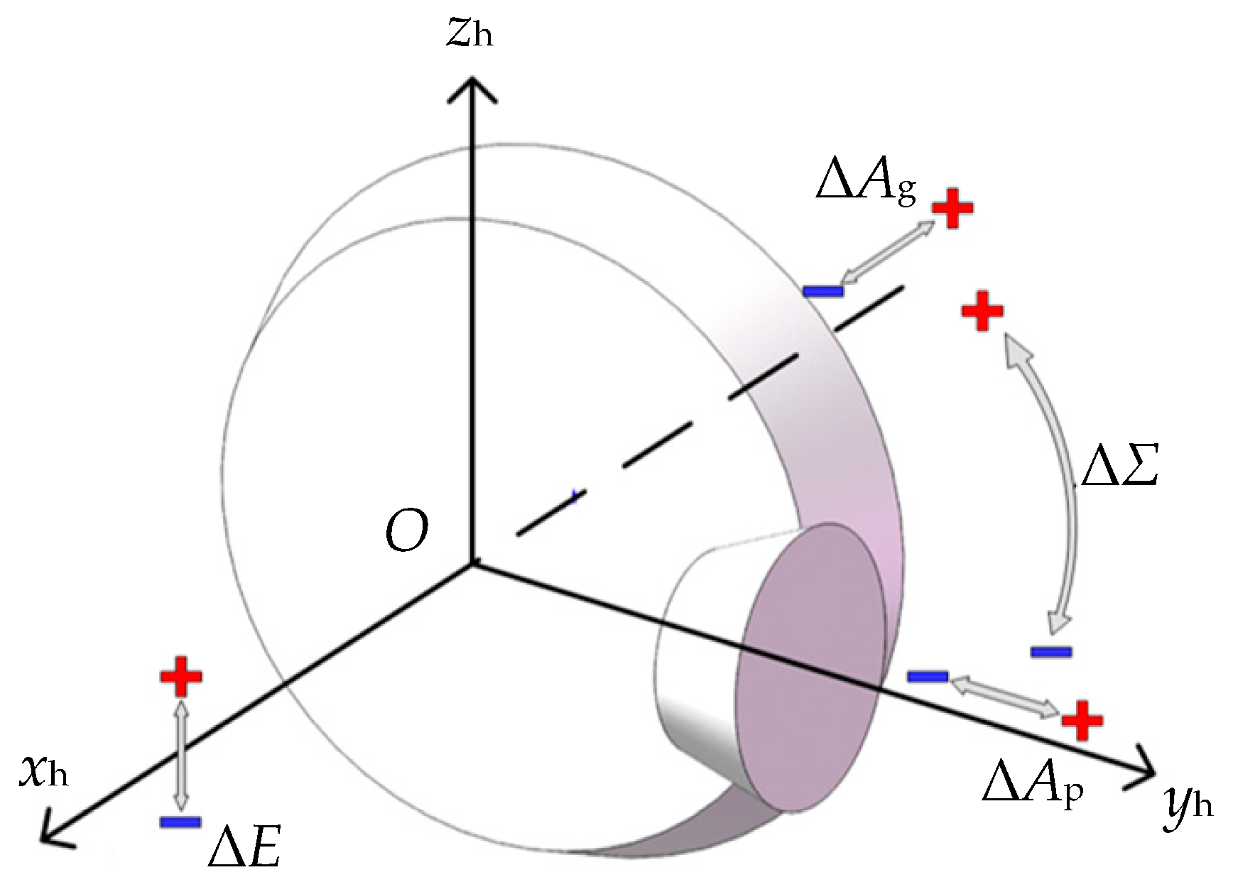
Figure 3.
Contact trajectories and NLTEs variation due to the assembly errors: (a) ΔE; (b) ΔΣ; (c) ΔAg; (d) ΔAp.
Figure 3.
Contact trajectories and NLTEs variation due to the assembly errors: (a) ΔE; (b) ΔΣ; (c) ΔAg; (d) ΔAp.
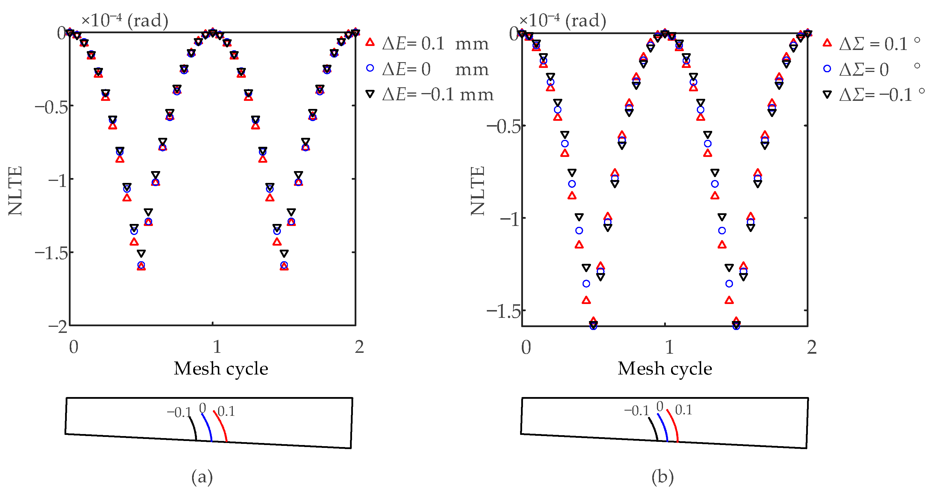
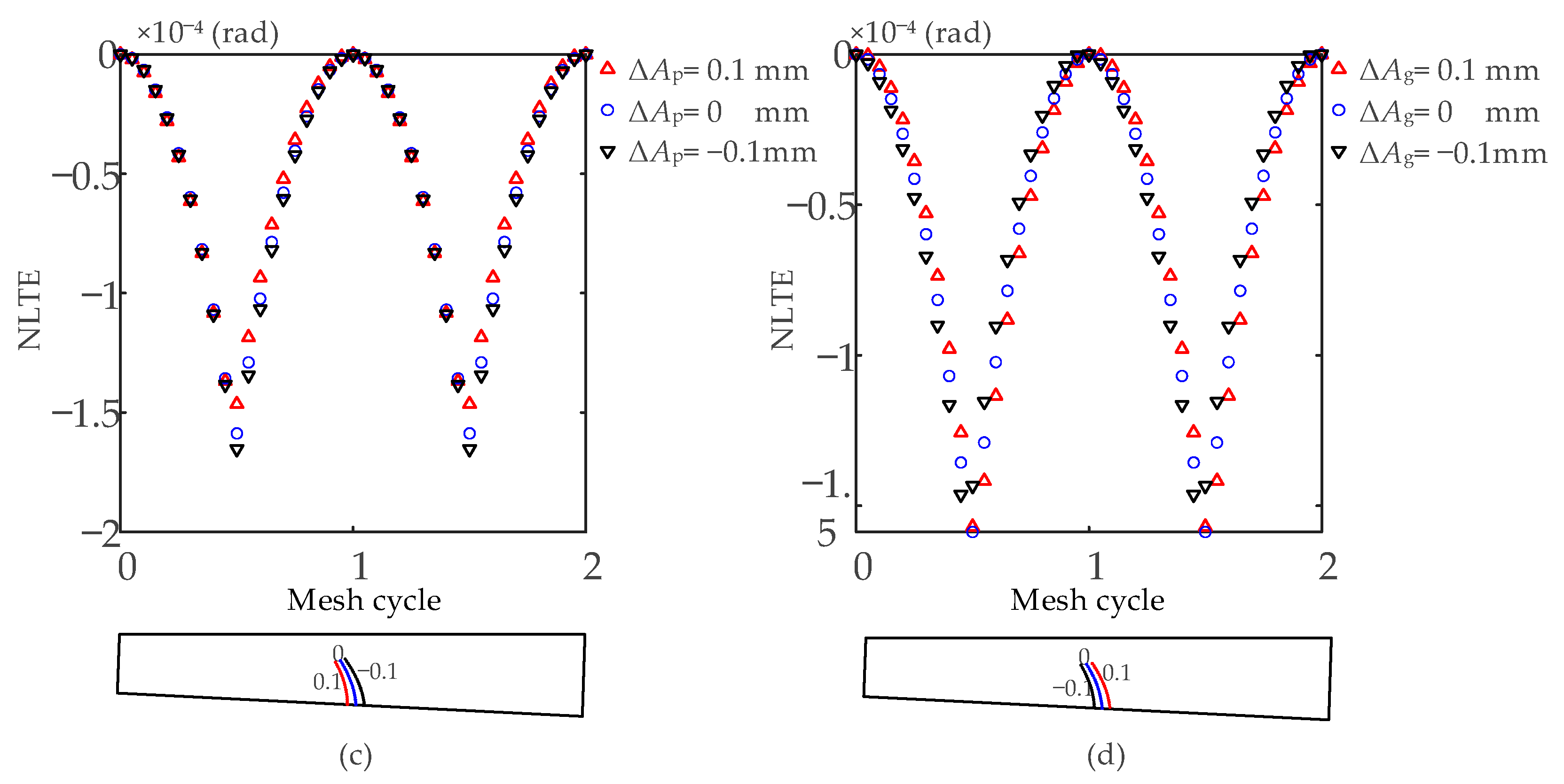
Figure 4.
FE model of the SBGP.

Figure 5.
TVMS of the SBGP in a healthy state.
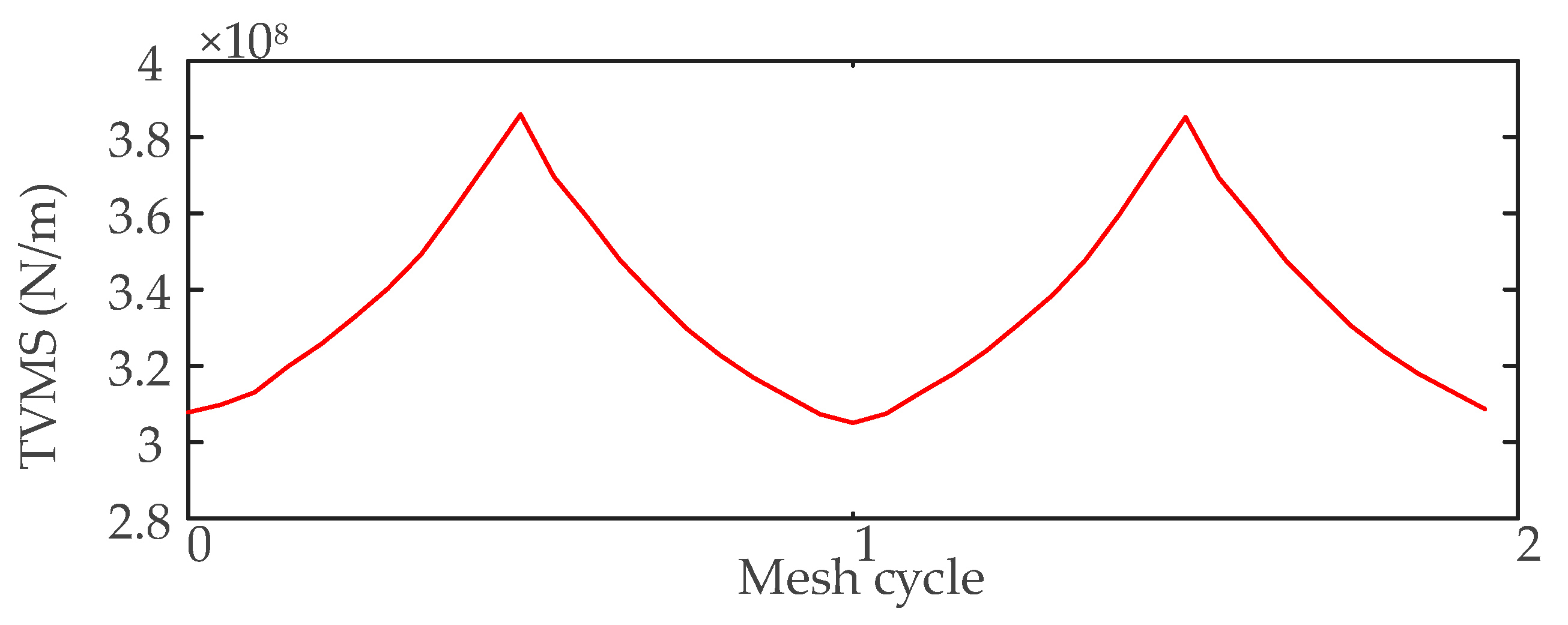
Figure 6.
Bevel pinion crack propagation path [6].
Figure 6.
Bevel pinion crack propagation path [6].
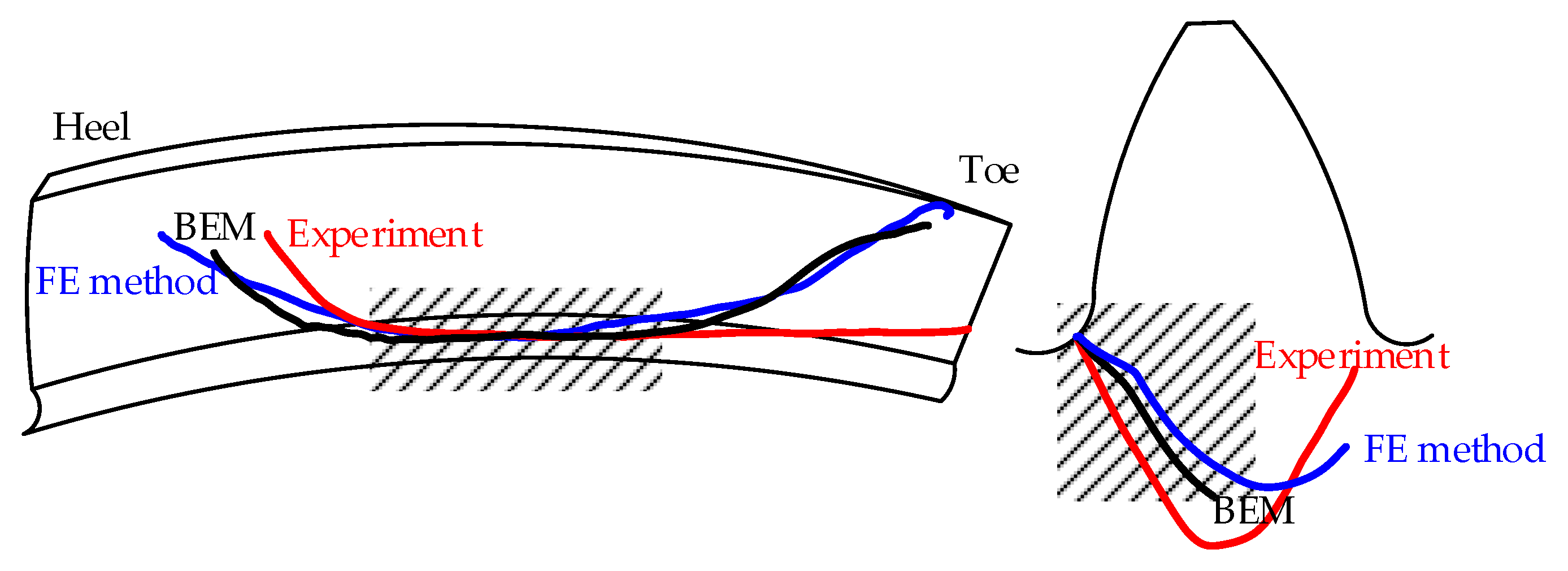
Figure 7.
Node replacement method to generate crack section: (a) Node replacement example; (b) Crack characterization parameters.
Figure 7.
Node replacement method to generate crack section: (a) Node replacement example; (b) Crack characterization parameters.
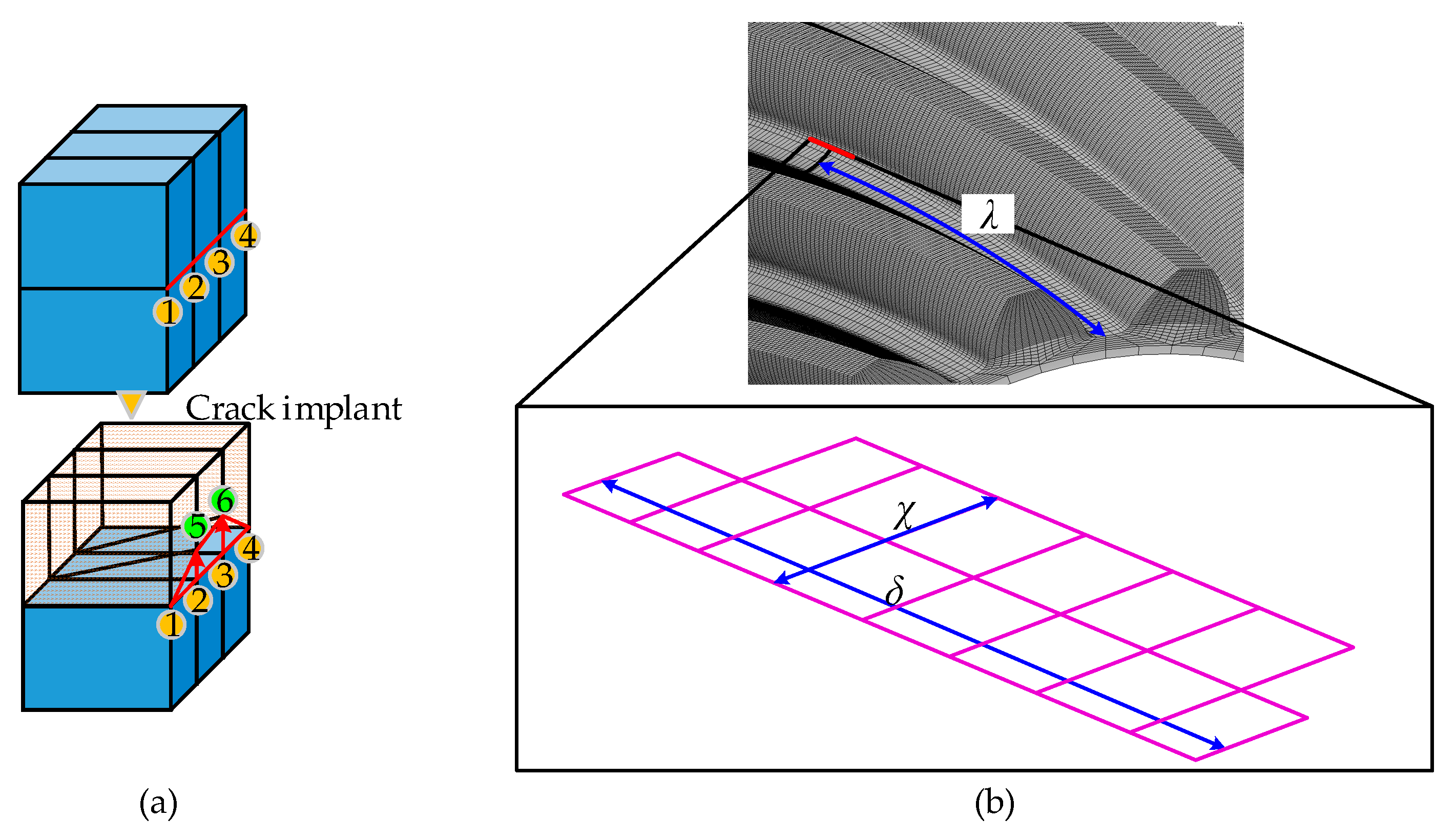
Figure 8.
Flow chart of the FE modelling process.

Figure 9.
Contour plot of the von Mises stress distribution of the pinion: (a) 3D view; (b) Plane view.
Figure 9.
Contour plot of the von Mises stress distribution of the pinion: (a) 3D view; (b) Plane view.
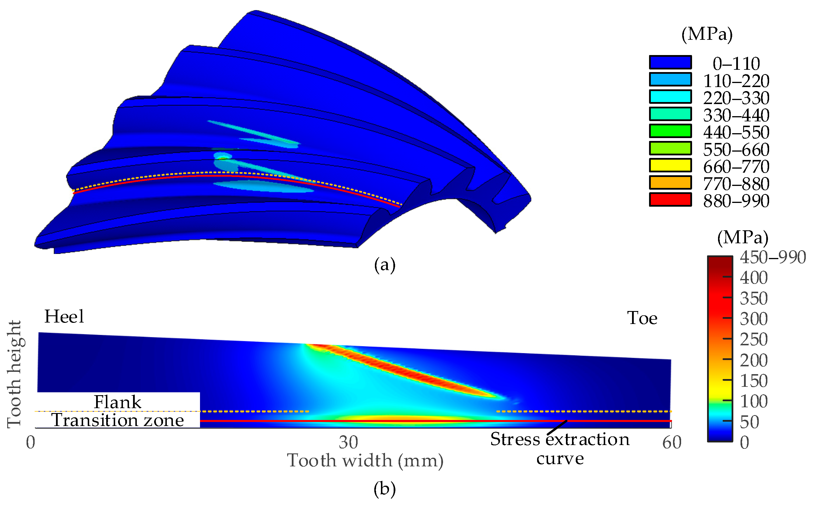
Figure 10.
Variation of tooth root stress in three mesh cycles considering the variation of offset error.
Figure 10.
Variation of tooth root stress in three mesh cycles considering the variation of offset error.

Figure 11.
Variation of tooth root stress in three mesh cycles considering the variation of shaft angle error.
Figure 11.
Variation of tooth root stress in three mesh cycles considering the variation of shaft angle error.
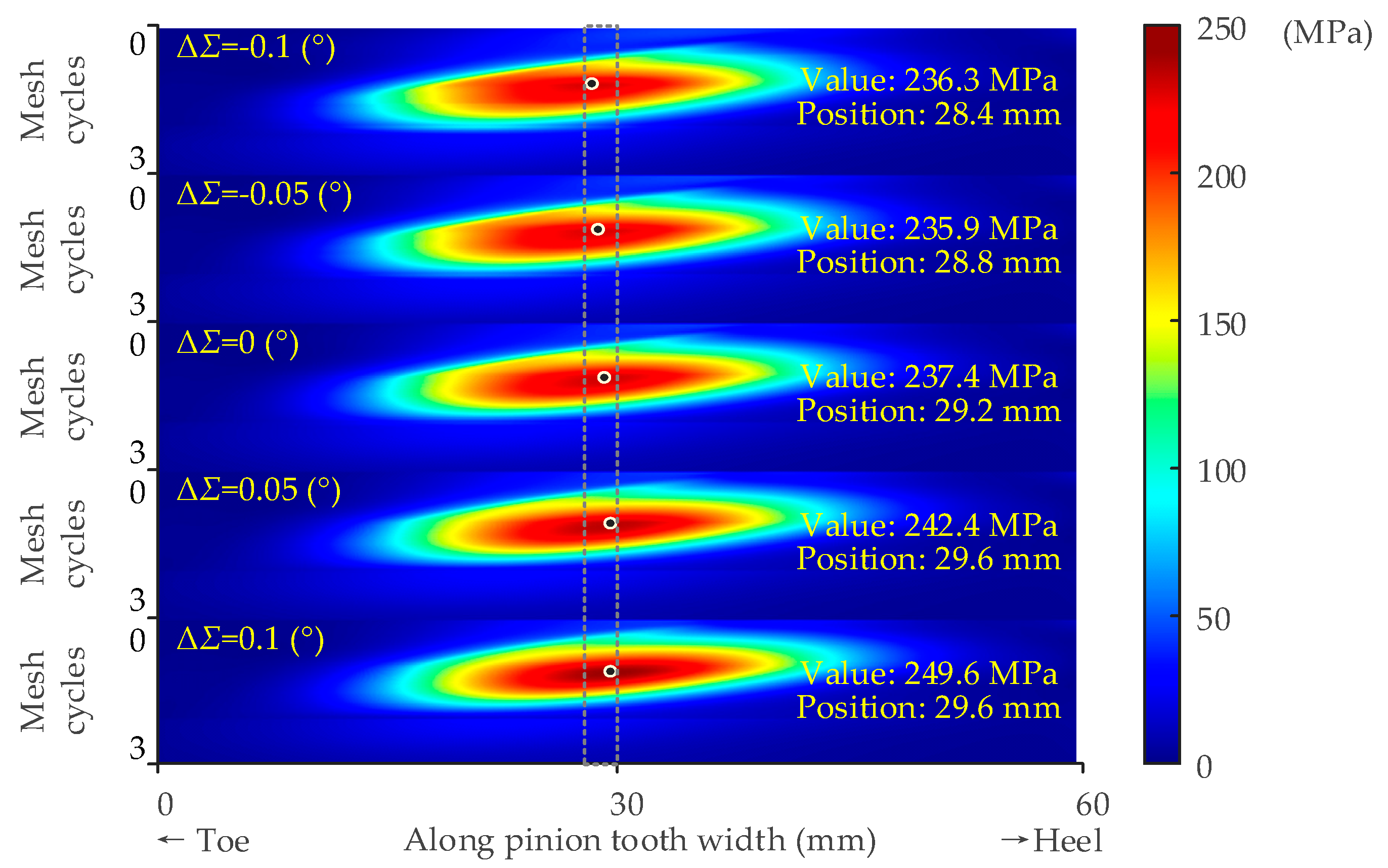
Figure 12.
Variation of tooth root stress in three mesh cycles considering the variation of pinion axial error.
Figure 12.
Variation of tooth root stress in three mesh cycles considering the variation of pinion axial error.
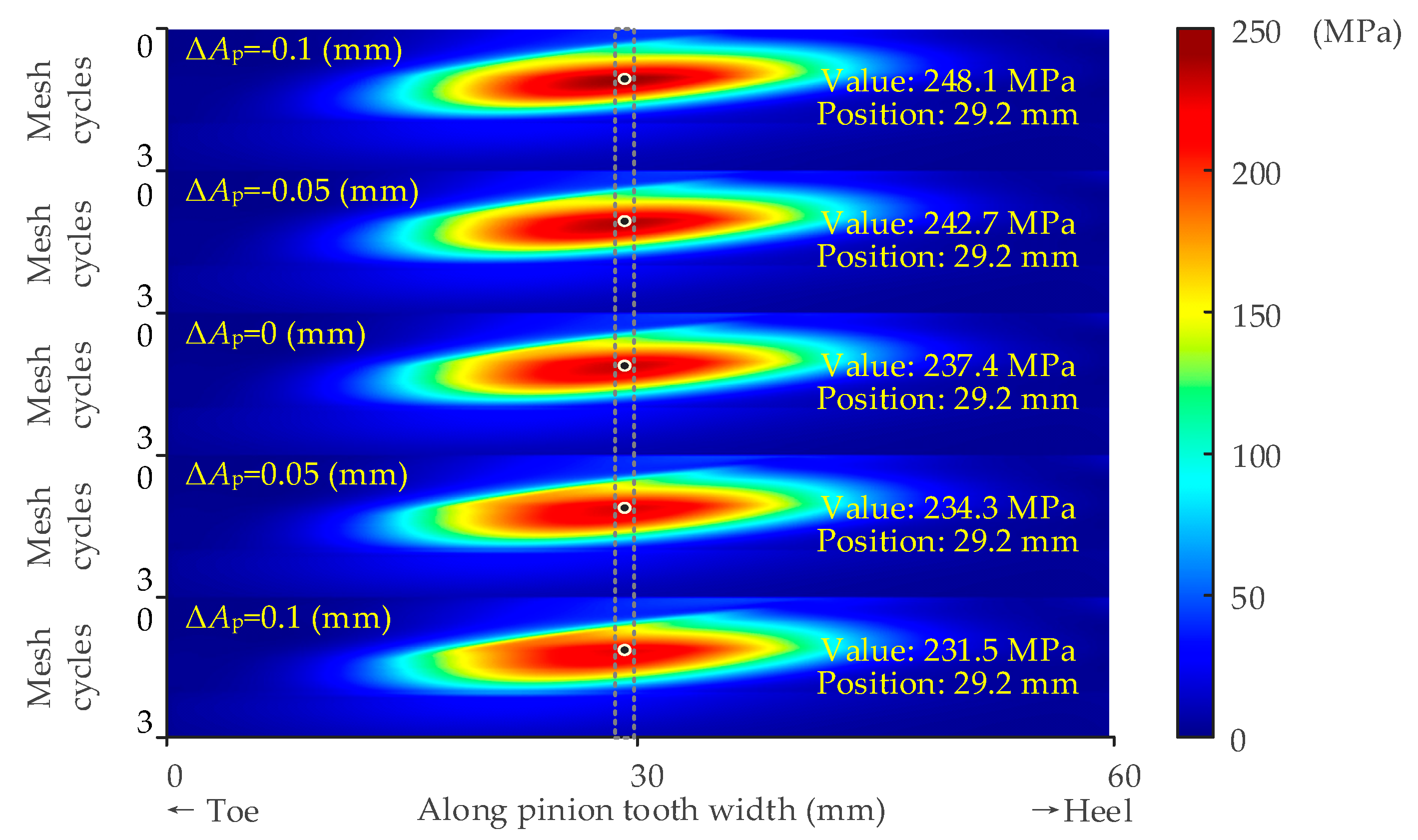
Figure 13.
Variation of tooth root stress in three mesh cycles considering the variation of gear axial error.
Figure 13.
Variation of tooth root stress in three mesh cycles considering the variation of gear axial error.

Figure 14.
Cross-section morphology of the simulated cracks.

Figure 15.
TVMS and the initial gaps of the SBGP: (a) TVMS versus different crack levels; (b) The initial gaps during two meshing cycles.
Figure 15.
TVMS and the initial gaps of the SBGP: (a) TVMS versus different crack levels; (b) The initial gaps during two meshing cycles.
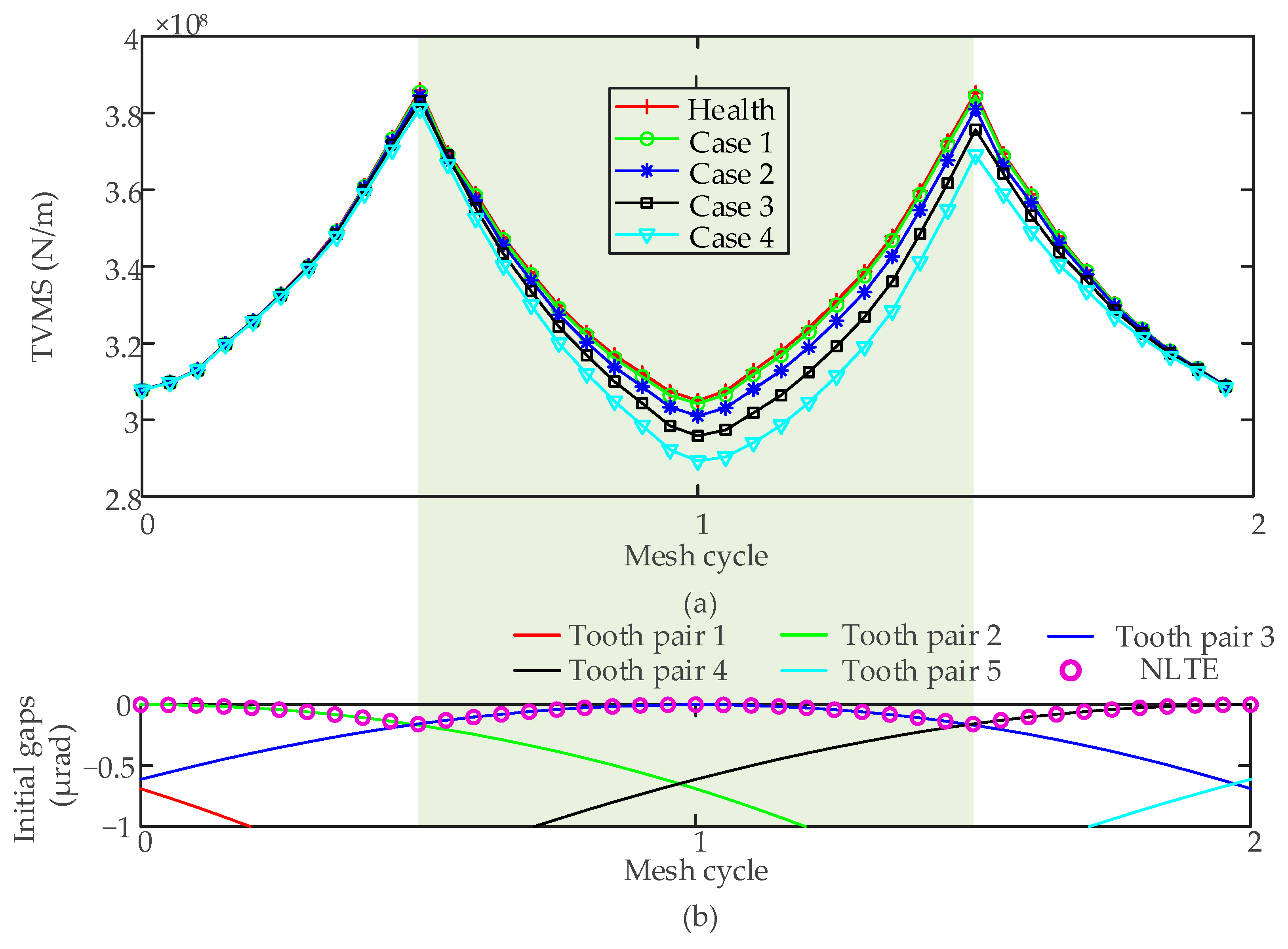
Figure 16.
A schematic of the coupling SBGP and shafts system.
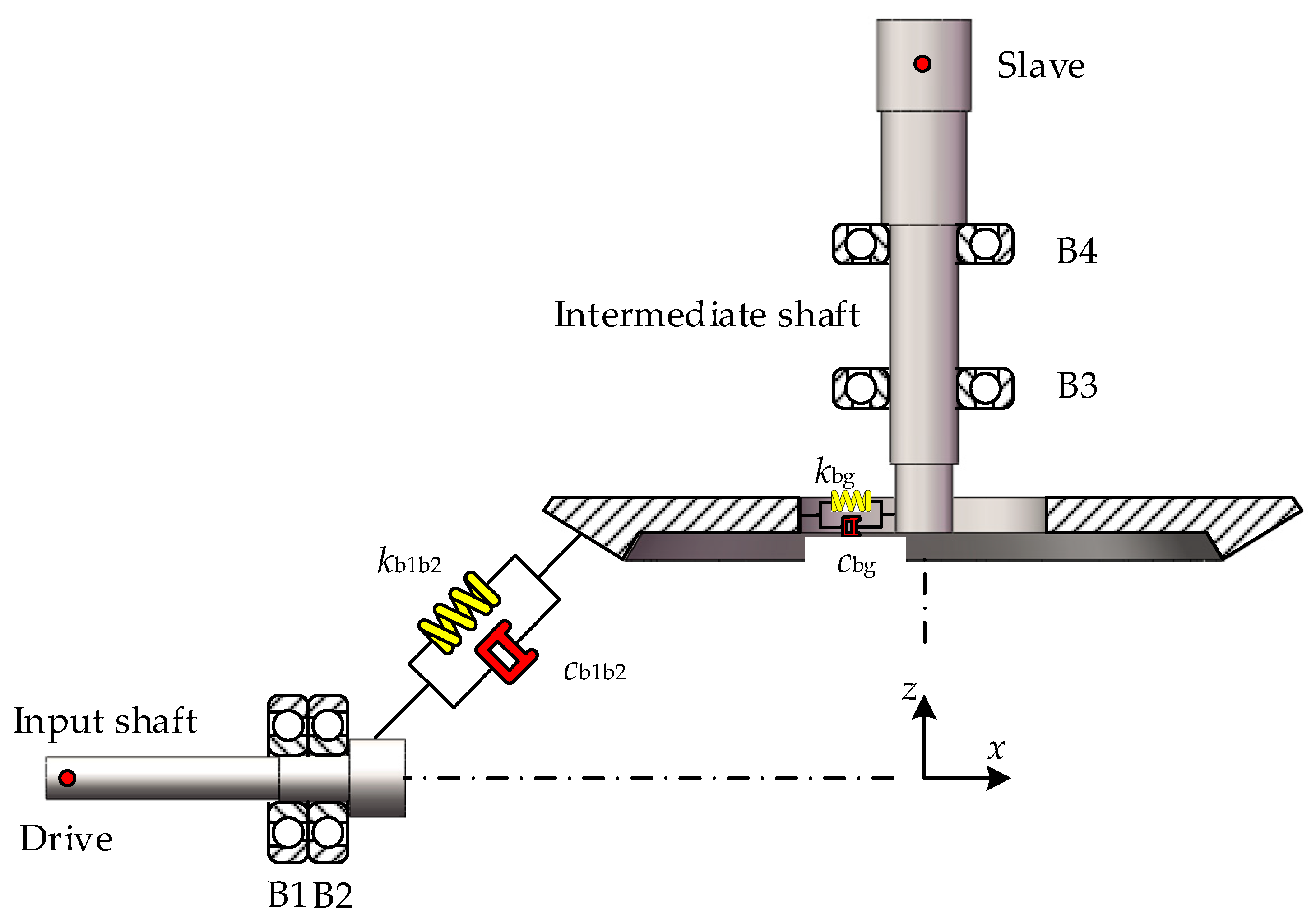
Figure 17.
The schematic of the grouping of the system stiffness matrix and damping matrix.
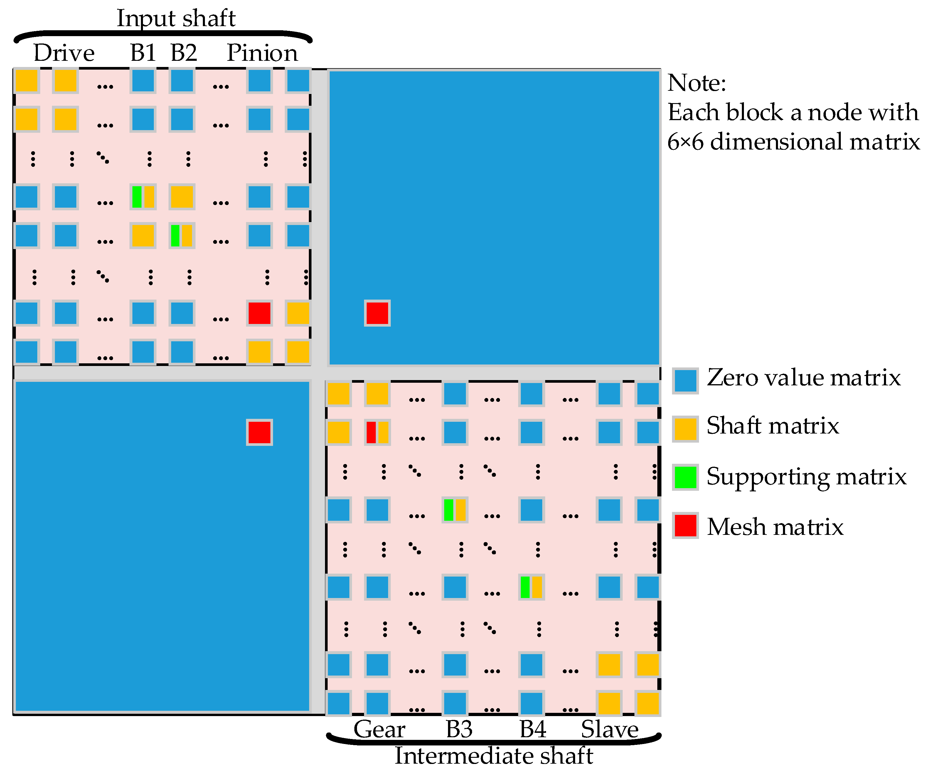
Figure 18.
Health condition: (a) Time-domain waveform; (b) Amplitude spectrum.
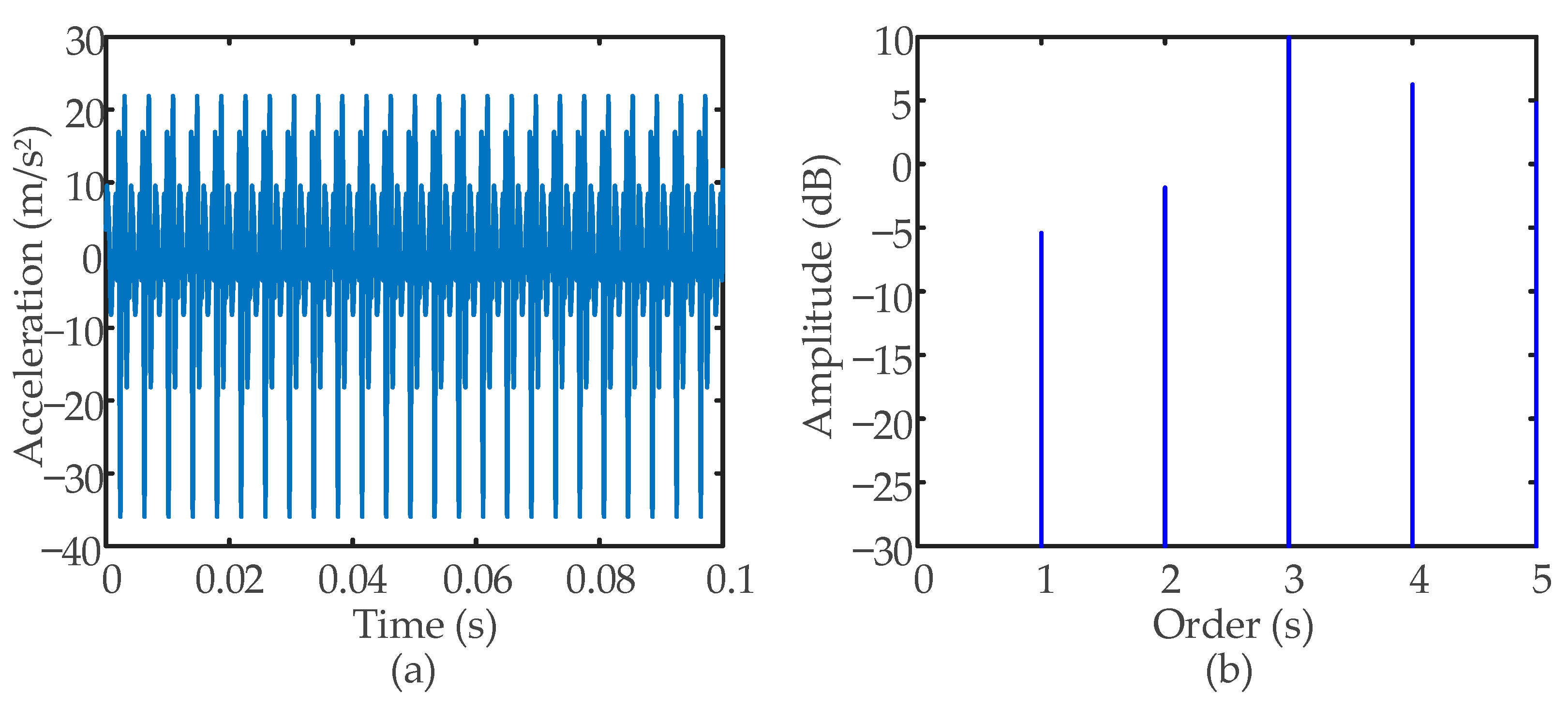
Figure 19.
Case 4: (a) Time-domain waveform; (b) Amplitude spectrum.
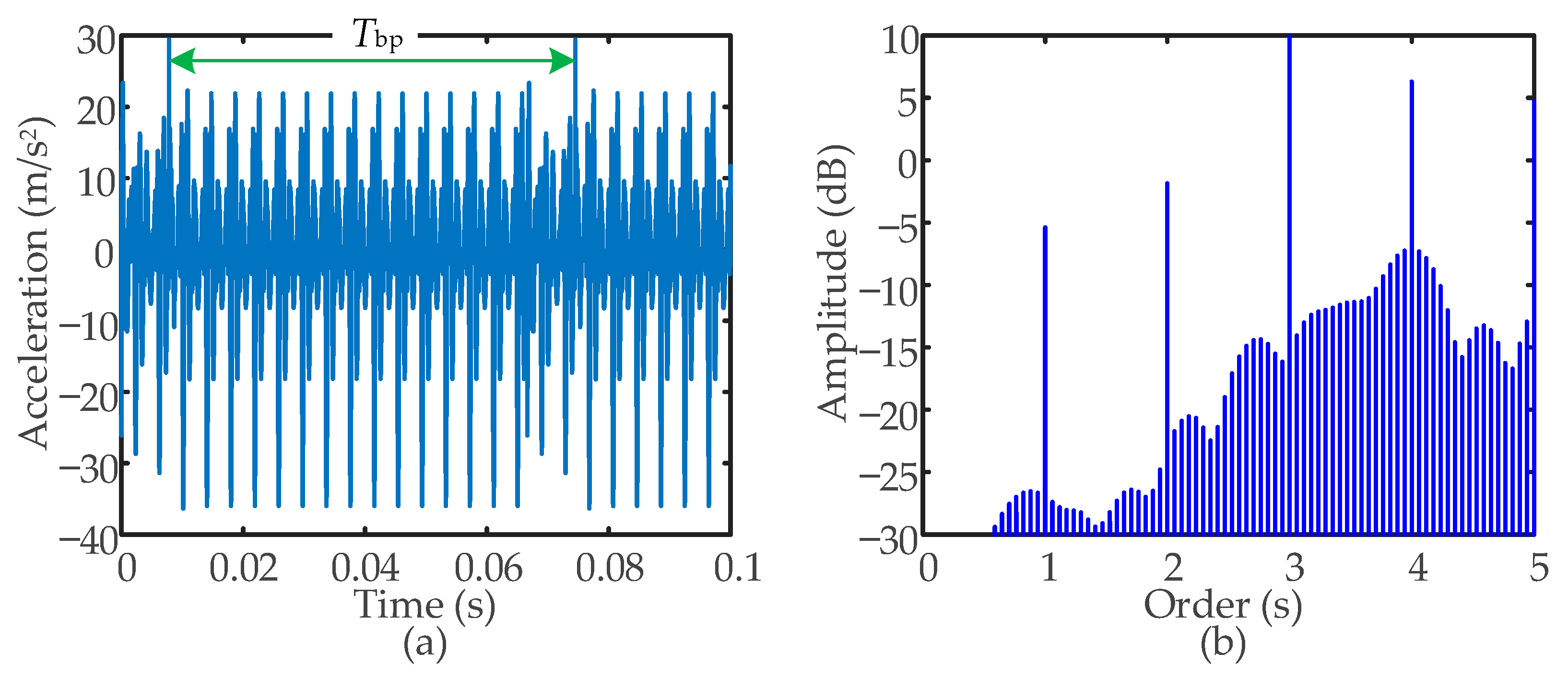
Figure 20.
Fluctuations of time-domain indicators relative to the healthy condition for different crack degrees.
Figure 20.
Fluctuations of time-domain indicators relative to the healthy condition for different crack degrees.
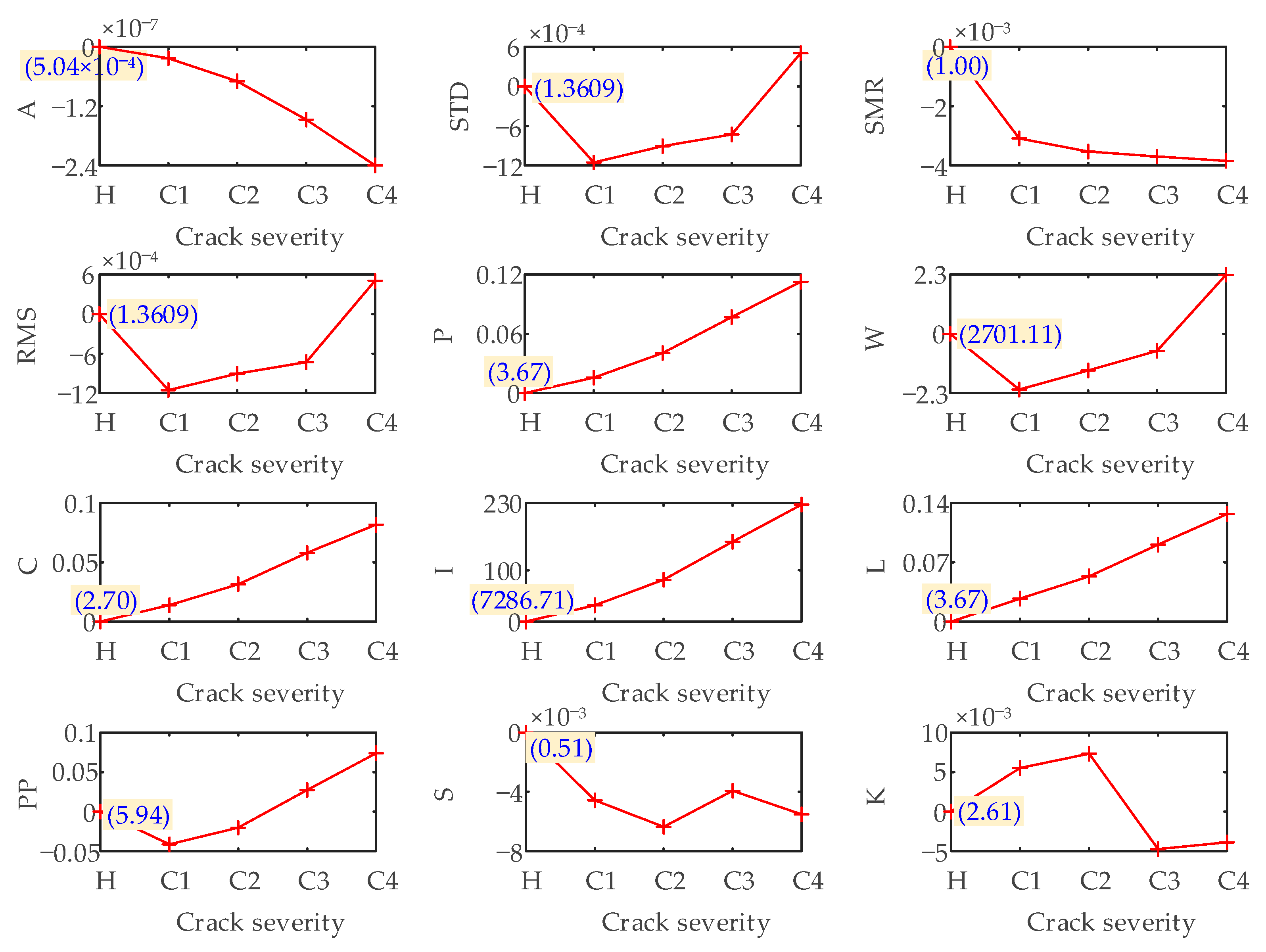
Figure 21.
Fluctuations of frequency-domain indicators relative to the healthy condition for different crack degrees.
Figure 21.
Fluctuations of frequency-domain indicators relative to the healthy condition for different crack degrees.
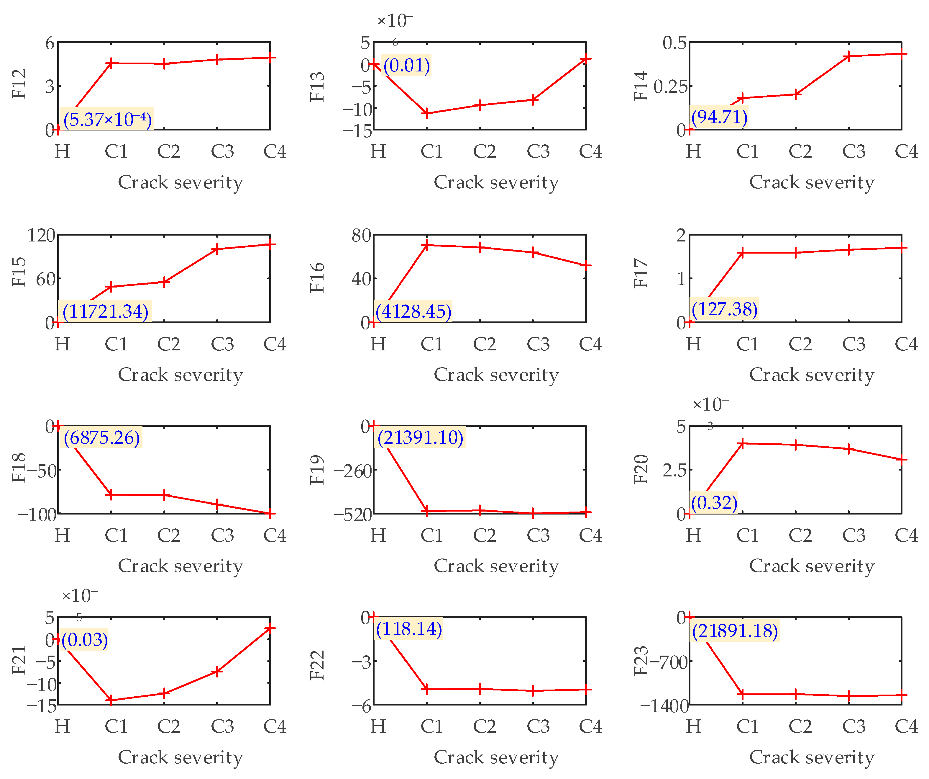
Figure 22.
TVMS curves of SBGP considering assembly errors and crack faults: (a) TVMS in health conditions with offset errors; (b) TVMS curves in the condition of ΔE = −0.1 mm with different crack degrees; (c) TVMS curves in the condition of ΔE = −0.05 mm with different crack degrees; (d) TVMS curves in the condition of ΔE = 0 mm with different crack degrees; (e) TVMS curves in the condition of ΔE = 0.05 mm with different crack degrees; (f) TVMS curves in the condition of ΔE = 0.1 mm with different crack degrees.
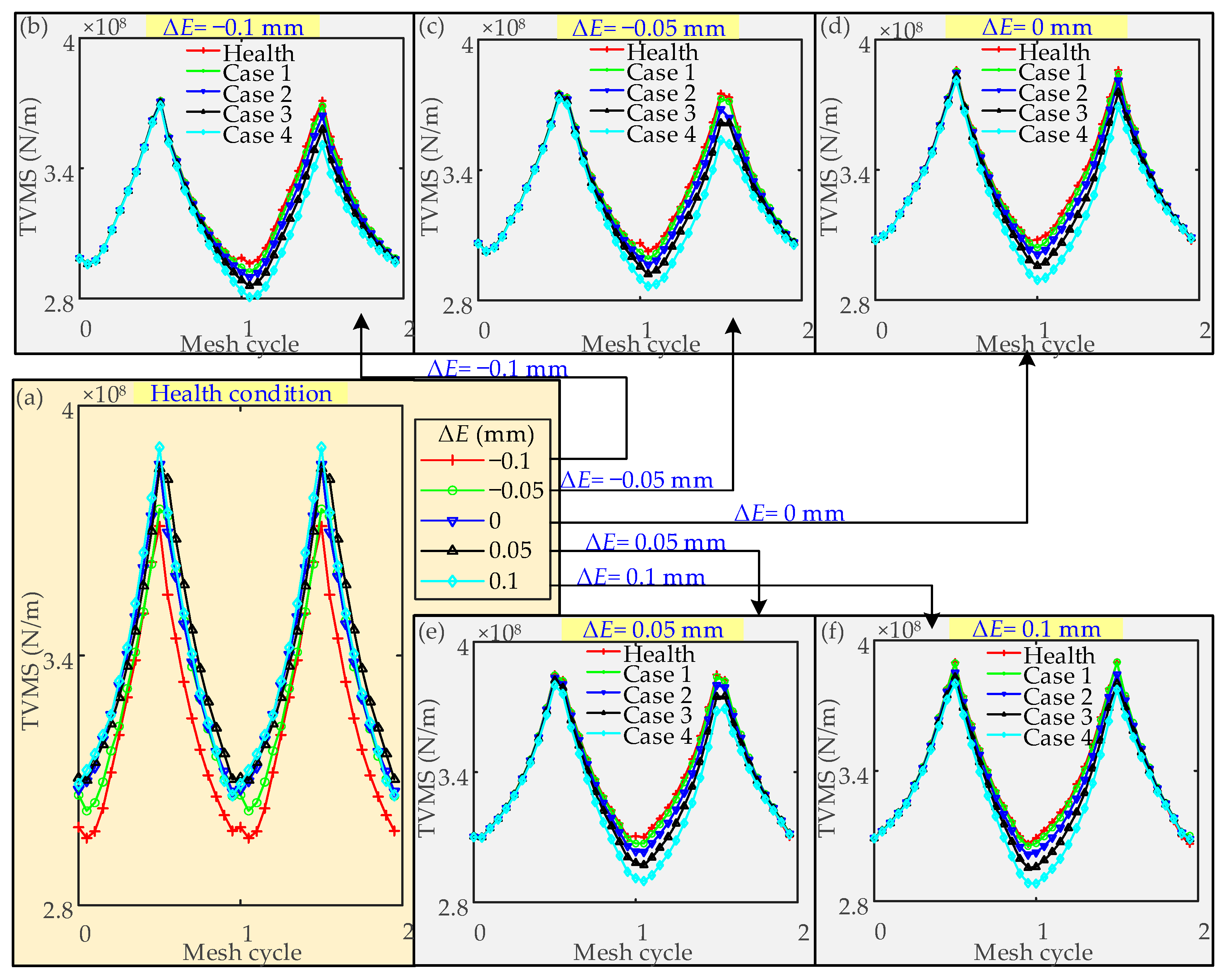
Figure 23.
Under the influence of offset error, the fluctuation of time-domain indicators relative to their respective healthy condition values under different degrees of cracks.
Figure 23.
Under the influence of offset error, the fluctuation of time-domain indicators relative to their respective healthy condition values under different degrees of cracks.

Figure 24.
Under the influence of offset error, the fluctuation of frequency-domain indicators relative to their respective healthy condition values under different degrees of cracks.
Figure 24.
Under the influence of offset error, the fluctuation of frequency-domain indicators relative to their respective healthy condition values under different degrees of cracks.

Table 1.
Blanks parameters.
| Parameter | Bevel Pinion | Bevel Gear |
|---|---|---|
| Tooth number z1/z2 | 17 | 81 |
| Modulus m (mm)/Shaft angle Σ (°)/Mean spiral angle β (°) | 5.6/90/35 | |
| Direction of rotation | Left-handed | Right-handed |
| Face width b (mm) | 60 | |
| Mean cone distance R (mm) | 201.741 | |
| Pitch angle δ (°) | 11.8530 | 78.1470 |
| Root angle δf (°) | 10.9321 | 76.1944 |
| Face angle δa (°) | 13.8056 | 79.0679 |
| Addendum height ha (mm) | 6.8480 | 2.6720 |
| Dedendum height hf (mm) | 3.7250 | 7.9010 |
Table 2.
Machine tool settings of bevel pinion.
| Parameter | Concave | Convex |
|---|---|---|
| Cutter point radius r01 (mm) | 226.47 | 230.86 |
| Pressure angle α01 (°) | −18.75 | 21.25 |
| Root fillet radius ρ01 (mm) | 1 | 1 |
| Machine center to back X1 (mm) | −5.237 | 8.545 |
| Sliding base XB1 (mm) | 15.217 | 13.183 |
| Blank offset E1 (mm) | 3 | 3.5 |
| Radial distance Sr1 (mm) | 197.762 | 209.634 |
| Machine root angle γm1 (°) | 7.7936 | 10.05 |
| Cradle angle q1 (°) | 71.6258 | 67.3267 |
| Tilt Angle i (°) | 2.7343 | 3 |
| Swivel angle j (°) | 286.2802 | 227.2839 |
| Velocity ratio i1 | 4.6799 | 5.2574 |
Table 3.
Machine tool settings of bevel gear.
| Parameter | Value |
|---|---|
| Cutter point radius r02 (mm) | 229.975(concave)/227.225(convex) |
| Pressure angle α02 (°) | −19(concave)/21(convex) |
| Root fillet radius ρ02 (mm) | 1.6 |
| Machine center to back X2 (mm) | 0 |
| Sliding base XB2 (mm) | 0 |
| Blank offset E2 (mm) | 0 |
| Radial distance Sr2 (mm) | 200.091 |
| Machine root angle γm2 (°) | 76.1944 |
| Cradle angle q2 (°) | 69.3682 |
| Velocity ratio i2 | 1.0212 |
Table 4.
Crack location and morphology parameters.
| Case 1 | Case 2 | Case 3 | Case 4 | |
|---|---|---|---|---|
| λ (mm) | 29.2 | 29.2 | 29.2 | 29.2 |
| δ (mm) | 4.43 | 8.46 | 12.48 | 16.51 |
| χ (mm) | 1.78 | 4.45 | 6.23 | 8.02 |
Table 5.
Time-domain statistical indicators.
| Name | Equation | Name | Equation |
|---|---|---|---|
| Average (A) | Crest (C) | ||
| Standard deviation (STD) | Impulse (I) | ||
| Square mean root (SMR) | Clearance (L) | ||
| Root mean square (RMS) | Peak-to-peak (PP) | ||
| Peak (P) | Skewness (S) | ||
| Waveform (W) | Kurtosis (K) |
Table 6.
Frequency-domain statistical indicators.
| Name | Equation | Name | Equation |
|---|---|---|---|
| F12 | F18 | ||
| F13 | F19 | ||
| F14 | F20 | ||
| F15 | F21 | ||
| F16 | F22 | ||
| F17 | F23 |
Table 7.
Crack location considering various offset errors.
| ΔE = −0.1 mm | ΔE = −0.05 mm | ΔE = 0 mm | ΔE = 0.05 mm | ΔE = 0.1 mm | |
|---|---|---|---|---|---|
| λ (mm) | 27.2 | 28.0 | 29.2 | 30.4 | 30.8 |
Table 8.
The max/min relative differences of TVMS under various crack degrees and offset errors.
| ΔE = −0.1 mm | ΔE = −0.05 mm | ΔE = 0 mm | ΔE = 0.05 mm | ΔE = 0.1 mm | |
|---|---|---|---|---|---|
| Relative Error Max/Min (%) | |||||
| Case 1 | 0.02/1.31 | 0.03/1.20 | 0.03/1.02 | 0.07/0.95 | 0.09/1.34 |
| Case 2 | 0.14/2.13 | 0.18/2.06 | 0.35/2.06 | 0.40/2.22 | 1.23/1.63 |
| Case 3 | 0.30/3.46 | 0.31/3.50 | 0.75/3.75 | 0.71/4.14 | 1.79/3.60 |
| Case 4 | 0.60/5.23 | 0.65/5.34 | 1.25/5.89 | 1.29/6.52 | 2.53/5.97 |
Publisher’s Note: MDPI stays neutral with regard to jurisdictional claims in published maps and institutional affiliations. |
© 2022 by the authors. Licensee MDPI, Basel, Switzerland. This article is an open access article distributed under the terms and conditions of the Creative Commons Attribution (CC BY) license (https://creativecommons.org/licenses/by/4.0/).
Share and Cite
MDPI and ACS Style
Han, H.; Ma, H.; Wang, H.; Zhu, J.; Li, Z.; Liu, Z. Dynamic Simulation of Cracked Spiral Bevel Gear Pair Considering Assembly Errors. Machines 2022, 10, 929. https://doi.org/10.3390/machines10100929
AMA Style
Han H, Ma H, Wang H, Zhu J, Li Z, Liu Z. Dynamic Simulation of Cracked Spiral Bevel Gear Pair Considering Assembly Errors. Machines. 2022; 10(10):929. https://doi.org/10.3390/machines10100929
Chicago/Turabian StyleHan, Hongzheng, Hui Ma, Haixu Wang, Jiazan Zhu, Zhanwei Li, and Zimeng Liu. 2022. "Dynamic Simulation of Cracked Spiral Bevel Gear Pair Considering Assembly Errors" Machines 10, no. 10: 929. https://doi.org/10.3390/machines10100929
Note that from the first issue of 2016, this journal uses article numbers instead of page numbers. See further details here.