
Research on Stiffness Identification Method for Complex Joints Based on Modal Correlation Analysis

School of Mechanical and Precision Instrument Engineering, Xi’an University of Technology, Xi’an 710048, China
*
Author to whom correspondence should be addressed.
Machines 2022, 10(11), 993; https://doi.org/10.3390/machines10110993
Submission received: 20 September 2022
/
Revised: 25 October 2022
/
Accepted: 27 October 2022
/
Published: 29 October 2022
(This article belongs to the Section Advanced Manufacturing)
Abstract
:The dynamic performance of mechanical systems is seriously affected by the stiffness of mechanical joints. The tool holder system of the deep hole machine tool was taken as the object; based on the modal correlation of experiment and finite element simulation, a simple and practical method was proposed to obtain the joint stiffness of the tool holder system under the structure form of the tool overhang of 200 mm. For the same tool holder system, the simulation and experimental analysis were carried out with different structural forms of tool overhang of 300 and 400 mm, which further verified the correctness and feasibility of the method for obtaining the joint stiffness, as well as provided a new idea and certain theoretical basis for extracting the joint stiffness of the tool holder system in deep hole machining.
1. Introduction
As an inherent structure of the mechanical system, the mechanical joint has complex dynamic characteristics with both elasticity and damping under the external load. It has a significant impact on the dynamic performance of the whole mechanical system. Studies have shown that the dynamic model error of the joint is the main factor in the dynamic model error of the entire mechanical system [1,2,3,4,5]. To obtain an accurate and reliable dynamic model of the mechanical system and improve the prediction accuracy of the dynamic response of the system model, accurate parameter identification and modeling of the joint have become a key issue and research hotspot in the area of vibration control and the performance evaluation of mechanical structures.
Methods for identifying the dynamic parameters of joints mainly include theoretical calculation methods, experimental methods and finite element simulation with experimental methods. The theoretical modeling of the contact parameters of the joint is mainly based on the Hertz contact theory or fractal geometry theory. Li and Etsion et al. [6] established a plastic deformation model between a rough surface and a rigid plane based on the Hertzian contact theory. Chang et al. [7] considered the elastic and plastic deformation of the asperity on the rough surface, combined with the principle of conservation of the asperity deformation volume and further proposed the model of Chang, Etsion, and Bogy (the CEB model). Kogut et al. [8] proposed the model of Kogut and Etsion (the K-E model) by using the finite element simulation results of a single asperity and statistical theory to extend the research to the contact behavior between two rough surfaces. Majumdar and Bhushan [9] proposed the model of Majumdar and Bhushan (the MB contact fractal model) and established the expression of the normal load of the rough surface asperity based on the theory of fractal characteristics.
However, due to the randomness and uncertainty of the contact of the asperities, it is difficult to reveal the true contact mechanism of the joints accurately. In addition, it is impossible to directly apply these theoretical analytical models to complex mechanical joint calculation and modeling.
Compared to the numerical analysis method, experimental data are reflections of the physical structure, which is the standard for evaluating the reliability of a model [10]. Therefore, with the aid of experimental modal data, finite element modeling and inverse identification of parameters for complex joints can be carried out without the influence of various ideal assumptions in the analytical model. It is also not necessary to consider factors such as multiple connection methods, lubricating media, surface morphology, the heat treatment state of the joint, as well as the problem of the narrow application scope of the existing analysis method [11,12,13]. There are two main types of finite element models for the joint. The first is the finite element model of the joint based on spring damping elements. Ahmadian et al. [14] used the nonlinear spring damping elements to model and identify the damping of bolt joints. Hu et al. [15] also used nonlinear spring elements to model the bolted T-stub connections and analyzed the mechanical characteristics of the specimen under cyclic loading. Kim et al. [16] also equated the joint as a spring element, establishing a numerical model of the joint under different joint conditions and verifying the correctness of the numerical model through modal experiments. The second type is the finite element model of the joint based on equivalent virtual materials. Iranzad [17] established a virtual material model of the nonlinear characteristics of the bolt joint and obtained the physical characteristics of the virtual material in the model through testing. Ahmadian et al. [18,19,20] treated the mechanical joint as a thin layer of virtual material and identified the elastic modulus and Poisson’s ratio of the thin layer material through modal experiments. Hui et al. [21] established the finite element equivalent model of the bolt joint based on the virtual material layer method and calculated the elastic modulus and Poisson’s ratio of the virtual material. Guo et al. [22] applied the idea of virtual material to modeling of the spindle-handle joint and established the dynamic balance equation of virtual material parameters. The above methods for identification of joint parameters mainly focus on the typical and simple contact surfaces. Once the joint is more complex, or there are multiple contact surfaces coupling, the modeling of the simulation model becomes more troublesome and more uncertain, so there is a need for a simpler and more practical method to identify the joint parameters.
Based on the modal correlation between the experiment and the finite element simulation, this paper takes the tool holder system of the deep hole machine tool as the research object and proposes a method to obtain the stiffness of complex joints using the principle that the position and size of the tool holder system determine the modal characteristics of the tool. In the structure form of a tool overhang of 200 mm, the complex experimental object, composed of the tool holder and a tool, is transformed into a regular and simple tool by taking the whole tool holder system as a constraint condition and the modal experiment of the tool is completed. The tool holder system’s multiple joints are set up as spring units, the finite element model of the tool containing the joint information was established and the modal analysis was carried out. The frequency correlation between the experimental and simulated modes of the tool is solved and the regression analysis is carried out. The vibration pattern correlation analysis is also performed for the two modes to complete the identification of the stiffness of the tool holder. Based on the results of the stiffness identification, the modal experiment and finite element simulation were carried out for the structure forms with the tool overhang of 300 and 400 mm. The error analysis proves the correctness and feasibility of the proposed method.
2. Materials and Methods
2.1. Model Profile
The Boring and Trepanning Association (BTA) deep hole machine tool is a piece of special equipment for the deep hole machining of hard and brittle materials, as shown in Figure 1.
Since the processing quality of hard and brittle material is quite sensitive to the stability of the processing system, the tool holder system used to support the tool is the core component to ensure the stability of the processing system. The tool holder system of this equipment is composed of fixed support, radial bearing, wear-resistant axle sleeve, sealing ring, etc. Among them, the fixed support is fixed on the workbench to bear the radial load generated by the radial bearing in the processing process. As shown in Figure 2, the wear-resistant axle sleeve and the drilling tool for transition coordination bear the radial load of the tool and play the role of sliding bearing. According to the figure, the dynamic characteristics of the tool holder system are not only affected by the fixed support, radial bearing, and wear-resistant axle sleeve but by the dynamic characteristics of three contact surfaces formed between the fixed support and radial bearing, the radial bearing and wear-resisting axle sleeve, as well as the wear-resisting axle sleeve and drilling tool, which is the main error source of the dynamic model. Therefore, the identification of the joint’s parameters is essential for the dynamic modeling of the machining system.
According to the machining principle of the BTA deep hole machine tool and the force situation of the tool during the machining, the single tool holder system can be treated as a whole radial spring unit and the equivalent model of its machining system is shown in Figure 3. The tool overhang length is defined as the distance between the right hand tool holder and the tool end face.
According to Figure 3, the dynamic model of the machining system can be simplified to a free vibration model of a multi-span continuous beam composed of the two radial spring units and a drilling tool. The position and size of the two radial spring units determine the modal characteristics of the drilling tool. Using this principle, the frequency correlation between the experimental and simulated modes of the drilling tool, is used as the solution target. The design of experiment (DOE) of the stiffness value of the two spring units is designed and regression analyzed. Correlation analysis of the vibration patterns of the two modes is performed to complete the inverse identification of parameters of the two radial spring units. Finally, modal experiments and simulations, with different tool overhang lengths, are performed to verify the reliability of the stiffness values determined by the correlation analysis. The flowchart is shown in Figure 4.
2.2. Modal Correlation Theory
Theoretically, the modal test analysis is an actual analysis of a structure, and the results obtained are more reliable. On the other hand, the finite element modal analysis is a theoretical calculation completed after making a lot of assumptions and simplifications to the structural model, and the results are often different from the actual situation and less credible. Therefore, in order to verify the consistency between the finite element modal and the experimental modal, correlation analysis is usually carried out on the results of the two modes.
Modal correlation analysis is an analysis method used to judge the degree of conformity between the experimental model and the finite element model. The analysis methods mainly include frequency correlation analysis and mode shape correlation analysis [23,24,25].
- Frequency correlation: The natural frequency is the basic attribute of the modal parameters of the structure, and it is easier to measure accurately than the modal shape, so the frequency correlation is more widely used. The correlation is usually expressed as:where: is the coefficient of correlation, is the calculated mode frequency, is the experimental mode frequency.
- Vibration mode correlation: While the modal shape is a description of structural vibration displacement in space, modal frequency is a description of structural vibration characteristics in time. Only by combining them can a complete description of structural vibration be achieved and the accuracy of the model correction be improved. The modal assurance criterion (MAC) value between the experimental and finite element modal vectors can be obtained by the following equation:where: is the modal vector of a EMA modal shape; is the transpose of ; is the modal vector of a FEA modal shape; is the transpose of .
3. Results
3.1. Experimental Modal Analysis (EMA)
The natural frequency, vibration type and frequency response function of the mechanical structure are the main parameters to describe its dynamic characteristics. Modal experiment on the structure is the most direct and effective way to obtain the above parameters. The diameter of the tool used in this experiment is Φ130 mm, with a wall thickness of 2 mm and a length of 815 mm. The tool holder system is installed on the workbench. The spindle of the machine tool is then disconnected to obtain the structure state of the tool overhang with 200 mm. The modal experiment was carried out on the trepanning drill tool. To improve the accuracy of the modal experiment, the single input/multiple output (SIMO) modal parameter identification method is used in this experiment and the experimental data are collected and analyzed by LMS test.lab software (SIEMENS AG, Berlin, Germany).
To obtain the natural frequencies and effective vibration types of modal experiments accurately, the arrangement of excitation points and vibration pick-up points should be reasonable. According to the results of pre-experiment and finite element simulation, the first few order natural frequency and vibration type of the tool all appear in the radial direction, so the excitation points and vibration pick-up points of the test are arranged in the radial direction of the tool. To measure the excitation of the tool as accurately as possible, the arrangement of excitation points is as follows: the tool is divided into 8 sections in the axial direction and each end face (including the front and end faces) is arranged with 8 excitation points, a total of 72. The arrangement of vibration pick-up points is as follows: 6 vibration pickup points are evenly arranged on different end faces and angles in the radial direction of the tool. The sensor layout points and the experimental site are shown in Figure 5.
To minimize the influence of random experimental errors and improve the reliability of experimental data, each excitation point is vertically excited three times along the radial direction. The composition of the modal experimental device is shown in Table 1.
The collected data signals were analyzed and processed with LMS Test.Lab software. The frequency range was selected from 0 to 1600 Hz. The natural frequencies of the first seven-order experiments, obtained by the peak picking method, and the corresponding vibration types of each order are shown in Table 2. The natural frequency and vibration type, obtained from the modal experiment, were used as the reference values for the correlation analysis with the natural frequency and vibration type obtained from the simulation calculation of the finite element model.
MAC is a mathematical criterion to check the correlation of two modal vibration vectors and is used to evaluate the quality of identification of the experimental modal parameters and to verify the reliability of the experimental data. Its MAC value is defined as [25]:
where: and are the values of the degrees of freedom corresponding to the n sensors in the calculated mode shapes of the i order and the j order, respectively.
According to definition of the MAC value, the two vectors representing the same order mode are linearly correlated and their MAC value should be close to 1 (100 when the percentage represents MAC value). The two vectors representing different order modes are linearly independent and their MAC values should be close to 0. The 3D bar chart of MAC between the modal vibration vectors obtained in this experiment is shown in Figure 6, which shows that the MAC value between the two vectors of the same physical mode is 100%, and the MAC value between the two vectors of different modes is less than 20%, which complies with the modal confidence criterion. Based on the modal MAC matrix and the vibration types of each mode, the results of the modal experiment are reliable.
3.2. Frequency Correlation Analysis
In this paper, LMS Virtual.Lab is used to carry out the finite element modeling and modal correlation analysis of the tool and the holder system. A reasonable and accurate finite element model is the basis for the dynamic characteristic analysis. According to the characteristics of finite element theory calculation, in order to improve the accuracy and efficiency of finite element calculation and analysis, it is necessary to simplify the geometric model of the tool as follows: by ignoring the small steps and teeth of the tool head as well as the small holes at the end of the tool and the handle that can cause local modes. Since the drill tool only bears the radial load of the fixed support, the joint only has the radial stiffness. According to the actual assembly situation, a radial spring damping unit is established between the drill tool and the fixed support. Because the interference fit is between the fixed support, radial bearing, and wear-resisting sleeve, the damping of the joint is very small. Therefore, the small effect of damping on the natural frequency is ignored.
The model focuses on the overall stiffness of the tool holder system, so it is necessary to simplify the complex modeling process between the joints of the tool holder system and model it as an integral spring unit. The model adopts the user-defined elastic spring elements provided by LMS Virtual.Lab to establish the dynamic finite element model containing the joint information, as shown in Figure 7.
According to the pre-experiment of the simulation model and the related theory of the joint, the DOE value range of the stiffness of the two spring elements is determined to be 1 × 10⁷–3 × 10⁷ N/m. Latin hypercube sampling (LHS) was used to DOE design the stiffness values of the two spring elements. As a stratified sampling method, LHS has become an important method to fill the design space because of its good distribution uniformity, representation of the whole solution space, and random search function.
According to the random rules of LHS sampling, 30 times of independent sampling are carried out for the two spring elements in the designed sampling space. Then, the corresponding simulation calculations are performed for each scenario separately using the established finite element simulation model; the simulation results are statistically analyzed and the frequency correlation coefficient γ is calculated. The seven orders frequency correlation coefficients, γ1, γ2, γ3…γ7, calculated for different spring units stiffness K1 and K2, are shown in Table 3.
There is a correlation and a significant corresponding trend between spring unit stiffness K1, K2, and frequency correlation coefficient γ, which is the basis for regression analysis of the frequency correlation coefficient γ. Therefore, it is necessary to analyze the correlation between the two groups of variables. According to the theory of correlation analysis, the correlation and significance of the two groups of variables are tested and the results are shown in Table 4.
The results of correlation analysis show that the spring element stiffness K1 and K2 have a significant effect on the frequency correlation coefficients γ1 and γ5 but have no effect on the frequency correlation coefficients γ2, γ3, γ4, γ6, and γ7. Therefore, the frequency correlation of the first and the fifth order was studied as the target of regression analysis. To improve the fitting accuracy of the frequency correlation function, the corresponding relationship between different spring element stiffness and frequency correlation coefficient γ1, γ5 was further analyzed intuitively. According to the definition of frequency correlation, studying the trend between the simulated modal frequency and the spring unit stiffness alone cannot fully explain the relationship between them, but the modal frequency error between the simulation and experiment can well reflect the relationship between them. The variation trend of the first and fifth order frequency difference, with different spring element stiffness, is shown in Figure 8.
In Figure 8, the frequency difference of the first- and fifth-order modes increases with the increase in the stiffness of the spring unit and both of them have a linear trend.
The polynomial surface function is used to regression fit the first- and fifth-order frequency correlation coefficients. The higher order of the K term of the polynomial surface function is 1 due to a linear trend between the frequency difference and the spring unit stiffness. The regression models for the first frequency correlation coefficient γ1 and the fifth frequency correlation coefficient γ5 are shown in Equations (4) and (5), respectively.
From the established regression models, the response surfaces of γ1 and γ5, under different spring element stiffness, can be obtained, as shown in Figure 9. From the figure, both γ1 and γ5 increase with the stiffness of the two spring units and γ1 is more sensitive to changes in the stiffness values of the two spring units. At the position of the comprehensive minimum value of γ1 and γ5, K1 and K2 are taken as the optimal solution for the equivalent dynamic stiffness of the joint, as shown in Figure 10. K1 and K2 are 1.12 × 10⁷ N/m and 1.72 × 10⁷ N/m, respectively. These values are the result of the joint parameter identification.
3.3. Modal Shape Correlation Analysis
For the modal correlation, the mode shape correlation needs to be considered when analyzing the frequency correlation, especially for complex structures or structures with dense modes. In practice, it is necessary to conduct a correlation analysis of the frequency and mode shape of the model at the same time to determine the corresponding relationship between the simulation model and the experimental model and further judge the accuracy of the finite element model.
Since the experimental vibration mode is a wireframe model described by the vibration displacement data of 72 measurement points, the finite element simulation model is described by thousands of finite element grids. Therefore, it is necessary to transform the finite element model into a wireframe model similar to the modal experiment and evaluate the degree of conformity between the two wireframe models. The fitting degree of the experimental wireframe model and the simulation wireframe model is shown in Figure 11. The fitting errors of both are minimal and the measurement points of the mode experiment can well reflect the displacement change of the corresponding position of the finite element model.
According to the results of frequency correlation analysis, the difference between the two models can be analyzed qualitatively or quantitatively. If the difference between the two models is below the user-defined threshold, the theoretical model is considered to be precise and without correction. Otherwise, the theoretical model needs to be corrected through the finite element model modification technique. The first seven-order modal shapes of the experiment and simulation are compared qualitatively, and the results are shown in Table 5. The modal shapes of the two have a good consistency. The first- and fifth-order vibration types are the overall deformation of the trepanning drill tool, and the rest are the local deformation of the trepanning drill tool.
According to the mode shape correlation theory, the first seven modes of experiment and simulation are quantitatively analyzed. They were analyzed using the Modal Correlation module in LMS Virtual.Lab software, and the MAC values of the Modal shape vectors from the experiment and finite element simulation were analyzed. The calculated values are shown in Figure 12.
The MAC values of the modes between the same order are all greater than 0.6, and the MAC values of the modes between the different orders are all less than 0.1, which meets the requirements of the modal shape correlation. It is proved that the experimental mode and the simulated mode have good consistency, and the accuracy of the finite element equivalent model has also been further verified.
4. Discussion
To further verify the correctness and validity of obtaining the stiffness of the tool holder system, different tool overhangs were selected to analyze the tool’s natural frequency errors. The identified equivalent stiffness information of the tool holder system is substituted into the finite element simulation model with the tool overhangs of 200 mm, 300 mm, and 400 mm, and the natural frequencies of the tools under different structural forms were calculated, while the tool modal experiments under different structural forms were completed to verify the universality of the identified stiffness. The experimental and simulation values of the natural frequencies of the tool under the three structural forms are shown in Figure 13 and the natural frequencies of the three structural forms have a good consistency.
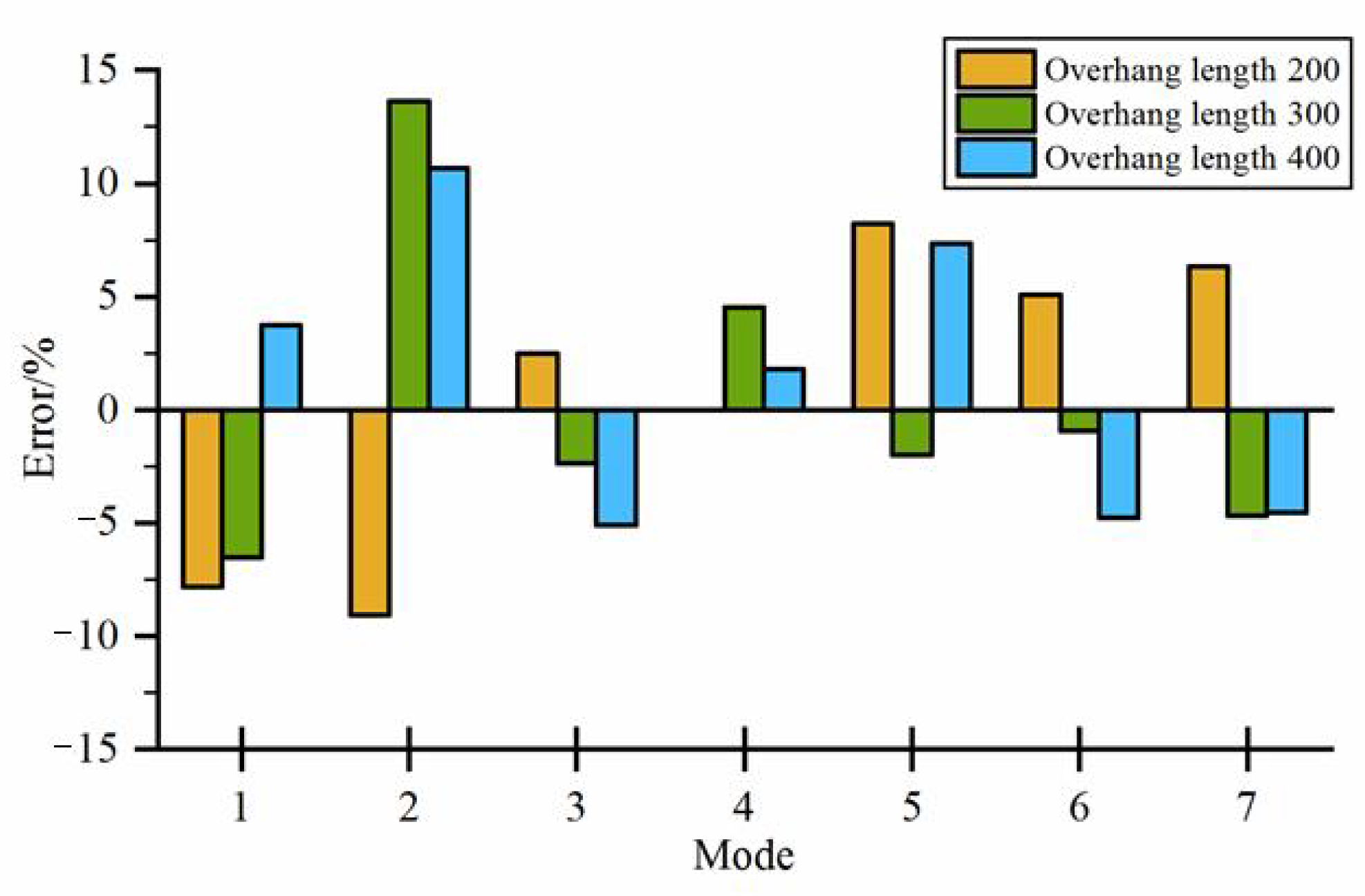
By calculating the natural frequencies in Figure 13, the natural frequency errors of each order mode under different structural forms are obtained, as shown in Figure 14. The error between the simulated and experimental values of the natural frequency of each order mode is less than 10%, except for the second-order mode. The error of different structural forms has both positive and negative errors, which fully meet the requirements of engineering applications. It proves the correctness and reliability of the stiffness identification results. It also confirms the method’s feasibility in obtaining the stiffness of complex joints based on the modal correlation. Table 5 shows the second-order mode is the local deformation of the drilling tool head part. The significant second-order mode frequency error of the three structural forms may be that the head of the tool is composed of 12 teeth and gaps. The finite element modeling simplifies these gaps, resulting in the significant local mode error of the finite element model.
5. Conclusions
In the modal experiment process, only the tool is modeled and analyzed and the tool holder system and its supporting elements are unified as constraints, turning the complex tool holder system and tool experiment objects into regular and simple tools, which significantly simplifies the modeling and implementation difficulties of the modal experiment. In the finite element modeling process, multiple complex combinations of the tool holder system are treated as integral spring units, which simplifies the complex modeling process between the joints. The following conclusions can be obtained.
- (1)
- Compared with the current research on the identification of joint parameters, which focuses on the equivalent distribution of spring units or the parameter setting of virtual material physical properties for a typical, single joint, this paper focuses on the three contact surfaces formed by four components and their influence on the structural system as a whole, simplifying the connection relationship between the three joints and the specific situation of individual joints. At the same time, in the selection of experimental objects, all components forming the joint, are not taken as the experimental objects, but the components significantly affected by the parameters of the joint are taken as the experimental objects. The method is quite convenient to use in engineering. It can effectively avoid the errors caused by too many harsh assumptions in analytical modeling, especially since the advantages of parameter identification for complex and multiple joints are more pronounced and the errors meet the requirements of engineering use.
- (2)
- When the position of the radial spring unit is determined, the magnitude of its stiffness affects the overall mode of the trepanning drill tool, while the local mode of the tool is only affected by the position of the radial spring unit, independent of its size.
- (3)
- The error analysis results show that, except for the second mode, the natural frequency errors of other modes are less than 10%. In Figure 2, it can be seen that there are many gaps on the tool head and the thickness of the teeth is slightly thicker than the tool body, which is extremely unfavorable to the finite element modeling and it is impossible to realize the modal experiment on this part. Therefore, this part is simplified in the finite element modeling and modal experiments. This simplification only changes the structural form of the tool head and does not change the overall structural form of the tool. It does not affect the accuracy of the model on other parts of the tool. In Table 5, the structural deformation of the second-order mode occurs precisely in the tool head. Therefore, the larger error in the second-order natural frequency is a normal situation due to the local simplification of the tool head in both finite element modeling and the modal experiments.
Author Contributions
Conceptualization, R.Y. and S.L.; methodology, R.Y. and L.L.; software, R.Y.; validation, R.Y.; formal analysis, R.Y. and S.L.; investigation, R.Y.; resources, R.Y. and S.L.; data curation, R.Y. and L.L.; writing—original draft preparation, R.Y.; writing—review and editing, F.L. and K.W. All authors have read and agreed to the published version of the manuscript.
Funding
The research is financially supported by the National Natural Science Foundation of China (No. 51575442) and the Natural Science Foundation of Shaanxi Province (No. 2016JZ011).
Institutional Review Board Statement
Not applicable.
Informed Consent Statement
Not applicable.
Data Availability Statement
Not applicable.
Acknowledgments
The authors are grateful to National Natural Science Foundation of China and Natural Science Foundation of Shaanxi Province, which enabled the research to be carried out successfully.
Conflicts of Interest
The authors declare no conflict of interest.
References
- Ibrahim, R.A.; Pettit, C.L. Uncertainties and dynamic problems of bolted joints and other fasteners. J. Sound Vib. 2005, 279, 857–936. [Google Scholar] [CrossRef]
- Zaman, I.; Khalid, A.; Manshoor, B.; Araby, S.; Ghazali, M.I. The effects of bolted joints on dynamic response of structures. IOP Conf. Ser. Mater. Sci. Eng. 2013, 50, 012018. [Google Scholar] [CrossRef] [Green Version]
- Adel, F.; Shokrollahi, S.; Jamal-Omidi, M.; Ahmadian, H. A model updating method for hybrid composite/aluminum bolted joints using modal test data. J. Sound Vib. 2017, 396, 172–185. [Google Scholar] [CrossRef]
- Shamine, D.M.; Hong, S.W.; Shin, Y.C. Experimental Identification of Dynamic Parameters of Rolling Element Bearings in Machine Tools. J. Dyn. Syst. Meas. Control 2000, 122, 95–101. [Google Scholar] [CrossRef]
- Zhang, G.P.; Huang, Y.M.; Shi, W.H.; Fu, W.P. Predicting dynamic behaviours of a whole machine tool structure based on computer-aided engineering. Int. J. Mach. Tools Manuf. 2003, 43, 699–706. [Google Scholar] [CrossRef]
- Li, L.; Etsion, I.; Ovcharenko, A.; Talke, F.E. The Onset of Plastic Yielding in a Spherical Shell Compressed by a Rigid Flat. J. Appl. Mech. 2011, 78, 011016. [Google Scholar] [CrossRef]
- Chang, W.R.; Etsion, I.; Bogy, D.B. An Elastic-Plastic Model for the Contact of Rough Surfaces. J. Tribol. Int. 1987, 109, 257–263. [Google Scholar] [CrossRef]
- Kogut, L.; Etsion, I. A Finite Element Based Elastic-Plastic Model for the Contact of Rough Surfaces. Tribol. Trans. 2003, 46, 383–390. [Google Scholar] [CrossRef]
- Majumdar, A.; Bhushan, B. Fractal Model of Elastic-Plastic Contact Between Rough Surfaces. J. Tribol. 1991, 113, 1–11. [Google Scholar] [CrossRef]
- Nobari, A.S.; Robb, D.A.; Ewins, D.J. A new approach to modal-based structural dynamic model updating and joint identification. Mech. Syst. Signal Process. 1995, 9, 85–100. [Google Scholar] [CrossRef]
- Mehrpouya, M.; Sanati, M.; Park, S.S. Identification of joint dynamics in 3D structures through the inverse receptance coupling method. Int. J. Mech. Sci. 2016, 105, 135–145. [Google Scholar] [CrossRef]
- Fritzen, C.-P. Identification of Mass, Damping, and Stiffness Matrices of Mechanical Systems. J. Vib. Acoust. Stress Reliab. Des. 1986, 108, 9–16. [Google Scholar] [CrossRef]
- Wang, M.; Wang, D.; Zheng, G. Joint dynamic properties identification with partially measured frequency response function. Mech. Syst. Signal Process. 2012, 27, 499–512. [Google Scholar] [CrossRef]
- Ahmadian, H.; Jalali, H. Identification of bolted lap joints parameters in assembled structures. Mech. Syst. Signal Process. 2007, 21, 1041–1050. [Google Scholar] [CrossRef]
- Hu, J.W.; Leon, R.T.; Park, T. Mechanical modeling of bolted T-stub connections under cyclic loads Part I: Stiffness modeling. J. Constr. Steel Res. 2011, 67, 1710–1718. [Google Scholar] [CrossRef]
- Kim, S.-M.; Ha, J.-H.; Jeong, S.-H.; Lee, S.-K. Effect of joint conditions on the dynamic behavior of a grinding wheel spindle. Int. J. Mach. Tools Manuf. 2001, 41, 1749–1761. [Google Scholar] [CrossRef]
- Iranzad, M.; Ahmadian, H. Identification of nonlinear bolted lap joint models. Comput. Struct. 2012, 96–97, 1–8. [Google Scholar] [CrossRef]
- Ahmadian, H.; Mottershead, J.E.; James, S.; Friswell, M.I.; Reece, C.A. Modelling and updating of large surface-to-surface joints in the AWE-MACE structure. Mech. Syst. Signal Process. 2006, 20, 868–880. [Google Scholar] [CrossRef]
- Ahmadian, H.; Jalali, H.; Mottershead, J.; Friswell, M. Dynamic modeling of spot welds using thin layer interface theory. In Proceedings of the Tenth International Congress on Sound and Vibration, Stockholm, Sweden, 7–10 July 2003; pp. 7–10. [Google Scholar]
- Ahmadian, H.; Ebrahimi, M.; Mottershead, J.E.; Friswell, M.I. Identification of bolted-joint interface models. Proc. ISMA 2002, 4, 1741–1747. [Google Scholar]
- Ye, H.; Huang, Y.; Li, P.; Li, Y.; Bai, L. Virtual material parameter acquisition based on the basic characteristics of the bolt joint interfaces. Tribol. Int. 2016, 95, 109–117. [Google Scholar] [CrossRef]
- Guo, H.; Zhang, J.; Feng, P.; Wu, Z.; Yu, D. A virtual material-based static modeling and parameter identification method for a BT40 spindle–holder taper joint. Int. J. Adv. Manuf. Technol. 2015, 81, 307–314. [Google Scholar] [CrossRef]
- Ouisse, M.; Foltête, E. Model correlation and identification of experimental reduced models in vibroacoustical modal analysis. J. Sound Vib. 2015, 342, 200–217. [Google Scholar] [CrossRef] [Green Version]
- Magalhães, F.; Caetano, E.; Cunha, Á. Operational modal analysis and finite element model correlation of the Braga Stadium suspended roof. Eng. Struct. 2008, 30, 1688–1698. [Google Scholar] [CrossRef]
- Allemang, R.J. The Modal Assurance Criterion (MAC): Twenty Years of Use and Abuse. Sound Vib. 2003, 37, 14–23. [Google Scholar]
Figure 1.
BTA deep-hole trepanning machine tool.
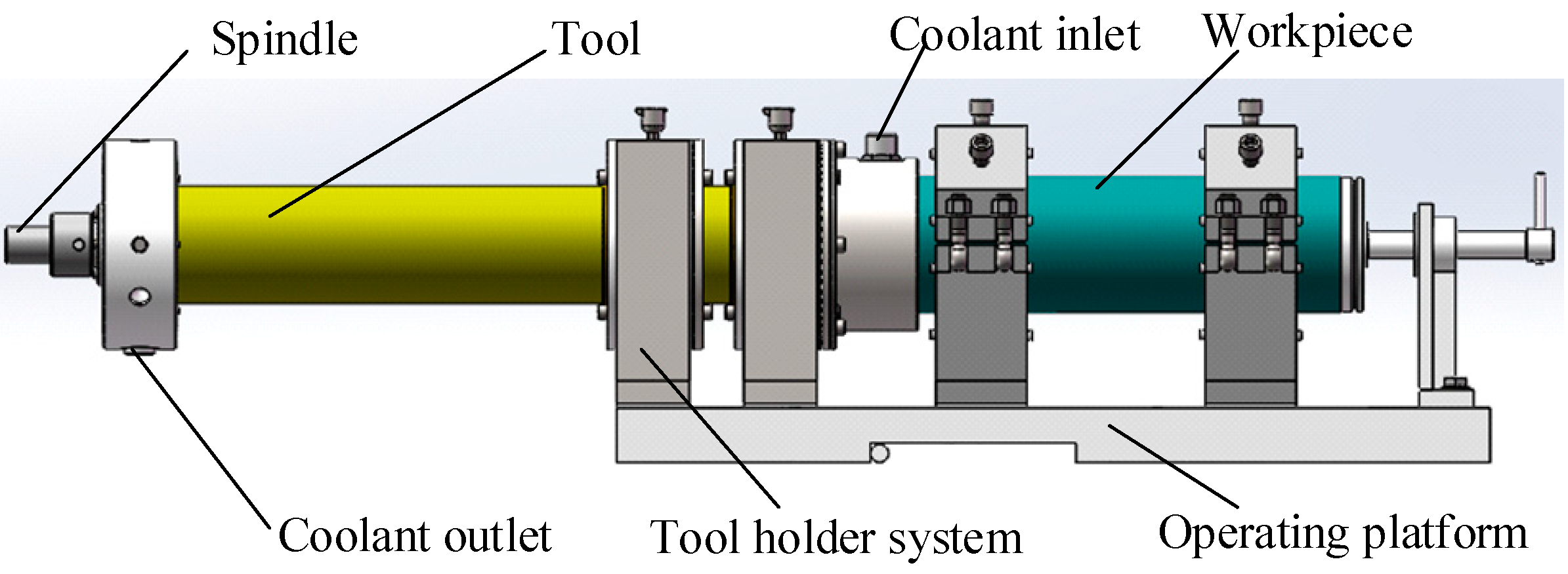
Figure 2.
Tool holder system.
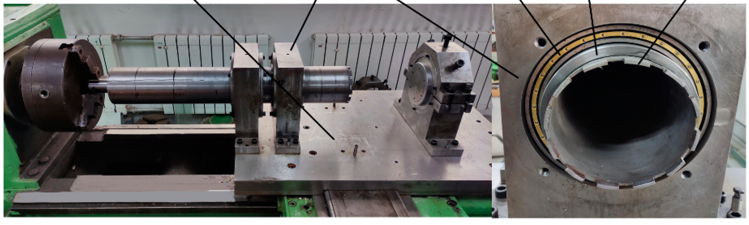
Figure 3.
Equivalent model of the machining system.
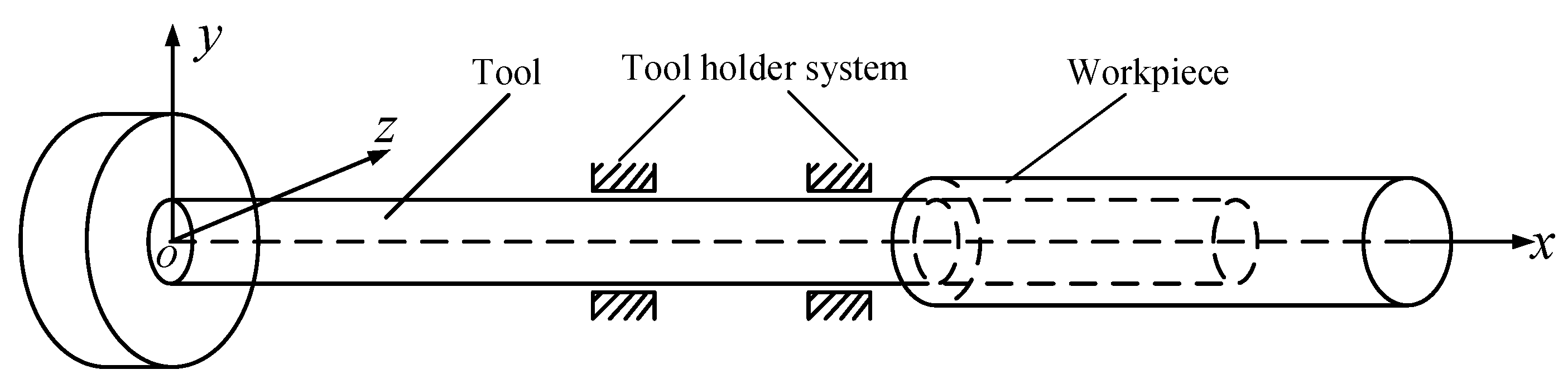
Figure 4.
Flowchart of inverse identification for the parameters of joints.

Figure 5.
Sensor layout position and experimental site.
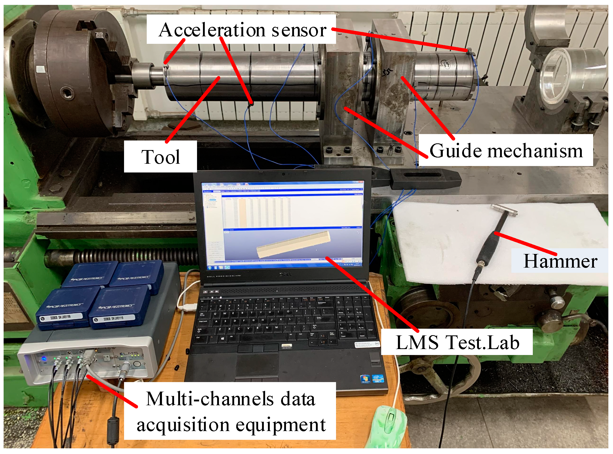
Figure 6.
MAC of experimental mode.
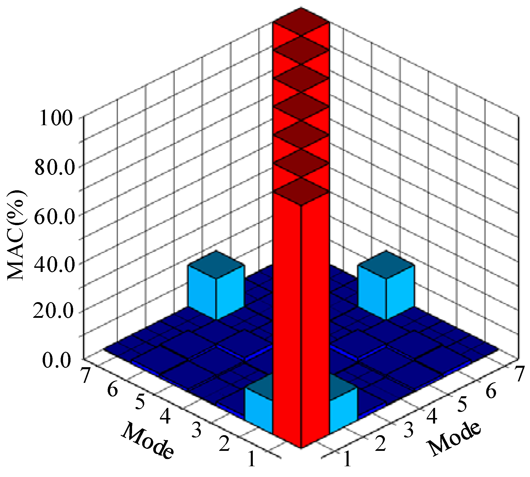
Figure 7.
The finite element model.
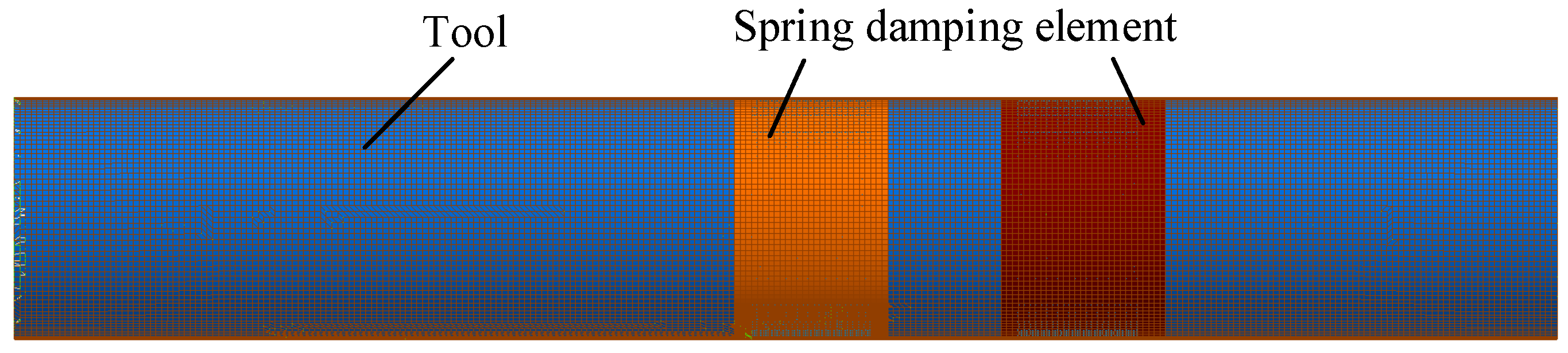
Figure 8.
Variation trend of frequency difference with different spring stiffness. (a) The first mode. (b) The fifth mode.
Figure 8.
Variation trend of frequency difference with different spring stiffness. (a) The first mode. (b) The fifth mode.

Figure 9.
Response surface of γ1 and γ5 under different spring element stiffness. (a) The first mode. (b) The fifth mode.
Figure 9.
Response surface of γ1 and γ5 under different spring element stiffness. (a) The first mode. (b) The fifth mode.
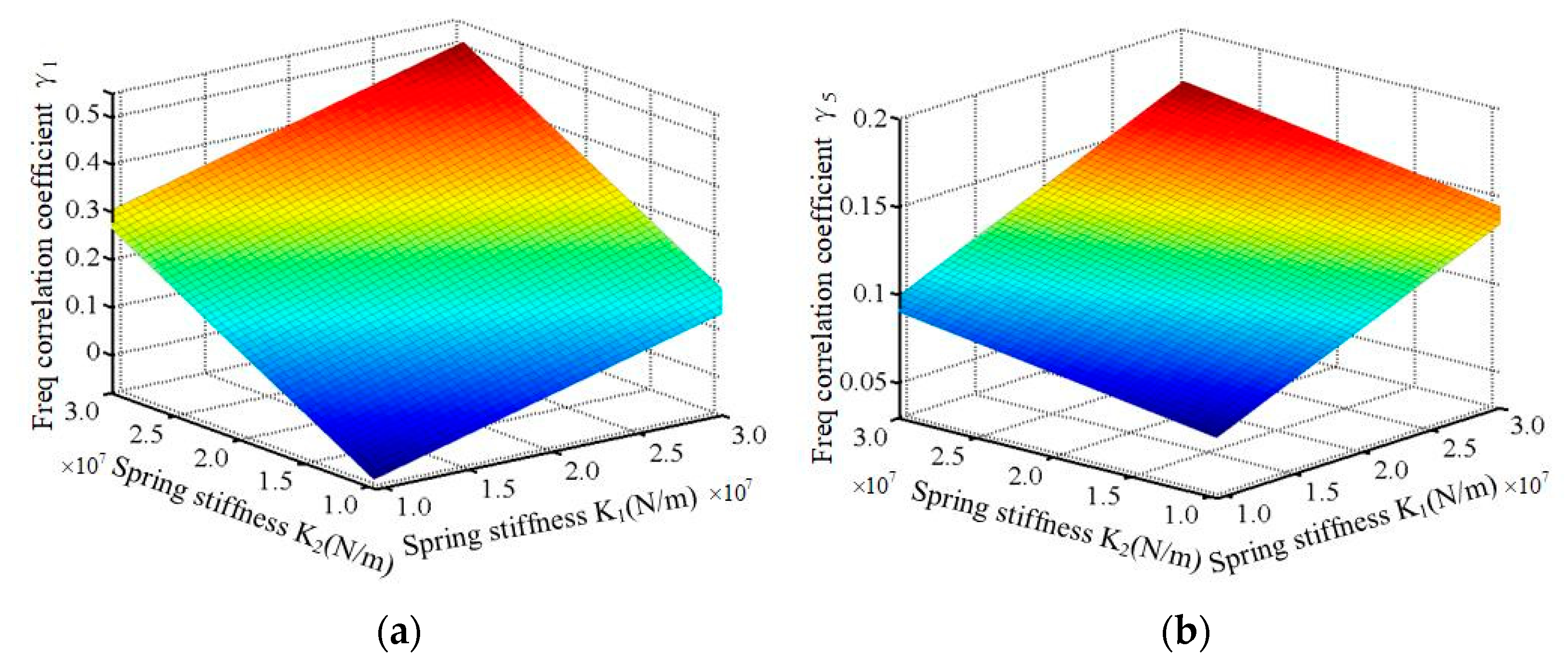
Figure 10.
Composite curve of γ1 and γ5.

Figure 11.
Wireframe models for EMA vs. FMA.
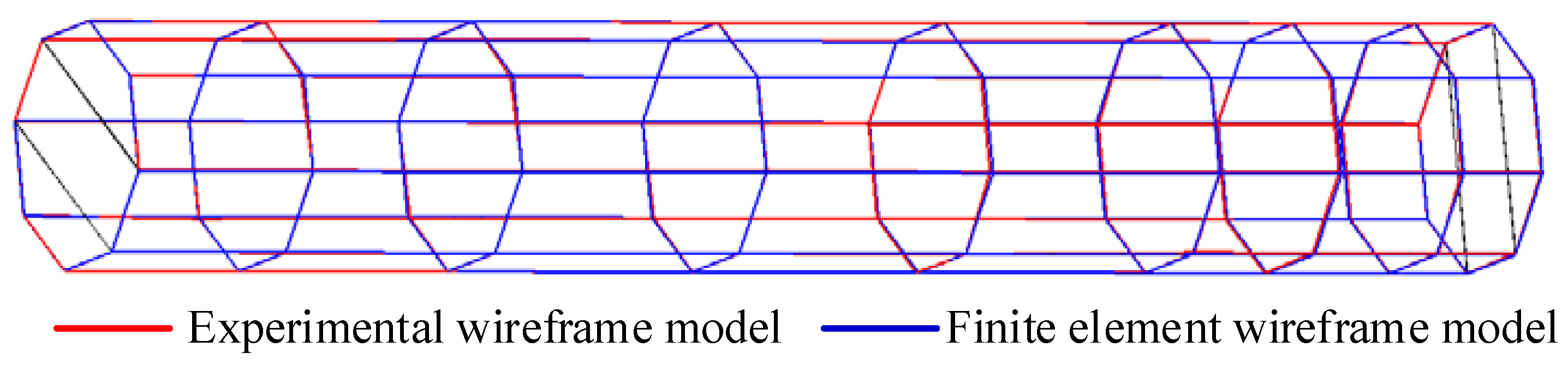
Figure 12.
MAC for EMA vs. FMA vibration modes.

Figure 13.
Natural frequency value under three working conditions. (a) The tool overhang length is 200 mm. (b) The tool overhang length is 300 mm. (c) The tool overhang length is 400 mm.
Figure 13.
Natural frequency value under three working conditions. (a) The tool overhang length is 200 mm. (b) The tool overhang length is 300 mm. (c) The tool overhang length is 400 mm.

Figure 14.
Natural frequency error under three working conditions.

Table 1.
Modal experimental equipment.
| Device | Model | Intent |
|---|---|---|
| Force hammer | PCB 086C03 | Generates the shock force signal |
| Acceleration sensor | PCB 333B30 | Obtains the force response signal |
| Multichannel data collector | LMS SCM09 | Collects data |
| Test analysis software | LMS Test.Lab | Data analysis and identification of modal parameters |
Table 2.
The experimental natural frequency values and vibration types.
| Order | Frequency (Hz) | Vibration type |
|---|---|---|
| 1 | 380.3 |  |
| 2 | 462.5 |  |
| 3 | 788.5 | 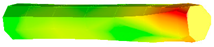 |
| 4 | 926.4 |  |
| 5 | 1039.5 |  |
| 6 | 1430.0 |  |
| 7 | 1526.5 |  |
Table 3.
Seven orders frequency correlation coefficients.
| Serial Number | K1/107 (N/m) | K2/107 (N/m) | γ1 | γ2 | γ3 | γ4 | γ5 | γ6 | γ7 |
|---|---|---|---|---|---|---|---|---|---|
| 1 | 2.03 | 2.26 | 0.268 | 0.091 | 0.026 | 0.001 | 0.120 | 0.038 | 0.064 |
| 2 | 2.30 | 1.30 | 0.140 | 0.091 | 0.026 | 0.001 | 0.117 | 0.038 | 0.064 |
| 3 | 2.50 | 1.03 | 0.113 | 0.091 | 0.026 | 0.001 | 0.120 | 0.038 | 0.064 |
| 4 | 2.15 | 2.72 | 0.342 | 0.091 | 0.026 | 0.001 | 0.130 | 0.038 | 0.064 |
| 5 | 1.70 | 2.63 | 0.296 | 0.091 | 0.026 | 0.001 | 0.113 | 0.038 | 0.064 |
| 6 | 2.62 | 1.87 | 0.259 | 0.091 | 0.026 | 0.001 | 0.135 | 0.038 | 0.064 |
| 7 | 1.35 | 2.97 | 0.316 | 0.091 | 0.026 | 0.001 | 0.106 | 0.038 | 0.064 |
| 8 | 2.74 | 2.13 | 0.304 | 0.091 | 0.026 | 0.001 | 0.143 | 0.038 | 0.064 |
| 9 | 2.99 | 2.76 | 0.401 | 0.091 | 0.026 | 0.001 | 0.160 | 0.038 | 0.064 |
| 10 | 1.02 | 2.41 | 0.202 | 0.091 | 0.026 | 0.001 | 0.087 | 0.038 | 0.064 |
| 11 | 2.08 | 1.68 | 0.182 | 0.091 | 0.026 | 0.001 | 0.114 | 0.038 | 0.064 |
| 12 | 1.52 | 1.59 | 0.107 | 0.091 | 0.026 | 0.001 | 0.094 | 0.038 | 0.064 |
| 13 | 1.75 | 1.12 | 0.043 | 0.091 | 0.026 | 0.001 | 0.096 | 0.038 | 0.064 |
| 14 | 1.40 | 1.23 | 0.022 | 0.091 | 0.026 | 0.001 | 0.086 | 0.038 | 0.064 |
| 15 | 1.92 | 2.92 | 0.352 | 0.091 | 0.026 | 0.001 | 0.125 | 0.038 | 0.064 |
| 16 | 1.24 | 1.98 | 0.149 | 0.091 | 0.026 | 0.001 | 0.090 | 0.038 | 0.064 |
| 17 | 1.31 | 2.40 | 0.226 | 0.091 | 0.026 | 0.001 | 0.097 | 0.038 | 0.064 |
| 18 | 1.13 | 1.62 | 0.067 | 0.091 | 0.026 | 0.001 | 0.082 | 0.038 | 0.064 |
| 19 | 1.62 | 1.81 | 0.157 | 0.091 | 0.026 | 0.001 | 0.100 | 0.038 | 0.064 |
| 20 | 2.44 | 2.17 | 0.287 | 0.091 | 0.026 | 0.001 | 0.133 | 0.038 | 0.064 |
| 21 | 1.56 | 1.39 | 0.074 | 0.091 | 0.026 | 0.001 | 0.093 | 0.038 | 0.064 |
| 22 | 2.86 | 1.76 | 0.263 | 0.091 | 0.026 | 0.001 | 0.142 | 0.038 | 0.064 |
| 23 | 2.40 | 2.85 | 0.376 | 0.091 | 0.026 | 0.001 | 0.141 | 0.038 | 0.064 |
| 24 | 1.98 | 2.05 | 0.232 | 0.091 | 0.026 | 0.001 | 0.116 | 0.038 | 0.064 |
| 25 | 1.17 | 1.16 | −0.027 | 0.091 | 0.026 | 0.001 | 0.077 | 0.038 | 0.064 |
| 26 | 2.68 | 1.43 | 0.197 | 0.091 | 0.026 | 0.001 | 0.131 | 0.038 | 0.064 |
| 27 | 1.87 | 2.51 | 0.291 | 0.091 | 0.026 | 0.001 | 0.118 | 0.038 | 0.064 |
| 28 | 2.89 | 1.50 | 0.226 | 0.091 | 0.026 | 0.001 | 0.139 | 0.038 | 0.064 |
| 29 | 2.59 | 2.32 | 0.319 | 0.091 | 0.026 | 0.001 | 0.140 | 0.038 | 0.064 |
| 30 | 2.23 | 2.59 | 0.330 | 0.091 | 0.026 | 0.001 | 0.131 | 0.038 | 0.064 |
Table 4.
Correlation between spring stiffness and frequency correlation coefficient.
| Spring Unit | Correlation | γ1 | γ2 | γ3 | γ4 | γ5 | γ6 | γ7 |
|---|---|---|---|---|---|---|---|---|
| K1 | Coefficient | 0.528 | - | - | - | 0.937 | - | - |
| Sig. | 0.003 | 0 | ||||||
| K2 | Coefficient | 0.869 | - | - | - | 0.395 | - | - |
| Sig. | 0 | 0.031 |
Table 5.
Comparison table of modal shapes.
| Mode | EMA Modal Shape | FEA Modal Shape |
|---|---|---|
| 1 |  |  |
| 2 | 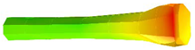 | 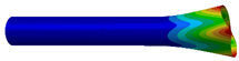 |
| 3 |  |  |
| 4 |  |  |
| 5 |  | 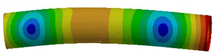 |
| 6 |  |  |
| 7 |  | 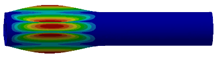 |
Publisher’s Note: MDPI stays neutral with regard to jurisdictional claims in published maps and institutional affiliations. |
© 2022 by the authors. Licensee MDPI, Basel, Switzerland. This article is an open access article distributed under the terms and conditions of the Creative Commons Attribution (CC BY) license (https://creativecommons.org/licenses/by/4.0/).
Share and Cite
MDPI and ACS Style
Yu, R.; Li, S.; Liang, L.; Liu, F.; Wang, K. Research on Stiffness Identification Method for Complex Joints Based on Modal Correlation Analysis. Machines 2022, 10, 993. https://doi.org/10.3390/machines10110993
AMA Style
Yu R, Li S, Liang L, Liu F, Wang K. Research on Stiffness Identification Method for Complex Joints Based on Modal Correlation Analysis. Machines. 2022; 10(11):993. https://doi.org/10.3390/machines10110993
Chicago/Turabian StyleYu, Ruijiang, Shujuan Li, Lie Liang, Feilong Liu, and Kaixuan Wang. 2022. "Research on Stiffness Identification Method for Complex Joints Based on Modal Correlation Analysis" Machines 10, no. 11: 993. https://doi.org/10.3390/machines10110993
Note that from the first issue of 2016, this journal uses article numbers instead of page numbers. See further details here.