
Speed-Sensorless Control of Induction Machines with LC Filter for Geothermal Electric Submersible Pumping Systems


Department of Electrical Engineering and Information Technology, Hochschule München University of Applied Sciences, Lothstr. 64, 80335 Munich, Germany
*
Author to whom correspondence should be addressed.
†
The authors contributed equally to this work.
Machines 2022, 10(2), 87; https://doi.org/10.3390/machines10020087
Submission received: 20 December 2021
/
Revised: 19 January 2022
/
Accepted: 21 January 2022
/
Published: 25 January 2022
(This article belongs to the Special Issue Feature Papers to Celebrate the First Impact Factor of Machines)
Abstract
:A speed-sensorless state-feedback controller for induction machines (IMs) with LC filter is proposed. The speed and state estimation is based on a speed-adaptive observer, requiring only the measurement of the filter input currents. The motor currents are controlled by a state-feedback controller with prefilter and integral control action, in order to achieve fast and asymptotic set point tracking. Observer and controller gains are calculated offline using linear quadratic regulator (LQR) theory and updated online (gain-scheduling) in order to attain stability and improve controller performance in the whole operation range. Implementation aspects, such as discretization of the control system and reduction of computational effort, are taken into account as well. The proposed control scheme is validated by simulations and experimental results, even for critical operating conditions such as speed zero-crossings. It is shown that the overall control system performs very well under various load- and speed conditions; while its tuning remains simple which makes it attractive for industrial application such as geothermal electric submersible pumping (ESP) systems.
1. Introduction
In medium-voltage (MV) variable-speed drive applications with long power cables such as geothermal electrical submersible pumping (ESP) systems [1], an inverter output (load) LC filter is often employed between voltage source inverter (VSI) and induction machine (IM) as to (i) decrease voltage deflection at the motor terminals, due to impedance imbalance between the cable and the motor, and to (ii) reduce steep voltage slopes which might damage the motor insulation and bearings due to high capacitive discharge [2,3,4]. However, the additional hardware comes at cost of electric coupling between the filter and motor currents and voltages, respectively, which in turn complicates the design of the control system. Although the filter capacitance and inductance are typically selected such that the resonance frequency is located in the frequency band between the rated fundamental frequency and the inverter switching frequency [2], the filter capacitance may lead to self-excitation of the induction machine within the operational frequency band [1].
Figure 1 shows magnitude and phase plots (assuming constant slip conditions) of the transfer functions from the filter output voltage to the filter current and stator current , respectively. It can be seen that, in the no load case, the filter current (providing reactive power only) is heavily damped near p.u., which corresponds to the self-excitation frequency , i.e., the frequency at which reactive power is mainly exchanged between the stator inductance and the filter capacitance. Moreover, the resonance peak is identified at p.u., which corresponds to its designed value. It can be deduced from the phase plot that the filter load changes from a slightly inductive load to a predominantly capacative load in-between the two resonant peaks, while the machine load remains inductive until the filter resonant frequency is reached. In conclusion, the LC filter has a strong impact on the dynamics of the filter current and, thus, requires consideration in the control system. The cable, on the other hand, may be neglected in the control design, since its impact is negligible due to the LC filter, except for the resistive part which may be added to the stator resistance of the IM [1].
Regarding the control of IMs with LC filter, typically a system of cascaded proportional-integral (PI) or dead-beat controllers is proposed [5,6,7,8,9]. These controllers, however, require individual tuning based on heuristic tuning rules, which may be tedious and non-intuitive. Among the few publications further incorporating a speed-sensorless approach (i.e., [6,7,9]), the contribution of [6] stands out due to its minimal requirements on the measurement system, extensive stability analysis and provision of experimental results for all critical operation regimes. The method extends the (IM only) adaptive observer presented in [10] to the given electrical drive system of IM and LC filter. However, it has not been revisited ever since.
As for the standalone IM case (without LC filter), observer-based speed-sensorless control can be considered a mature research topic, which was constantly developed since it first appeared in the early nineties [11]. Ever after, main research focus has been on stabilizing the observer in the whole operation range, in particular in the low-speed regeneration mode (e.g., [10,12,13,14,15,16,17]). Recent developments of observer-based approaches are found in [18,19,20,21,22,23,24,25], including extended Kalman filter (EKF) and sliding mode observer (SMO) approaches. However, it is pointed out in [26], that in order to achieve so-called complete stability [27] (i.e., stable operation in all operation regimes except DC excitation) an analytical selection of the observer gains is essential.
The problem arises when trying to transfer the recent results from the IM only case to the extended case of IM with LC filter because the extended setup is of higher order making an analytical gain selection infeasible.
In order to circumvent the problem of manual tuning of the the full-state observer, a programmatic tuning approach is chosen in this work, i.e., by applying the well-known linear-quadratic regulator (LQR) method from optimal control theory. In order to account for the varying speed and load, gain-scheduled FSO implementation is performed. Moreover, tuning guidelines for the choice of the weighting matrices are provided, resulting in one single design parameter for the observer only. The speed adaption gains on the other hand are selected based on a linearization analysis. Additional means to stabilize the system in the low-speed regime—i.e., (i) a stator resistance adaption at low speeds, (ii) an inverter output correction (both based on [18], which is for IMs without LC filter, though) and (iii) fast observer sampling (twice per switching period)—are implemented.
As for the control system, the concept of cascaded PI controllers is replaced by a single gain-scheduled state-feedback controller (SFC), providing a unified framework for tuning and to control all system states at once. In addition, set-point tracking for the stator currents is achieved by employing a prefilter and integral control action. The feedback gains are likewise tuned using the LQR approach with heuristic guesses for the weighting matrices, leaving a total of solely three design parameters in contrast to several tuning parameters if conventional cascaded controller structures are utilized. Moreover, the inverter delay is considered in the SFC by means of two additional system states. Speed and flux, respectively, are controlled by outer PI controllers, which provide the current references for the underlying SFC.
The theoretical results are validated by comprehensive simulation and experimental results, showing a good overall match of simulations and measurements and that an excellent, robust and similar control performance as in [6] is achieved while implementation and tuning is simpler and unified.
The contributions of this work can be summarized as follows:
- a generic discretization framework for simple system and observer discretization and implementation;
- a novel LQR-based and gain-scheduled state-feedback controller (SCF) with solely three tuning parameters;
- a novel LQR-based and gain-scheduled full-state observer (FSO) with solely one tuning parameter; and
- comprehensive simulation and measurement results validating the proposed control system as simple, effective and robust alternative to available approaches in literature in the whole speed and torque range.
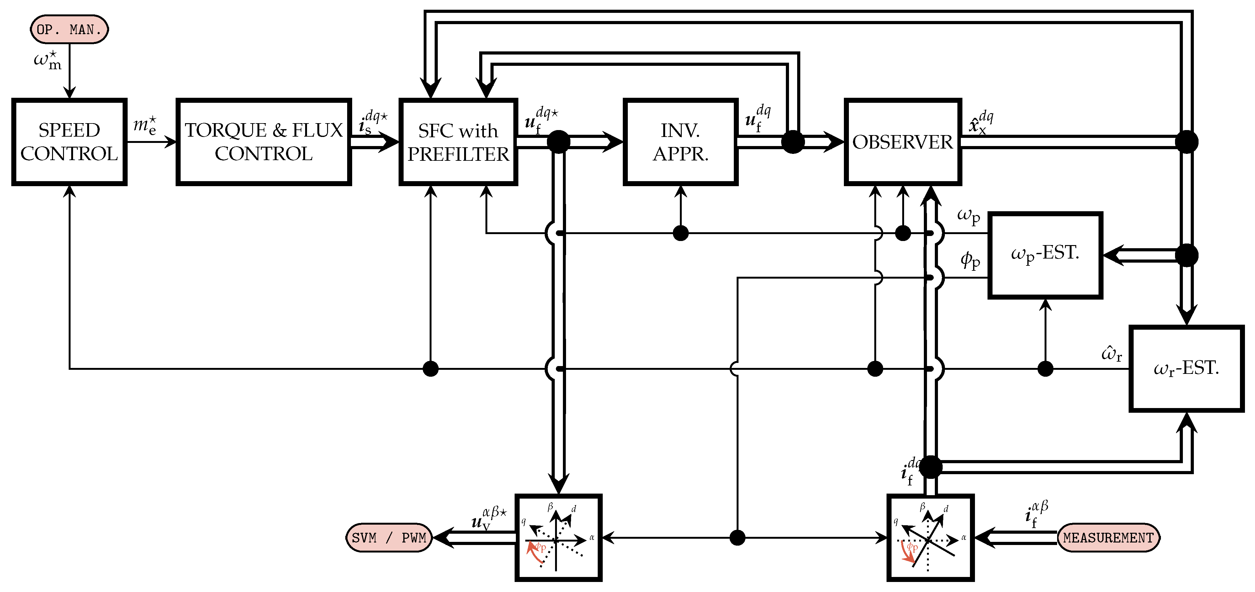
The outline of the remainder of the paper is illustrated in Figure 2 as overview block diagram of the complete system consisting of physical system [---] (see Section 2), the observer system [---] (see Section 3) and the control system [---] (see Section 4). The proposed overall control system including FSO, SFC and outer speed/torque controller is implemented and validated by simulations and measurements in Section 5. Section 6 summarizes the results of this paper and gives a short conclusion.
2. Description and State Space Model of Physical System
The complete electrical drive system is depicted in the upper part of Figure 2 (physical system). However, only the following components are considered in the drive model:
- (i)
- Voltage source inverter (VSI),
- (ii)
- inverter output filter (LC filter) and
- (iii)
- three-phase squirrel-cage induction machine (IM).
The VSI produces modulated phase voltages at its ouput terminals (according to the implemented modulation scheme). The phase currents flow from the inverter output to the LC filter input. The LC filter output is in turn connected to the machine terminals. The (filtered) stator voltages drive the stator currents . Due to magnetic coupling between stator and rotor of the machine, the induced voltages in the rotor windings (cage) produce currents resulting in the rotor flux linkage . The IM rotates at mechanical angular velocity , which is proportional to the electrical angular velocity with number of IM pole pairs. The produced electromagnetic torque is denoted by (load torque and friction torque act against ).
In Figure 2, all electrical quantities of the real system (upper part) are given in three-phase -coordinates. However, the modeling and control (lower part) will be conducted using space vector notation in the rotating -reference frame which is aligned with the rotor flux linkage (details are omitted), i.e., applying Clarke and Park transformation to all quantities above leading to with (for details see [28] [Chapter 14]). Hence, the -reference frame rotates at synchronous speed and is displaced by the angle from the stationary -reference frame.
The following assumptions (An) are imposed on the system:
- (A1)
- Magnetic saturation is negligible and flux linkages depend linearly on the currents, i.e.,
- (A2)
- Quasi-constant speed: The mechanical system is significantly slower than the electrical system and, hence, can be considered a slowly time-varying parameter.
- (A3)
- Quasi-constant load: The load torque is a slowly varying disturbance and, hence, the synchronous speed becomes a slowly time-varying parameter, too.
- (A4)
- Measured quantities: Only dc link voltage and filter (input) currents are measured and available for feedback.
2.1. Continuous-Time (CT) System Description
Based on Assumptions (A1)–(A4), the dynamics of IM and LC filter can be derived in the rotating -reference frame as (see [1])
where and are the system state vector and output, resp., and
denote the system matrix (), input matrix (), output matrix (), resp., and is a block matrix with matrices as block diagonal elements. The subscript of the system matrix indicates that states x act on states x, whereas e.g., means that inputs u act on states x (will be used later). Moreover, and are the filter, stator and rotor time constants; and are the filter inductance, capacitance and series resistance; , , , and are the stator and rotor self inductances, the main inductance and the stator and rotor leakage inductances; is the leakage coefficient; and are the stator and rotor resistances and is an auxiliary inductance term (for details, see [1]).
2.2. Generic Discrete-Time (DT) System Description
Since low switching frequencies are used in medium-voltage applications, observer and controller design in the discrete domain is mandatory and yields a better and more robust implementation. Assuming a zero-order hold (ZOH) input and sampling time , the discrete time system is given by
with and discrete system matrices
Calculation of the exact matrix exponential requires , which is typically approximated by chosing a finite value for N. Moreover, by introducing the matrix , calculating the inverse of is circumvented. Note that yields the simple forward Euler discretization method, which is known to cause stability issues at lower sampling frequencies. Therefore, it is recommended to chose .
3. Observer System
The observer system is depicted in the bottom right part of Figure 2 and combines various subcomponents, which each contribute to reproducing the actual system state. Given the low switching frequencies in medium-voltage (MV) drives, the observer is sampled at a higher rate , using buffered measurements of the filter currents and reconstructed mean voltages.
3.1. Oversampling and Voltage Reconstruction
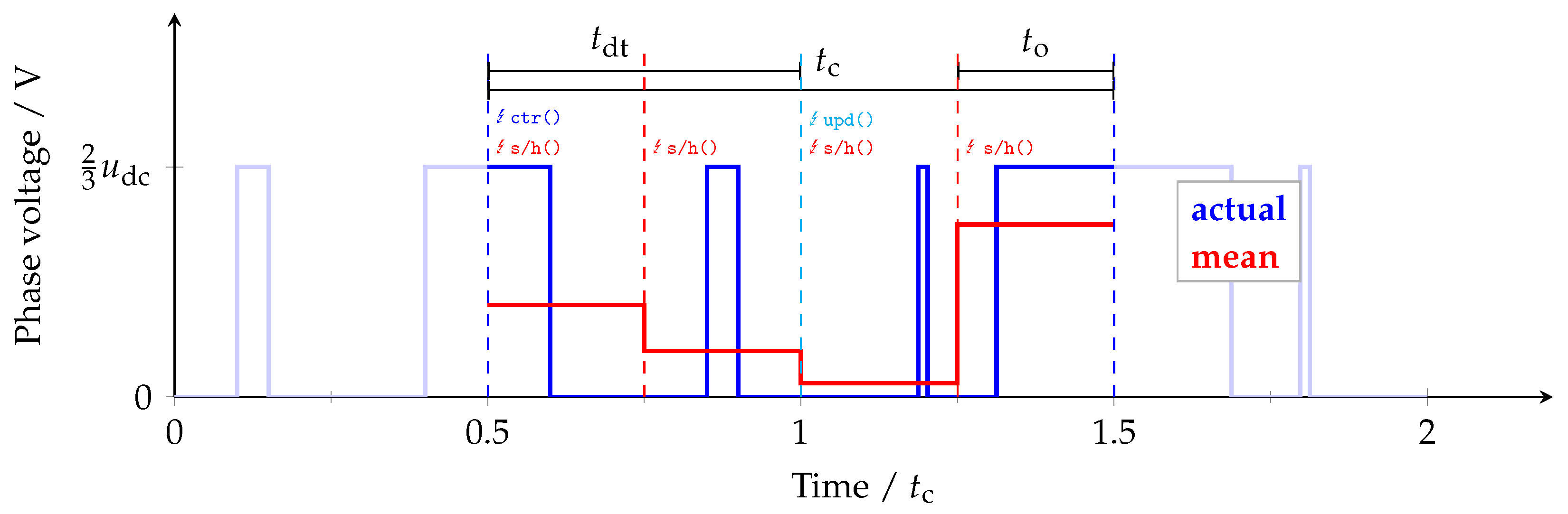
Eventhough typical switching frequencies for MV drive applications do not exceed 1 , the analog-to-digital conversion (ADC) sampling rate can be chosen higher, with denoting the oversampling factor. The ADC results are stored in a buffer of size M, i.e., for example, the filter current buffer and the DC link voltage buffer , and emptied upon control routine excecution. Using the filled measurement buffers, the observer routine can be executed retroactively in a loop, with the final result representing the predicted states for the current time instant. Naturally, the loop execution requires more computation time than a single observer step, which is acceptable, though, due to the low switching frequency. Since the inverter output voltage is not measured, it must be reconstructed with the same resolution as the measurements.
The voltage reconstruction is illustrated in Figure 3. In this paper, symmetrical pulse-width modulation (PWM) with execution of the controller interrupt routine ctr() at the end of each switching period is employed, which gives an output delay of (time between calculation of the next control step and the PWM update upd()). This way, using the previous voltage command, the voltage waveform over the interval spanning from the actual to the next control step, can be reconstructed. This interval of length is subdivided into M time windows, for which the mean voltages are calculated and stored in the voltage buffer . Moreover, the sample-and-hold event s/h() is triggered for each window, such that the corresponding current and dc link voltage measurements are available. Knowledge of the modulation scheme (e.g., space vector modulation) and (buffered) measurements for allow to compute the mean voltages for each subinterval yielding precise inputs for the observer.
3.2. Luenberger Observer with Gain-Scheduling
Assuming perfect parameter knowledge—except for the mechanical speed —the discrete-time Luenberger observer is given by
with observed states , outputs , state error and (estimated) speed-dependent discrete system, input and observer gain matrices and , respectively. The observer has two inputs, namely the inverter output voltage and the state error . Since the angular velocity is not measured, the observer system matrix depends on the speed estimate , which in turn propagates into the input matrix due to the discretization (only for ). Note that the sampling time for the calculation of the discrete-time system matrices in (6) according to (5) is selected as for the observer.
Most publications dealing with speed-adaptive observers for induction machines focus on the selection of feedback gains by pole placement, in order to achieve stable operation over a wide operation range (see e.g., [17,29]). In this paper, a programmatic approach is chosen, which is based on the well-known linear quadratic regulator (LQR) theory, in combination with the concept of gain-scheduling as to account for the time-varying parameters and . It can be shown that for sufficiently large N (discretization order) and small sampling time , the error difference can be approximated as
where
and is the speed estimation error. Details on the derivation can be provided by the authors upon request.
For the feedback gain calculation, a zero speed-estimation error is assumed, i.e., . The objective is to find a feedback gain matrix , such that the error difference is asympotically stable, and, hence, the state error converges to zero (i.e., all eigenvalues are located inside the unit circle of the complex plane). Since the eigenvalues of are equal to the eigenvalues of its transpose (dual system), finding the optimal observer gain matrix can be reduced to a control problem.
The objective of the LQR approach is to find the feedback gain matrix , for which the control law minimizes the quadratic cost function
where and are the state and input vectors of the respective dual system, is a positive (semi)-definite symmetric state weighting matrix and is a positive definite symmetric input weighting matrix. The optimal solution is given by , where the matrix is the infinite horizon solution of the discrete-time Ricatti equation (for details see Section 10-8 in [30]). The solution of the LQR problem is calculated by software (e.g., in MATLAB with the dlqr(...) command). The weighting matrices, can be chosen in the following simple manner: (i) Use diagonal matrices for and , (ii) normalize the diagonal elements with respect to the rated (nominal) state or input variables (subscript ‘R’) and (iii) introduce a weighting factor to prioritize state weighting matrix or input weighting matrix . The following weighting matrices
are chosen. Note that the only tuning factor is , which makes the observer design a straight forward and simple task.
Due to the fact that the system matrix depends on the parameters and , the observer gains are adapted online, i.e., holds. This is achieved by offline calculation of the observer gains using the LQR method for several (but constant) values of and and storing the results in individual look-up tables (LUTs). During operation, the gains are updated in each sampling instant using 2D linear interpolation based on the new values of and .
Remark 1.
In order to improve computation and data efficiency, the quasi-complex property of the gain matrix can be exploited, i.e., each 2-by-2 gain block can be written as for gain blocks and representing quasi-real and quasi-imaginary part. This way, only half of the entries of need to be stored in and extracted from the LUT.
3.3. Speed Adaption
Typically, a PI-controller is used for the online adaption of the speed estimate (e.g., [6,10,15]). Input to the controller is the “error torque” , resulting from the IM stator current estimation error and the rotor flux linkage estimate . However, since only the filter currents are available for feedback [see Assumption (A4)], a different input to the PI-controller is needed. Salomäki et al. [6] were the first to propose the use of a slightly different error torque
depending on the filter current estimation error (instead of ) and , leading to the adaption law
with proportional gain and integral gain .
Remark 2.
The gains and have a significant impact on the observer stability and must be chosen with care. To do so, the linearization analysis as proposed in [18] for IMs only (i.e., without LC filter) has been extended and conducted for the IM+LC system here. It allows to find valid combinations, which guarantee local stability if good parameter knowledge is assumed. For this work, such analysis has been conducted. However, in practice it was found that a purely integral adaption law constitutes the most robust solution.
Steady-state (indicated by ) analysis of the state estimation error —i.e., by setting or and solving (7) for —shows that the current error substitution is indeed feasible. The steady-state error torques are given by
with speed dependent “constants” and . Calculating both constants numerically (e.g., with parameters in Table 1) for different values of and , reveals that (see Figure 4). Clearly, small deviations are observed, yet no switch of sign occurs and, as a consequence, using the filter current error for the speed adaption is a viable alternative.
3.4. Flux Angle Detection
For rotor flux linkage orientation of the rotating -reference system, the speed of the synchronously rotating reference frame and the respective angle have to be defined. By assuming that the entire flux linkage is concentrated in the d-component, it follows that and . Hence, the flux linkage dynamics of the q-component can be solved for , yielding
3.5. Stability of the Observer
Stability proofs of speed-adaptive observers have extensively discussed in literature, since a first observer was used for induction machines by Kubota et al. [11] in the early nineties. Kubota tried to prove stability using a Lyapunov function yielding a simple integral adaption rule. However, the proof neglected an immeasurable flux term which weakens its validity. At the same time, other authors—e.g., Schauder [31] and Yang [32]—tried to prove stability using the concept of hyperstability. As pointed out by e.g., Suwankawin [33] in 2002, their proofs were wrong. In 2007, Sangwongwanich et al. were, as the first, able to provide a proof for complete stability under strict conditions on the observer gains [17]. Harnefors and Hinkkanen used a different approach to proof complete stability, by using a linearization approach [29]. To conclude: Proving complete stability is considered to be solved under strict conditions but not in general. Nevertheless, since the focus of this work is on the overall state-feedback control system and not on a rigor stability proof, the authors refer to earlier publications by e.g., Salomäki [6] and to the experimental and simulative validation as a proof of concept.
4. Control System
The control system is depicted in the lower left part of Figure 2. A classical PI-speed controller is used to control the machine speed by passing a torque reference to the underlying feed-forward torque controller. The torque controller translates the torque set point into stator current setpoints. Finally, the state-feedback controller actively controls the stator currents in compliance with the given set point values, while the remaining system states are controlled indirectly. Instead of using and tuning several cascaded PI controllers (as e.g., in [6]), the proposed state-feedback controller tuning is straight forward. Employing the LQR tuning method ensures a simple design process and requires only three tuning parameters (see Section 4.3.4). Moreover, (overall) closed-loop stability is guaranteed.
4.1. Proportional-Integral Speed Controller with Anti-Windup
In view of the limited machine torque available, the considered PI-controller is implemented with anti-windup and is given by the following control law (see Section 10.4.1 in [28])
with proportional and integral gains, integrator output and control error . The anti-windup decision function (conditional integration)
disables integration in (16) when the absolute value of the machine torque set point exceeds the maximally available IM torque to suppress windup effects. Tuning of the gains and can be done e.g., by using analytical methods like the symmetrical optimum criterion (see Section 4.4.4 in [34]).
4.2. Feed-Forward Torque Controller and Rotor Flux Controller
The reference torque can be mapped to a pair of stator current set points and . Typically, in the non-field weakening operation regime, a constant flux is used, i.e., the d-component of the stator currents is fixed to its nominal value, whereas the q-component is used to realize the given torque reference. The motor torque can be stated as
Hence, for estimtated rotor flux linkage and given torque reference , the q-current reference becomes
whereas the the d-current reference is obtained as output from the rotor flux linkage PI-controller
with proportional and integral gains, integrator output and flux linkage control error . The anti-windup decision function is similar to (17) with maximum admissible d-reference current as treshold (instead of ) and disables integration in (20). Tuning of the gains and can be done e.g., by the magnitude optimum criterion, see Section 4.4.4 in [34].
4.3. State-Feedback Control of the Drive System
A state-feedback controller is designed which controls all system states simultaneously. Instead of using and tuning several and cascaded PI-controllers (as e.g., in [6]), the state-feedback controller tuning is simple and holistic. Employing the well-known LQR tuning method in combination with gain-scheduling ensures an easy design process and guarantees (overall) closed-loop stability. Control objective is reference tracking of the stator currents of the electric machine and suppression of oscillations in the remaining system states (due to the LC filter). Based on the Separation Principle (see e.g., Chapter 8.4 in [35]), the controller is designed for system (4); assuming all states are available for feedback. Once the controller is derived, controller and observer are merged and implemented altogether.
4.3.1. Discrete-Time Inverter Approximation
The VSI produces the modulated output voltage according to the reference vector by pulse width modulation (PWM). This output voltage generation comes with a time delay (see Figure 3), which depends on the employed modulation scheme and is inversely proportional to the switching frequency of the inverter.
For MV drive applications, typically a low switching frequency is used, which increases the time delay and thus necessitates its consideration in the model. Formalizing the ideas of Figure 3 for the case (switching frequency equals sampling frequency of the controller), the discrete-time inverter model can be stated as
where the new state is the back-rotated version (inverse Park transform with argument ) of the previous time step filter reference voltage. Moreover, the (partial) input matrix determines the impact of the input on the state . For the sake of simplicity, it is assumed in the following that the switching delay equals the (controller) sampling time, i.e., holds. As a consequence, the inverter voltage becomes equal to the inverter state, i.e., , and (21) simplifies to
4.3.2. Continuous-Time Augmented System
The classical state-feedback controller does not allow for tracking of state reference values. Therefore, a new input is defined, which represents the set point vector of the stator currents. Note that, since the system has two inputs only, merely two states can be controlled independently.
In order to ensure asymptotic set point tracking, i.e., , the system is extended by two additional integrator states which represent the respective integrals over the state tracking errors. The dynamics of the new states are defined as
where selects the stator currents from the state vector .
Finally, the overall augmented system is given by
where and are the augmented state vector and control output, resp., and
are the augmented system matrix , input matrix , set point matrix and control output matrix .
For implementation and controller tuning, this system must be discretized with the controller sampling time by invoking (5). The details are omitted as this step is straight forward. However, the resulting discrete-time matrices
with respective partitioning, will be used in the following. The discrete-time integral error system which is required for the controller implementation can now be stated as
4.3.3. Overall Discrete-Time System
Finally, the overall discrete-time system can be constructed from the partial results of the previous steps, i.e.,
The new control input is (instead of ), i.e., a control law using is to be found.
4.3.4. State-Feedback Control Law with Prefilter
Since the augmented system (28) is fully controllable, a state-feedback controller of the following form can be designed
with feedback gain matrix , and where , and . Moreover, using the gain matrix a feedforward term or prefilter is introduced.
Similar to the observer gain selection, the controller gain matrix is calculated using the (discrete) LQR approach with the following weighting matrices
The factor in constitutes an additional tuning factor, weighting the integral-action. It is important to note, that for the SFC, solely two parameters (i.e., and ) must be tuned.
In analogy to the observer, gain-scheduling is used, i.e., the controller gains are updated in each control cycle. Therefore, the LQR algorithm has to be repeated offline for several combinations of and , yielding 2D LUTs for each entry of and, hence, holds. Note that, as for the observer gains, only half of the gains need to be stored and looked-up during operation.
4.3.5. Prefilter Calculation
It remains to determine the prefilter gain matrix , which allows for faster set-point tracking by supporting the integral part of the controller. The idea is to anticipate the required voltage for a given stator current reference by evaluating the steady-state equation
which can be solved for . Note that the steady-state integral error cannot be known a-priori (otherwise it would not be needed), so that only the inverter and the IM + LC systems are considered in the equation, while the integral action states are left out. The solution to (31) is given by (details are ommitted due to lengthy derivation)
where the submatrices and are obtained from partitioning and , accordingly. Finally, an additional tuning factor is introduced, which allows to reduce the impact of the feedforward control action (if necessary), i.e.,
This has proven useful in practice, as the sensivity to modeling and parameter errors is reduced and, hence, large overshooting can be avoided. Note that depends on and , which requires its recalculation in each control step or the use of an additional LUT. Although the equation can be greatly simplified using symbolic calculations (many zero entries), using gain-scheduling for the 2-by-2 feedforward gain matrix is advisable as the solution of the inverse of a 10-by-10 matrix is usually computationally expensive.
4.3.6. Output Saturation
Since the output voltage of the VSI is constrained, the controller output must be limited, too. Therefore, the magnitude of the reference voltage is limited by
where the maximum voltage depends on the dc-link voltage and the employed modulation scheme (e.g., for space vector modulation, holds). The saturated output is passed on to the modulator.
4.4. Implementation of the Control System
For the implementation of the overall system, observer and control system are implemented independently of each other, as both potentially use different sampling times and , respectively. The observer is realized according to (6), with speed estimation (12) and estimated rotor flux orientation (15). The estimated states and speed , as well as the electrical frequency , are fed to the control system, which only needs to realize the inverter delay (22) and the integral error system (27). By looking up the controller gains, depending on the current values of and , the control output can be calculated. The reference voltage, in turn, is used by the observer to reconstruct the voltage input.
Lastly, an overview of the complete system with speed-adaptive observer, state-feedback controller and speed & torque controller is shown in Figure 5.
5. Experimental and Simulative Validation
In this section, simulative and experimental validation of the proposed control scheme are shown for a system described by the parameters given in Table 1. Since the controller is supposed to run on a digital signal processing (DSP) unit, the derived control system is discretized. The implementation itself is done in MATLAB and Simulink R2017a for both, simulation and experiment. The simulation environment, as well as the experimental setup are briefly described. Finally, the results are discussed and evaluated.

Table 1.
Parameters of the test setup.
| Parameter | Variable | Value | Unit | |
|---|---|---|---|---|
| VSI | DC-link voltage | 580 | ||
| Switching frequency | 4000 | |||
| Filter | Rated current (amplitude) | 22 | ||
| Inductance | 4.5 × 10⁻³ | |||
| Capacitance | 30 × 10−6 | |||
| Resistance | 0.1 | |||
| Induction machine | Rated speed (nameplate) | 298.4 | rad s−1 | |
| Rated torque | 10.05 | |||
| Rated voltage (amplitude) | 327 | |||
| Rated current (amplitude) | 8.1 | |||
| Rated power factor | 0.93 | 1 | ||
| Rated flux (amplitude) | 1.2 | |||
| Number of pole pairs | 1 | 1 | ||
| Stator resistance | 1.85 | |||
| Rotor resistance | 1.55 | |||
| Main inductance | 340 × 10−3 | |||
| Stator leakage inductance | 16.5 × 10⁻³ | |||
| Rotor leakage inductance | 16.5 × 10⁻³ | |||
| Control system | P-gain (speed estimator) | 0 | rad s−1 N−1 m−1 | |
| I-gain (speed estimator) | 1500 | rad s−2 N−1 m−1 | ||
| P-gain (speed control) | 0.42 | N m s rad−1 | ||
| I-gain (speed control) | 10.43 | N m rad−1 | ||
| P-gain (flux control) | 26.7 | H −1 | ||
| I-gain (flux control) | 670 | H −1 s−1 | ||
| 1. weighting factor (obs.) | 1.2 × 10⁻⁸ | 1 | ||
| 1. weighting factor (contr.) | 0.5 | 1 | ||
| 2. weighting factor (contr.) | 1 × 10⁴ | 1 | ||
| 3. weighting factor (contr.) | 0.3 | 1 |
5.1. Simulation
The control system is implemented as a discrete block in Simulink, triggered at the center of each PWM period, just as in the experimental setup. The two-level VSI is supplied by a constant DC-link voltage, while the switching signals are generated using space-vector modulation (SVM). The LC filter and the (linear) induction machine are simulated based on model (2), while continuous-time integrators are used to solve the first-order differential equations. Moreover, a simplified mechanical model with viscous friction and arbitrary load torque is used. The fixed-step solver ode3 runs with a sampling time of 100 .
5.2. Experimental Setup
The testbench (see Figure 6) comprises a 3 induction machine and load machine, both equipped with position encoders, a torque sensor, a custom-built LC filter, 2-level VSIs and the dSPACE real-time system.The modular dSPACE system runs on a DS1007 processing unit, with a DS5101 module for the PWM generation, a DS2004 A/D module, and a DS3002 encoder board. Note that, unlike stated in the beginning of this chapter, stator currents, voltages and rotor speed are measured here. However, this data is only used for evaluation; it is not fed back to the control system.
5.3. Results & Discussion
To validate the proposed control and observer systems, a 60 s experiment (see Figure 7, Figure 8 and Figure 9) has been conducted which includes four critical Scenarios ()–() besides start-up and transition phases in order to show stability, functionality and performance of the closed-loop system under various speed and loading conditions in one realistic run:
- Scenario (S1)—Speed reversal (t ∈ [4 s–24 s]): In the first scenario, A speed reversal is performed under full load in order to evaluate the low speed performance of the closed-loop system. It is well-known that observability of electrical machines is lost at standstill (i.e., ). For induction machines, it is lost at zero excitation, i.e., , which occurs twice during the test and makes it most critical and crucial for validation in order to judge robustness of the speed-adaptive observer in terms of its zero-crossing capabilities.
- Scenario (S2)—Standstill (t ∈ [28 s–38 s]): The second scenario covers a standstill test under varying load. After a short period of full load, the load is ramped down slowly to zero. This test is conducted in order to evaluate and proof the low-speed capabilities of the closed-loop system at complete standstill and varying loads.
- Scenario (S3)—Field weakening (t ∈ [39 s–45 s]): In the third scenario, the high-speed capabilities of the closed-loop system are validated by performing a no-load acceleration from 0 rad s−1 to . After a short interval of high-speed operation, the speed is reset to standstill by means of active braking (generating mode). For a constant magnetic field, the induced voltage increases almost linearly with the speed, such that for rated excitation the voltage limit is reached for rated speed and load. Therefore, the magnetic field (rotor flux linkage) needs to be decreased in order to reach higher speeds than rated speed.
- Scenario (S4)—Load variations (t ∈ [47 s–59 s]): For the fourth scenario, step-like load variations disturb the closed-loop system while the speed must be kept constant at its rated value. Besides operation near the voltage limit which potentially triggers the anti-windup strategy (coniditional integration) of the integral control actions, the full controller bandwidth is evaluated and validated. The last scenario can be considered as typical (conventional) mode of operation in real-world ESP systems.
The validation results of the closed-loop system consisting of LC filter, IM and discrete implementation of observer and control system include measurement and simulation data and are shown in Figure 7, Figure 8 and Figure 9; whereas system data and tuning parameters are listed in Table 1. A detailed discussion of the results follows in the two next subsections. In the figures, the different phases (time intervals) and Scenarios ()–() are seperated by vertical lines [- - -] and shaded areas, respectively. Since the flux linkages could not be measured, either the estimated and/or simulated values are shown in the respective plots.
5.4. Experimantal Validation of the Control System
Figure 7 shows the experimental results which allow to evaluate the performance of the control system using the measured filter currents , the estimated stator currents , the estimated stator (capacitor) voltages and the estimated mechanical angular velocity as feedback. Measured (sampled) data is plotted as solid blue lines [—], whereas references and constraints (voltage limit) are drawn as dashed [▪ ▪ ▪] and dotted [▪▪▪▪▪▪] red lines, respectively. In the top-most first subplot, the timeseries of the mechanical speed and its estimate [—] are shown. Both do track the reference speed [▪ ▪ ▪] almost perfectly for all four Scenarios Scenarios ()–(). The speed rise-time is only limited due to the torque (current) limit of the IM. However, as visible in particular during the fast but ramp-like accelerations in Scenario () or during the transition phase between Scenarios () and (), the rated torque is not fully needed for accelaration as the reference speed is low-pass filtered and, therefore, less steep. For geothermal ESP systems, very fast speed changes are not admissible nor advisable which motivates the reference speed filtering. In the second subplot, the corresponding (measured) machine torque is plotted. The torque of the speed-controlled IM is equal to the overall load and acceleration torque; including friction. It can be seen that the control system is able to follow the reference torque with high accuracy. Minor deviations are only observed during standstill operation (i.e., Scenario ()) The oscillations around 27 s are due to the elastic behavior of the torque sensor which is excited by the step-like speed change. The third and fourth subplots show the estimated stator currents and and their respective set points and as outputted by flux and speed controller. Again, all references can be tracked very well by the control system. The -currents changes within a band of about 0.2 p.u. only, the -current (being proportional to the torque) varies between 1.25 times negative to positive rated stator current of the IM. The factor of 1.25 has been set as upper limiting factor for the speed controller output. The estimated rotor flux linkage is shown in the fifth subplot. As a flux controller is utilized, the flux linkage set-point is mostly constant and, only during Scenario () (field weakening), it must be reduced. The commanded set-points are nicely tracked by the control system for all four Scenarios ()–(). The bottom-most (last) subplot shows the magnitude of the filter voltage reference (VSI voltage command) and the respective voltage limit [▪▪▪▪▪▪] depending on the measured (and varying) DC-link voltage . As expected, the required voltage is close to its threshold only for higher speeds. Field weakening in Scenario () proves to be feasible and works properly as the voltage limit is not exceeded. Generative braking from 1.5 times rated speed to standstill results in a steep but only temporarily rise of the DC-link voltage , until the resistive chopper braker in the VSI becomes active. Also, for rated (motor) torque and rated speed in Scenario (), the voltage limit is (almost) reached. Nevertheless, the load changes do not perturb the system seriously and constant (rated) speed operation is assured. In conclusion, the control performance of the closed-loop system consisting of observer and control system is very acceptable and satisfactory. It is robustly stable and is able to track the references with (very) high accurary for all four scenarios.
5.5. Experimantal and Simulative Validation of the Observer System
The observer performance over the whole experiment including all four scenarios is illustrated in Figure 8, showing the evolution of the system and observer states, and Figure 9, showing the evolution of the speed estimation error. In both figures, experimental [—] and simulation [—] results are presented.
In Figure 8, the - and -components of filter currents, stator voltages, stator currents and rotor flux linkages are shown from top to bottom. The measured states are plotted as solid red [—] (simulation results) and solid blue [—] (experimental results) lines, whereas the estimated states are plotted as dashed red [▪ ▪ ▪] (simulation results) and dashed blue [▪ ▪ ▪] (experimental results) lines. As the rotor flux linkage can not be measured during the experiment, the respective time series are missing in the respective subplots.
The core objective of the observer system is to estimate all physical system states correctly, i.e., (see Figure 8 and (see indirectly Figure 9). Comparing the measured [—] and estimated [▪ ▪ ▪] states in Figure 8, it can be seen that for almost all transition intervals and scenarios a (very) good match between eastimated and real quantitites is achieved by the observer. Slight devations for and filter currents (see first and second subplots) occur in particular during Scenario () & () which is due to the critical non-observability condition close or at standstill. The estimation performance for the and stator currents (see fifth and sixth subplots) is similar to that of the filter currents. the and stator voltages (see third and fourth subplots), the estimation errors are (very) small for lower speeds, but increases slightly in the -component at higher speeds; i.e., during Scenarios () and (). The estimation of the and rotor flux linkages (see seventh and eighth subplots) can only be evaluated using simulation results (as the flux linkage was not measured). As expected due to lack of observerability, zero speed and non-zero load conditions during Scenarios () and () are more problematic for the rotor -flux linkage estimation. Nevertheless, the overall closed-loop system never becomes unstable and is capable of robustly estimating all states with good to very good accuracy.
Besides, a very good match between simulation and measurement data was achieved which underpins the quality of the model. Solely, the filter and stator currents do not match nicely in particular for Scenarios () & () which can be explained by the simplified magnetic model (neglecting saturation) used for the simulations.
Finally, in Figure 9, the speed estimation performance is shown. First note that the speed estimation error never exceeds ±2–2.5% of the rated angular velocity which shows the (very) high estimation accuracy for all four scenarios (including standstill and low speed operation). Most, peak-like but short deviations occur during transient conditions (transisition phases between differeent scenarios). As expected, highest and longest deviations occur during the critical Scenarios () & (). The slight mismatch between simulation and experimantel speed estimation error can again be traced back to the simplified magnetic model of the IM used for simulations.
6. Conclusions
A speed-sensorless state-feedback control system for an induction machine with LC filter for geothermal electric submersible pumping systems has been derived. The control system can be utilized for a wide range of high/medium-voltage applications with long cables where an LC-filter is mandatory to (i) minimize bearing life time (common mode voltage reduction) and (ii) to eliminate high dv/dt, overvoltages, cable ringing or motor overheating (due to converter induced harmonic content). Example applications are pumps, conveyors, compressors, elevators or cranes. The validity of the speed-sensorless state-feedback control system with state-feedback observer was verified in simulations and experiments, which showed a good overall match, and decent and robust controller and observer performance. The main advantage of the presented approach is its easy implementation, including a tuning approach, which relies on well-known methods (e.g., LQR) and requires only four tuning parameters (one for FSO and three for SCF). For implementation, clear guidelines for tuning (e.g., weighting factor selection) and discretization have been provided. For larger systems and lower sampling times, it might be recommendable to use an even higher degree of discretization, which, however, can easily achieved with the help of the proposed framework in this paper. Future work comprises stability improvements in the zero-speed range and incorporation of a nonlinear flux linkage model (covering saturation effects) in order to improve the angle, current and flux linkage estimation even further.
Author Contributions
Conceptualization, J.K. and C.M.H.; Data curation, J.K.; Formal analysis, J.K. and C.M.H.; Funding acquisition, C.M.H.; Investigation, J.K. and C.M.H.; Methodology, J.K. and C.M.H.; Project administration, C.M.H.; Resources, J.K. and C.M.H.; Software, J.K.; Supervision, C.M.H.; Validation, J.K. and C.M.H.; Visualization, J.K.; Writing—original draft, J.K.; Writing—review & editing, J.K. and C.M.H. All authors have read and agreed to the published version of the manuscript.
Funding
This research was funded by the Bavarian State Ministry of Education, Science and Arts during the research project “Geothermie-Allianz Bayern 1.0 & 1.5”.
Institutional Review Board Statement
Not applicable.
Informed Consent Statement
Not applicable.
Conflicts of Interest
The authors declare no conflict of interest. The funder had no role in the design of the study; in the collection, analyses, or interpretation of data; in the writing of the manuscript, or in the decision to publish the results.
Abbreviations
The following abbreviations are used in this manuscript:
| ADC | Analog-to-Digital Conversion |
| DSP | Digital Signal Processor |
| SFC | State-Feedback Controller |
| FSO | Full-State Obserer |
| LQR | Linear Quadratic Regulator |
| IM | Induction Machine |
| PI | Proportional-Integral (controller) |
| VSI | Voltage Source Inverter |
| MV | Medium-Voltage |
| PWM | Pulse Width Modulation |
| SVM | Space Vector Modulation |
Notation
: natural, real numbers; : column vector, where “” and “” mean “transposed” and “is defined as”, resp.; : scalar product of vectors & ; : Euclidean norm of ; : matrix (n rows & columns); , : inverse, inverse transpose of (if exist), resp.; : identity matrix; : zero vector; : zero matrix; : Park transformation matrix with & (Park transformation angle and angular velocity, respectively); : rotation matrix (by ); , or : estimates of quantities, vectors or matrices for observer design.
Remark: All physical quantities are introduced and explained in the text to ease reading.
References
- Kullick, J.; Hackl, C.M. Dynamic Modeling and Simulation of Deep Geothermal Electric Submersible Pumping Systems. Energies 2017, 10, 1659. [Google Scholar] [CrossRef] [Green Version]
- Liang, X.; Kar, N.C.; Liu, J. Load filter design method for medium voltage drive applications in electrical submersible pump systems. IEEE Trans. Ind. Appl. 2014, 51, 2017–2029. [Google Scholar] [CrossRef]
- Abu-Rub, H.; Bayhan, S.; Moinoddin, S.; Malinowski, M.; Guzinski, J. Medium-Voltage Drives: Challenges and existing technology. IEEE Power Electron. Mag. 2016, 3, 29–41. [Google Scholar] [CrossRef]
- Smochek, M.; Pollice, A.F.; Rastogi, M.; Harshman, M. Long Cable Applications From a Medium-Voltage Drives Perspective. IEEE Trans. Ind. Appl. 2016, 52, 645–652. [Google Scholar] [CrossRef]
- Kojima, M.; Hirabayashi, K.; Kawabata, Y.; Ejiogu, E.C.; Kawabata, T. Novel vector control system using deadbeat-controlled PWM inverter with output LC filter. IEEE Trans. Ind. Appl. 2004, 40, 162–169. [Google Scholar] [CrossRef]
- Salomaki, J.; Hinkkanen, M.; Luomi, J. Sensorless Control of Induction Motor Drives Equipped With Inverter Output Filter. IEEE Trans. Ind. Electron. 2006, 53, 1188–1197. [Google Scholar] [CrossRef]
- Mukherjee, S.; Poddar, G. Fast Control of Filter for Sensorless Vector Control SQIM Drive With Sinusoidal Motor Voltage. IEEE Trans. Ind. Electron. 2007, 54, 2435–2442. [Google Scholar] [CrossRef]
- Hatua, K.; Jain, A.K.; Banerjee, D.; Ranganathan, V.T. Active Damping of Output LC Filter Resonance for Vector-Controlled VSI-Fed AC Motor Drives. IEEE Trans. Ind. Electron. 2012, 59, 334–342. [Google Scholar] [CrossRef]
- Guzinski, J.; Abu-Rub, H. Sensorless induction motor drive with voltage inverter and sine-wave filter. In Proceedings of the 2013 IEEE International Symposium on Sensorless Control for Electrical Drives and Predictive Control of Electrical Drives and Power Electronics (SLED/PRECEDE), Munich, Germany, 17–19 October 2013; pp. 1–8. [Google Scholar]
- Hinkkanen, M.; Luomi, J. Stabilization of regenerating-mode operation in sensorless induction motor drives by full-order flux observer design. IEEE Trans. Ind. Electron. 2004, 51, 1318–1328. [Google Scholar] [CrossRef] [Green Version]
- Kubota, H.; Matsuse, K.; Nakano, T. DSP-based speed adaptive flux observer of induction motor. IEEE Trans. Ind. Appl. 1993, 29, 344–348. [Google Scholar] [CrossRef]
- Hofmann, H.; Sanders, S. Speed-sensorless vector torque control of induction machines using a two-time-scale approach. IEEE Trans. Ind. Appl. 1998, 34, 169–177. [Google Scholar] [CrossRef]
- Holtz, J.; Quan, J. Sensorless vector control of induction motors at very low speed using a nonlinear inverter model and parameter identification. IEEE Trans. Ind. Appl. 2002, 38, 1087–1095. [Google Scholar] [CrossRef]
- Tajima, H.; Guidi, G.; Umida, H. Consideration about problems and solutions of speed estimation method and parameter tuning for speed-sensorless vector control of induction motor drives. IEEE Trans. Ind. Appl. 2002, 38, 1282–1289. [Google Scholar] [CrossRef]
- Kubota, H.; Sato, I.; Tamura, Y.; Matsuse, K.; Ohta, H.; Hori, Y. Regenerating-mode low-speed operation of sensorless induction motor drive with adaptive observer. IEEE Trans. Ind. Appl. 2002, 38, 1081–1086. [Google Scholar] [CrossRef]
- Suwankawin, S.; Sangwongwanich, S. Design strategy of an adaptive full-order observer for speed-sensorless induction-motor Drives-tracking performance and stabilization. IEEE Trans. Ind. Electron. 2006, 53, 96–119. [Google Scholar] [CrossRef]
- Sangwongwanich, S.; Suwankawin, S.; Po-ngam, S.; Koonlaboon, S. A Unified Speed Estimation Design Framework for Sensorless AC Motor Drives Based on Positive-Real Property. In Proceedings of the 2007 Power Conversion Conference, Nagoya, Japan, 2–5 April 2007; pp. 1111–1118. [Google Scholar]
- Qu, Z.; Hinkkanen, M.; Harnefors, L. Gain Scheduling of a Full-Order Observer for Sensorless Induction Motor Drives. IEEE Trans. Ind. Appl. 2014, 50, 3834–3845. [Google Scholar] [CrossRef] [Green Version]
- Sun, W.; Yu, Y.; Wang, G.; Li, B.; Xu, D. Design Method of Adaptive Full Order Observer With or Without Estimated Flux Error in Speed Estimation Algorithm. IEEE Trans. Power Electron. 2016, 31, 2609–2626. [Google Scholar] [CrossRef]
- Wang, B.; Zhao, Y.; Yu, Y.; Wang, G.; Xu, D.; Dong, Z. Speed-Sensorless Induction Machine Control in the Field-Weakening Region Using Discrete Speed-Adaptive Full-Order Observer. IEEE Trans. Power Electron. 2016, 31, 5759–5773. [Google Scholar] [CrossRef]
- Yin, Z.; Zhang, Y.; Du, C.; Liu, J.; Sun, X.; Zhong, Y. Research on Anti-Error Performance of Speed and Flux Estimation for Induction Motors Based on Robust Adaptive State Observer. IEEE Trans. Ind. Electron. 2016, 63, 3499–3510. [Google Scholar] [CrossRef]
- Zaky, M.S.; Metwaly, M.K. Sensorless Torque/Speed Control of Induction Motor Drives at Zero and Low Frequencies With Stator and Rotor Resistance Estimations. IEEE J. Emerg. Sel. Top. Power Electron. 2016, 4, 1416–1429. [Google Scholar] [CrossRef]
- Zerdali, E.; Barut, M. The Comparisons of Optimized Extended Kalman Filters for Speed-Sensorless Control of Induction Motors. IEEE Trans. Ind. Electron. 2017, 64, 4340–4351. [Google Scholar] [CrossRef]
- Zaky, M.S.; Kamel Metwally, M.; Azazi, H.; Deraz, S. A New Adaptive SMO for Speed Estimation of Sensorless Induction Motor Drives at Zero and Very Low Frequencies. IEEE Trans. Ind. Electron. 2018, 65, 6901–6911. [Google Scholar] [CrossRef]
- Chen, J.; Huang, J. Globally Stable Speed-Adaptive Observer With Auxiliary States for Sensorless Induction Motor Drives. IEEE Trans. Power Electron. 2019, 34, 33–39. [Google Scholar] [CrossRef]
- Harnefors, L.; Hinkkanen, M. Stabilization Methods for Sensorless Induction Motor Drives—A Survey. IEEE J. Emerg. Sel. Top. Power Electron. 2014, 2, 132–142. [Google Scholar] [CrossRef]
- Hinkkanen, M.; Harnefors, L.; Luomi, J. Reduced-Order Flux Observers With Stator-Resistance Adaptation for Speed-Sensorless Induction Motor Drives. IEEE Trans. Power Electron. 2010, 25, 1173–1183. [Google Scholar] [CrossRef]
- Hackl, C.M. Non-Identifier Based Adaptive Control in Mechatronics: Theory and Application; Springer International Publishing: Berlin, Germany, 2017. [Google Scholar]
- Harnefors, L.; Hinkkanen, M. Complete Stability of Reduced-Order and Full-Order Observers for Sensorless IM Drives. IEEE Trans. Ind. Electron. 2008, 55, 1319–1329. [Google Scholar] [CrossRef]
- Ogata, K. Modern Control Engineering, 5th ed.; Instrumentation and Controls Series; Prentice Hall PTR: Upper Saddle River, NJ, USA, 2010. [Google Scholar]
- Schauder, C. Adaptive speed identification for vector control of induction motors without rotational transducers. IEEE Trans. Ind. Appl. 1992, 28, 1054–1061. [Google Scholar] [CrossRef]
- Yang, G.; Chin, T.H. Adaptive-speed identification scheme for a vector-controlled speed sensorless inverter-induction motor drive. IEEE Trans. Ind. Appl. 1993, 29, 820–825. [Google Scholar] [CrossRef]
- Suwankawin, S.; Sangwongwanich, S. A speed-sensorless IM drive with decoupling control and stability analysis of speed estimation. IEEE Trans. Ind. Electron. 2002, 49, 444–455. [Google Scholar] [CrossRef]
- Schröder, D.; Böcker, J. (Eds.) Elektrische Antriebe–Regelung von Antriebssystemen; Springer: Berlin/Heidelberg, Germany, 2020. [Google Scholar] [CrossRef]
- Goodwin, G.C.; Graebe, S.F.; Salgado, M.E. Control System Design, 1st ed.; Prentice Hall PTR: Upper Saddle River, NJ, USA, 2000. [Google Scholar]
Figure 1.
Magnitude (a) and phase (b) plots for transfer functions (blue) and (red), assuming constant slip (i.e., ). Plotted for different loads, i.e., line styles solid, dashed and dotted refer to no-load, half rated load and rated load conditions, respectively.
Figure 1.
Magnitude (a) and phase (b) plots for transfer functions (blue) and (red), assuming constant slip (i.e., ). Plotted for different loads, i.e., line styles solid, dashed and dotted refer to no-load, half rated load and rated load conditions, respectively.

Figure 2.
Components of the electrical drive system comprising power electronics, LC-filter and induction machine.
Figure 2.
Components of the electrical drive system comprising power electronics, LC-filter and induction machine.

Figure 3.
Exemplary voltage reconstruction of the partial mean voltages for oversampling factor (Please note that is often the best compromise from practical point of view).
Figure 3.
Exemplary voltage reconstruction of the partial mean voltages for oversampling factor (Please note that is often the best compromise from practical point of view).

Figure 4.
Numerical calculation of the ratio of error torque constants and for different values of and .
Figure 4.
Numerical calculation of the ratio of error torque constants and for different values of and .

Figure 5.
Overviewof the control system and the interdependecies between the subsystems.

Figure 6.
Testbench: (A) LC filter, (B) IM, (C) torque sensor, (D) load machine, (E) VSI, (F) real-time system, (G) host PC.
Figure 6.
Testbench: (A) LC filter, (B) IM, (C) torque sensor, (D) load machine, (E) VSI, (F) real-time system, (G) host PC.

Figure 7.
Experimental validation of the control system for Scenarios ()–(): Physical quantities , , , , , reference voltage norm and voltage limit (from top to bottom) with measured or estimated quantities [—] and respective reference values or limits [▪ ▪ ▪].
Figure 7.
Experimental validation of the control system for Scenarios ()–(): Physical quantities , , , , , reference voltage norm and voltage limit (from top to bottom) with measured or estimated quantities [—] and respective reference values or limits [▪ ▪ ▪].

Figure 8.
Part I of experimental and simulative validation of the observer system for Scenarios ()–(): Physical system states , , , , , , and (from top to bottom) with measured [—] and estimated [▪ ▪ ▪] experimental data and measured [—] and estimated [▪ ▪ ▪] simulation data.
Figure 8.
Part I of experimental and simulative validation of the observer system for Scenarios ()–(): Physical system states , , , , , , and (from top to bottom) with measured [—] and estimated [▪ ▪ ▪] experimental data and measured [—] and estimated [▪ ▪ ▪] simulation data.

Figure 9.
Part II of experimental and simulative validation of the observer system for Scenarios ()–(): Speed estimation error with experimental [—] and simulative [—] validation.
Figure 9.
Part II of experimental and simulative validation of the observer system for Scenarios ()–(): Speed estimation error with experimental [—] and simulative [—] validation.

Publisher’s Note: MDPI stays neutral with regard to jurisdictional claims in published maps and institutional affiliations. |
© 2022 by the authors. Licensee MDPI, Basel, Switzerland. This article is an open access article distributed under the terms and conditions of the Creative Commons Attribution (CC BY) license (https://creativecommons.org/licenses/by/4.0/).
Share and Cite
MDPI and ACS Style
Kullick, J.; Hackl, C.M. Speed-Sensorless Control of Induction Machines with LC Filter for Geothermal Electric Submersible Pumping Systems. Machines 2022, 10, 87. https://doi.org/10.3390/machines10020087
AMA Style
Kullick J, Hackl CM. Speed-Sensorless Control of Induction Machines with LC Filter for Geothermal Electric Submersible Pumping Systems. Machines. 2022; 10(2):87. https://doi.org/10.3390/machines10020087
Chicago/Turabian StyleKullick, Julian, and Christoph M. Hackl. 2022. "Speed-Sensorless Control of Induction Machines with LC Filter for Geothermal Electric Submersible Pumping Systems" Machines 10, no. 2: 87. https://doi.org/10.3390/machines10020087
Note that from the first issue of 2016, this journal uses article numbers instead of page numbers. See further details here.