Abstract
Motor failure can result in damage to resources and property. Real-time motor fault diagnosis technology can detect faults and diagnosis in time to prevent serious consequences caused by the continued operation of the machine. Neural network models can easily and accurately fault diagnose from vibration signals. However, they cannot notice faults in time. In this study, a deep learning model based on a temporal convolutional network (TCN) and attention is proposed for real-time motor fault diagnosis. TCN can extract features from shorter vibration signal sequences to allow the system to detect and diagnose faults faster. In addition, attention allows the model to have higher diagnostic accuracy. The experiments demonstrate that the proposed model is able to detect faults in time when they occur and has an excellent diagnostic accuracy.
1. Introduction
The motor system is an important cornerstone of modern industry, and its operation directly affects most aspects of industrial production. Often, motors operate under unstable conditions, such as frequent starts and shutdowns and speed and load changes. This results in motor systems that can easily be damaged or fail. When a fault starts to occur during operation, the motor does not stop immediately. However, continued running leads to many serious economic losses and even safety incidents. Therefore, the diagnosis and condition monitoring of motor faults are of great practical importance and application value.
The off-line fault diagnosis method collects signals that can characterize the operating state of the motor, such as temperature, electric current, vibration and other physical quantities. Of course, the use of multimodal information input gives better and more accurate fault diagnosis results. However, not all physical quantities are valid enough and easy to obtain. Lots of diagnostic methods use vibration information from motor operation, as vibration signals are relatively easy to collect and contain sufficient fault information. There are many ways to extract fault information from vibration signals. Traditional analysis methods include fast Fourier-transform (FFT) [1,2], empirical mode decomposition (EMD) [3,4], wavelet transform (WT) [5,6], variational mode decomposition (VMD) [7,8] and ensemble empirical mode decomposition (EEMD) [9]. Traditional methods are often subject to the constraints imposed by the harsh environment of practical engineering.
With the development of machine learning technology, the extraction of fault feature information inside the vibration signal by machine learning has achieved good results. Kankar [10] investigated the use of artificial neural networks (ANN) and SVM for fault diagnosis of ball bearings. The study used a high-speed rotor test stand supported by a rolling bearing. As a result, the vibration response of the ball bearing to various defects was obtained. Praveenkumar [11] proposed the application of machine learning techniques to automotive gearbox fault diagnosis. In the experimental study, vibration signals of gearboxes were collected under good and fault conditions. Then, statistical features were extracted from the vibration signals, and the SVM method was used for fault identification. Additionally, support vector machines (SVMs) [12], Bayesian networks (BN), artificial neural networks (ANNs) [13] and deep learning (DL) have appeared in all kinds of fault diagnosis tasks. Among these methods and techniques, deep learning [14] is a good choice for problem solving as it learns features through large amounts of data.
Deep learning architectures refer to neural networks with multiple hidden layers that learn hierarchical representations from raw data. With the increase in computing power and advanced network training techniques, deep learning was successfully applied in various fields. In machine fault diagnosis, deep architectures can automatically learn useful representations and identify certain failure modes from a large amount of sensor data [15,16,17,18]. In contrast to traditional fault diagnosis methods and manual diagnostics, deep learning does not require a priori knowledge to learn features hierarchically from input data and select the representation that best represents the working state of the machine by gradually adjusting the connection weights. There are many deep learning structures that have been achieved in the field of fault diagnosis. Ding [19] diagnosed spindle bearing faults by constructing wavelet packet energy distribution and deep ConvNet. Liang [20] used GANS and CNN to learn wavelet-extracted features to diagnose faults in rotating machinery. Shao [21] converted the original signal into a time–frequency field by wavelet transform and used deep migration learning to diagnose faults in motors, gearboxes and bearings. INCE et al. [22] used overlapping segmentation preprocessing methods to construct training and test samples of various fault states and then each training sample was divided into “time steps” at a certain scale and used as input for the established 1D convolutional neural network model. Then, each training sample was divided by a certain scale of “time step” and used as the input for the established 1D convolutional neural network model. Zhang et al. [23] proposed a deep convolutional neural network (WDCNN) with a wide first-layer kernel, which used the original vibration signal as input (data increments were used to generate more inputs) and used the wide kernel in the first convolutional layer to extract features and suppress high-frequency noise. The use of deep learning models for fault diagnosis in machinery and equipment is aimed at having a highly accurate and easy-to-use model to help companies better maintain their equipment. Lin [24] proposed an automatic fault diagnosis system combining VMD and ResNet101. The method unified the pre-analysis of motor fault signals, feature extraction and health state identification under one framework to achieve end-to-end intelligent fault diagnosis. Zhuo [25] established the mapping relationship between actual faults and image-intuitive features by symmetric point pattern (SDP) and scale invariant feature transform (SIFT) and then used the mapping relationship to build a dictionary to diagnose motor faults by matching points with the dictionary template generated from normal and abnormal motor signals. Shao [26] proposed a method to learn from multiple types of sensor signal for accurate induction motor fault identification. The current and vibration sensor signals were converted to time–frequency distribution (TFD) by wavelet transform and fed into a deep convolutional neural network to learn the features.
As in the above example, accurate motor fault diagnosis has been achieved by many scholars through deep learning and convolutional neural networks. However, the studies they have carried out focused on the accuracy of diagnosis, and the length of vibration sequences required for a single diagnosis are long. This leads to the system not being able to detect or perform correct treatment in time when a fault occurs in the motor during operation. Therefore, we designed a real-time motor fault diagnosis system which can improve the diagnosis speed and enable the system to detect faults in time while ensuring the accuracy of model fault diagnosis. In this paper, we propose a real-time motor fault diagnosis model based on TCN and attention. Causal convolution is used to ensure that all available information is used and that the neural network extracts features from only the preceding vibration information. Residual connections are used to prevent overfitting of the deep network. In addition, to improve the diagnostic accuracy of the network, attention is added to the inflated convolutional layer, allowing the network to focus on the fault features through attention, enabling the network to diagnose better. At last, the experiments are tested using a publicly available motor dataset. The rest of the paper is organized as follows: Section 2 describes the principles of TCN and attention. Section 3 describes the proposed method, and Section 4 discusses the experimental results in the motor failure experimental platform. Section 5 gives the conclusion.
2. Materials
2.1. TCN
Traditional convolutional neural networks have powerful feature extraction capability. The time convolutional network (TCN) [27] is a new type of neural network improved from the 1D convolutional neural network. It not only retains the powerful feature extraction ability of traditional convolutional neural networks but is also well suited for processing time series.
For sequences , find a function , making . The TCN fits this function.
The core of the TCN network comprises three areas: causal convolution, dilated convolution and residual connections. Each is explained as follows.
2.1.1. Dilated Convolution
Unlike traditional convolutional neural networks, causal convolution cannot use future data. For the value of a neuron at moment t, information can only be obtained from the data at or before moment t of the neuron in the previous layer. For the input sequence , if the convolution kernel is , the output of the causal convolution is represented by Equation (1):
Figure 1 shows the schematic diagram of causal convolution.
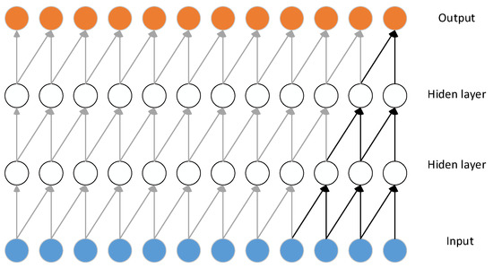
Figure 1.
Schematic diagram of causal convolution.
In Figure 1, each point represents a neuron, and when a sequence signal is input sequentially from left to right, the neurons in the hidden and output layers are only computed using the current or previous sequence signal. Causal convolution extracts features only from the preceding vibration information and is used to provide real-time diagnosis, which allows the trained model to find fault features and make diagnosis faster. However, causal convolution leads to a smaller field of view of the network, and the network must be deepened if valid information is to be extracted from particular preceding signals. These shortcomings will be resolved in other structures.
2.1.2. Dilated Convolution
The dilation factor is introduced in dilated convolution. The dilated convolutional layers are not fully connected when linking neurons from the previous layer; only one out of every few upper layer neurons link to the next layer of neurons. For the input sequence , if the convolution kernel is , the output of the causal convolution is represented by Equation (2):
where is the dilation factor. Figure 2 shows the schematic diagram of dilated convolution.
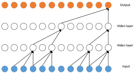
Figure 2.
The schematic diagram of dilated convolution.
As shown in Figure 2, the output of the inflated convolutional layer is intermittently linked to the upper layer neurons by a dilation factor. Unlike the small field of view of the traditional convolution kernel, the dilation factor makes the convolution field of view much larger. It is worth mentioning that, when , this convolutional layer is the traditional convolutional layer. When takes a larger value, the field of view of the convolution layer is larger but more information is lost. In general, a larger value of should not be taken at the lower convolutional layers to prevent the loss of valid information.
2.1.3. Residual Connection
Residual connections are used in ResNet, as proposed by Kaiming He et al. in 2015 [28]. So far, many researchers have demonstrated the need for their ability to prevent overfitting in deep networks. In TCN, the depth of the network increases with the introduction of causal and dilated convolution, which may lead to gradient disappearance or gradient explosion and degradation of the network performance. To solve this problem, residual connections are applied in the network. The input of the model is weighted and fused into the output of the model to obtain the final output :
where is the activation function.
2.2. Attention
When a fault occurs in a motor during operation, the fault source and other mechanical parts collide to produce high-frequency resonance attenuation vibration, which makes the vibration of different signal segments and locations not exactly the same value for fault diagnosis; some features can be used for accurate diagnosis of fault information, and some features have greater interference with the accuracy of fault diagnosis. To measure the importance of these features, attention is used to obtain the weight coefficients of different features.
The attention mechanism [29] was proposed by Bengio’s team in 2014 and has been widely applied in various areas of deep learning in recent years. The attention mechanism is excellent in machine translation tasks. Squeeze-and-excitation networks (SENet) [30], proposed in 2018, apply the attention mechanism to CNN. The SE block first performs squeeze on the feature map obtained by convolution to obtain the global features at channel level and then performs excitation on the global features to learn the relationship between each channel and also obtain the weights of different channels and, finally, multiplies the original feature map to get the final features. Essentially, the SE block performs the attention or the gating on the channel dimension. This attention mechanism allows the model to pay more attention to the most informative channel features and suppress unimportant channel features. Another point is that the SE block is generic, which means that it can be embedded into existing network architectures.
As shown in Figure 3, the SE block includes two main operations: squeeze and excitation. Squeeze is the compression of the dimensional feature map into a vector by a global averaging pooling operation along the direction of the feature channels, where the two-dimensional feature map of each channel is squeezed into a channel feature response value with a global perceptual field. The output after squeeze is obtained by Equation (4):
where denotes the two-dimensional matrix of the current channel. denotes the output after squeeze in the channel .
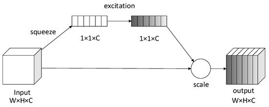
Figure 3.
Schematic of SE block.
Excitation uses two fully connected layers and an activation function to parameterize the gating. The fully connected layer is used to better fuse the full input feature information, while the activation function is used to map the input features to normalized weights between 0 and 1. The output is given by Equation (5):
where is the sigmoid function; is the ReLU activation function; and are the weights of the two fully connected layers; and is the output after the excitation.
Finally, the channel weights output above are weighted to the original features using multiplication, thus, achieving a reassignment of the original features in the channel dimension. The squeeze and excitation modules extract the relevant information through different channels, allowing the model to notice the features of higher relevance.
We introduced squeeze and excitation modules into the TCN. After the original vibration signal was convolved causally, squeeze and excitation were added to the expanded convolution layer, and different vibration features were treated as different channels. Reassigning weights to the nodes of the inflated convolution layer made the network increase its attention to the fault features. The structure of the SE block is shown in Figure 4.
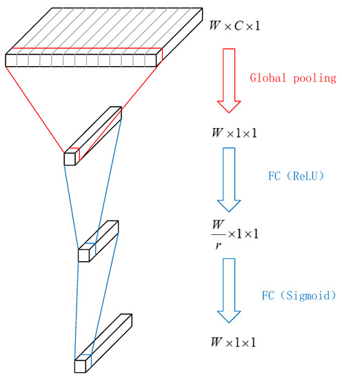
Figure 4.
SE block in TCN.
C is the number of feature maps in each batch; W is the length of the output of a single signal through the dilated convolution layer. By global averaging pooling, this batch was squeezed into a tensor. To reduce the parameters, the size was compressed r in the next layer of the ReLU-activated full convolutional layer. Then, another layer of sigmoid-activated full convolutional layer was passed. The output tensor of size was the attention weight of the input sequence. Finally, each input was scaled with attentional weights to obtain the output of the SE block.
3. Proposed Method
Considering the previous deep learning structures, we propose a TCN model that incorporates an attention mechanism. The whole system structure is shown in Figure 5.
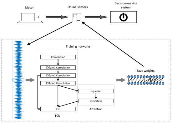
Figure 5.
Motor fault online diagnosis system.
The vibration signal is measured and transmitted by an in-line sensor while the motor is running. The raw vibration signals are fed into a neural network for training and learning fault characteristics. Finally, the trained neural network is used to monitor the operation of the motor online and to diagnose the type of fault in time for the decision-making system to make the right decision when a fault occurs.
As the core part of the system, the network is our proposed TCN that incorporates attention. The input one-dimensional vibration signal sequence is first extracted with features by a conventional convolutional layer. Then, an expanded convolutional layer is used to expand the field of view and down sample. Next, the attention weights of the expanded convolutional layer are changed by SE block and linked to the following expanded convolutional layer by residuals. Finally, an output value is obtained by the full convolution layer to determine what state the motor is running in at the current time. It is worth noting that, in order to obtain the current motor operation as soon as possible, all the convolutional layers in the network are causally convolved to ensure that only the previous vibration signal is used to determine the fault condition.
The TCN has fewer parameters compared to regular convolutional networks and is able to extract features from shorter signals. Additionally, the attention weights obtained by the SE block allow the network to pay attention to useful information in the feature map. The SE block’s addition tends to give the network higher accuracy.
4. Experiments and Discussion
4.1. Machinery Fault Database
This database is composed of 1951 multivariate time series acquired by sensors on a Spectra Quest’s Machinery Fault Simulator (MFS) Alignment-Balance-Vibration (ABVT) at http://www02.smt.ufrj.br/~offshore/mfs/ (Data updated on Wednsday, 16 June 2021). Motor parameters are as follows: frequency range, 700–3600 rpm; system weight, 22 kg; axis diameter, 16 mm; axis length, 520 mm; rotor, 15.24 cm; bearings distance, 390 mm; number of balls, 8; ball diameter, 0.7145 cm; cage diameter, 2.8519 cm. The 1951 comprises six different simulated states: normal function, imbalance fault, horizontal and vertical misalignment faults and inner and outer bearing faults. Each sequence was generated at a 50 kHz sampling rate during 5 s, totaling 250,000 samples. These sequences were measured at different loads and speeds, and the fault settings are described in detail below:
- Normal sequences: there were 49 sequences without any fault, each with a fixed rotation speed within the range of 737 rpm to 3686 rpm with steps of approximately 60 rpm;
- Imbalance faults: there were 333 sequences with load values within the range of 6 g to 35 g. There were roughly 49 sequences in each load value;
- Horizontal parallel misalignment: There were 197 sequences obtained by shifting the motor shaft horizontally by 0.5 mm, 1.0 mm, 1.5 mm and 2.0 mm;
- Vertical parallel misalignment: there were 301 sequences obtained by shifting the motor shaft horizontally by 0.51 mm, 0.63 mm, 1.27 mm, 1.40 mm, 17.8 mm and 1.90 mm;
- Underhang bearing faults: the dataset mounted the three faulty bearings (outer track, rolling elements and inner track) between the rotor and the motor (overhanging position). Because bearing failure is practically undetectable when there is no imbalance, three masses of 6 g, 20 g and 35 g were added to induce a detectable effect, with different rotation frequencies, as before. There were roughly 185 sequences in each type of failure;
- Overhang bearing faults: the same faulty bearing as above was mounted between the rotor and the motor (underhang position). There were roughly 188 sequences in each type of failure.
To test the various performances of the network, we obtained new datasets by filtering the information of the above vibration sequences. We obtained four datasets and the data are shown in the Table 1.

Table 1.
The processed 4 datasets with fault type and number of sequences.
Dataset A had the most comprehensive classification of fault types and locations with 18 categories. Dataset B differed only in fault type, with six categories. Dataset C was filtered to find the most distinctive type of fault characteristic in each fault type. Since each sequence of the raw data was generated at a sampling rate of 50 kHz, we wished to study the fault feature extraction with lower sampling frequency. We obtained the dataset D by undersampling the sequence of 50 kHz to 10 kHz.
4.2. Experiment #1: Network Diagnostic Accuracy
We divided the dataset into a training set and a test set, and they were inputted into the proposed network trained in the first experiment. Due to the large variation in the number of samples for each label in the dataset, in order to avoid the problems caused by unbalanced data, we chose to randomly undersample the data to ensure the same number of samples for each epoch. In addition, each vibration sequence sample contained 250,000 data (the sample of sequences in dataset D contained 5000 data). Obviously, this sequence was too long to be entered by the network in its entirety. Therefore, we set a parameter to let the neural network randomly extract a continuous sequence of length from the pair each time a sample was input. The motor speed was 700 rpm to 3800 rpm when taking the dataset. The value of should contain at least one revolution of the vibration signal of the motor; so, was taken as 150.
We trained the four datasets in TCN, Attention–TCN and 1DCNN several times. The average accuracy of the network on the test sets is shown in Figure 6.
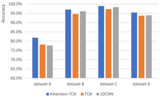
Figure 6.
The average accuracy of the three networks on the four datasets.
From the figure, we can see that the proposed Attention–TCN had higher accuracy compared to the other two on the four datasets. The accuracy of TCN was higher than CNN on dataset A, but, on datasets B and C, the accuracy of TCN was lower than CNN. This was expected because, in datasets B and C, the faults differed significantly, and the CNN was able to extract enough fault features and identify them.
It is also interesting to note that there was a large variance in the accuracy of the network when training dataset D. The accuracy of a single test even differed from the average by 5.2%. We believe that this phenomenon was caused by data loss when undersampling some vibration sequence samples. Therefore, we do not analyze the incorrect diagnosis of dataset D for the remainder of this experiment.
To further investigate the error diagnosis of the network, we plotted the confusion matrix of the network when testing datasets A, B and C, as shown in Figure 7.
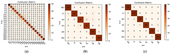
Figure 7.
The confusion matrix of the network: (a) the diagnostic results of dataset A in Attention–TCN; (b) the diagnostic results of dataset B in Attention–TCN; (c) the diagnostic results of dataset C in Attention–TCN.
The ‘IF’ in the figure is equal to the ‘imbalance fault’. ‘NO’ is equal to the ‘normal’. ‘HP’ is equal to the ‘horizontal parallel misalignment’. ‘VP’ is equal to the ‘vertical parallel misalignment’. ‘UB’ is equal to the ‘underhang bearing faults’. ’OB’ is equal to the ‘overhang bearing faults’. Each test sample was a randomly extracted vibration sequence from an untrained sequence.
In the confusion matrix, we found that the faultless samples could be judged correctly. The proposed network could correctly diagnose the type of fault. However, it could not diagnose the specific fault occurrence location well. In the test results of dataset A, the misjudged fault diagnosis essentially made the correct determination of the fault type. Additionally, from the diagnosis results, the bearing failure was more easily misdiagnosed. This is because, with a balanced mass, the signal of a bearing failure was difficult for the sensors mounted on the motor to pick up. In dataset C, we kept only the vibration sequences of bearing failures at the highest weighting. Therefore, the correct bearing fault diagnosis was made in dataset C.
Table 2 shows the accuracy of other deep learning models for motor fault diagnosis.
Table 2.
Comparison of deep learning model in motor fault diagnosis.
The accuracy of the proposed model surpassed the past work of a subset of researchers. The model in this paper was not the best compared with other excellent models. However, longer samples were used in the diagnostic process in others. For example, TFD-DCNN (multi-signal) used multiple signals, and the length of a single sample sequence was 1024. The sample length of Attention–TCN was only 150 to achieve such accuracy. This is of great significance in the task of real-time diagnosis of motor faults.
4.3. Experiment #2: Fault Diagnosis of Short-Sequence Vibration Signals
In addition to having diagnostic accuracy, we wanted the system to be able to alert us more quickly when a motor runs into trouble. So, we studied a trained network to get the correct diagnosis through the shortest possible vibration signal.
In this experiment, we observed the accuracy performance of different networks in the test set by changing the value of length of a single sample sequence for the input network . We set and then input datasets A and B into the three networks to train and test them several times. The experimental results are shown in Figure 8.
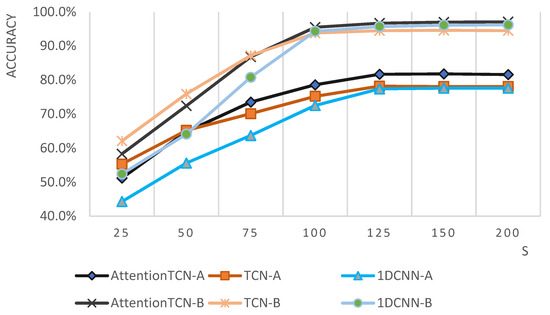
Figure 8.
The test accuracy of the network for different s values.
We found that, when the length of a single vibration signal sample sequence was short, it led to difficulty in extracting fault features for certain sequences. Only when the length of the sample sequence was greater than 125 could we ensure that the fault features of the original vibration signal could be extracted completely. When the length of the vibration sequence was below 75, the entire network performance degraded rapidly. However, the feature extraction ability of TCN was higher compared to CNN in the case of low sequence length. Although Attention–TCN worked better than CNN for all sequence lengths, it had lower accuracy than TCN at low sequence lengths. This also shows that, for vibration sensors of motor operation, TCN needed fewer vibration signals to make a fault diagnosis. This is significant for the real-time failure diagnosis of the motor.
4.4. Experiment #3: Real-Time Motor Fault Diagnosis System
The datasets used in the previous simulation tests were set in a strict environment which does not match the actual operating environment of the motor. Therefore, we hoped to experimentally verify the performance of the proposed network in a real motor real-time diagnosis system. Figure 9 shows the motor platform built.
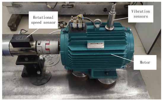
Figure 9.
Failure diagnosis experiment platform.
We used a special motor for the test, and the vibration sensor was mounted on top of the motor housing to collect the vibration signal in the radial direction of the motor. The vibration sensor had an acquisition frequency of 10 kHz and was connected to the computer through a microcontroller. The coupling was equipped with a speed sensor to know the real-time speed of the motor. We set two kinds of fault on the motor: imbalance faults and bearing faults. We saved and stored the trained neural network and its weights in the computer. The vibration sensor acquisition data were sent to the computer via microcontroller communication, and we set the sequence length . Whenever the computer accepted a vibration sequence of length , the sequence was fed into a neural network to calculate and obtain a diagnosis.
We used this platform to collect and store experimental data for the fine-tuning or training of the network model. We kept the speed at 1000/2000/3000 rpm under the same load and collected data when the speed was stable. The duration of each sequence was 10 s, and the acquisition frequency was 10 kHz. One sequence was obtained for each speed for each fault type. The data from the experimental platform were organized into dataset E. The type and data number of each sequence in dataset E are shown in the Table 3.
Table 3.
The categories and sequence length of the dataset E.
We used dataset D to pre-train the neural network and then freeze the previous layers. The last layer, the fully connected layer, was fine-tuned with the dataset E. We set for the test experiment, and the experimental results are shown in Figure 10.
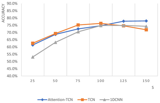
Figure 10.
Accuracy of three network migration learning tests.
From the results, we can see that the accuracy of the network in this case was abysmal. For any sequence length, the fault diagnosis accuracy did not even exceed 80%, and this was just a three-category dataset. This is obviously not ideal as a neural network model for real-time motor fault diagnosis. Bai [27] pointed out in his paper that TCN has no advantage in migration learning due to its insufficient receptive field. Therefore, we decided to train the neural network only through the dataset E. The results of the experiment are shown in the Figure 11.
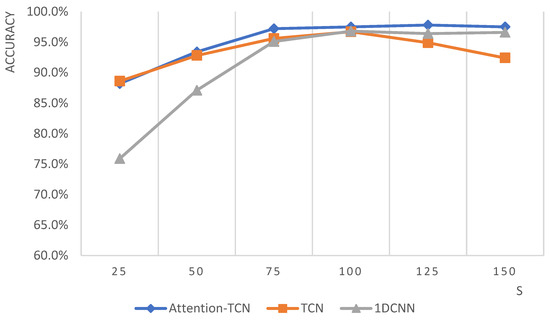
Figure 11.
The accuracy of the three networks in dataset E.
As we expected, the accuracy of the diagnosis became high again when the network abandoned migration learning and was trained entirely by dataset E. The proposed network had higher accuracy than CNN in dealing with short sequences. The Attention–TCN and TCN networks already reached 90% accuracy at sequence lengths of 25–50, yet CNN reached the same diagnostic accuracy only at sequence lengths of 50–75. This indicates that TCN networks are good at extracting features in shorter sequences and are also more suitable for real-time motor fault diagnosis.
In addition, we also found that the accuracy of TCN decreased with the growth of sequence length. This showed the same trend in Experiment #2, but the decline was not significant in Experiment #2. We believe that the feeling field of TCN is still not large enough that it causes information loss when processing more information. The TCN with the introduction of the attention mechanism showed no decrease in accuracy. The presence of the attention mechanism allowed TCN to notice the information that is easily ignored at first when faced with long sequences.
5. Conclusions
We compared the proposed Attention–TCN with TCN and CNN in various datasets, including public datasets and motor experimental platforms. The following conclusions were obtained:
- Attention allows the TCN to be more accurate in motor fault diagnosis tasks and helps the TCN to extract the correct fault features in longer sequences;
- The proposed Attention–TCN can find useful fault information in a shorter vibration sequence and make a correct judgment. This illustrates that Attention–TCN is better than other network models in real-time motor fault diagnosis;
- The migration learning capability of TCN is weak, and even migration under the same fault type can cause a significant decrease in accuracy.
It is worth noting our satisfaction with the excellent performance of the proposed model. However, the real-time fault diagnosis of motors needs to be further studied. Our proposed TCN model, although more suitable than other models, must be used to ensure that the input vibration sequence is of fixed size. Although faster diagnosis is possible with TCN, it is not strictly in “real time”. In our next study, we hope to find a method, such as RNN, which can obtain the correct diagnosis by inputting a signal sequence of arbitrary length. Additionally, we wish to give the model a stronger migration learning capability, which means that all motors, or at least the same types of motor, can use the system directly, instead of having to go through the time-consuming and laborious task of setting up faults and training the model.
Author Contributions
Conceptualization, H.Z., B.G. and B.H.; Methodology, H.Z.; Software, B.H.; Validation, H.Z. and B.G.; Writing—original draft preparation, H.Z. and B.H.; Writing—review and editing, B.G.; Visualization, B.H. and H.Z.; Funding acquisition, B.G. All authors have read and agreed to the published version of the manuscript.
Funding
This research was funded by the project of the National Natural Science Foundation of China under grant 51777048 and the project supported by the Scientific Research Foundation of the Education Department of Heilongjiang Province under grant 135509403.
Institutional Review Board Statement
Not applicable.
Informed Consent Statement
Not applicable.
Data Availability Statement
The data presented in this study are available upon request from the corresponding author. The data are not publicly available due to copyright issues.
Acknowledgments
Thanks for the support of School of Electrical and Electronic Engineering, Harbin University of Science and Technology and College of Computer and Control Engineering, Qiqihar University, in the research process.
Conflicts of Interest
The authors declare no conflict of interest.
References
- Romero-Troncoso, R.J. Multirate Signal Processing to Improve FFT-based Analysis for Detecting Faults in Induction Motors. IEEE Trans. Ind. Inform. 2017, 13, 1291–1300. [Google Scholar] [CrossRef]
- Sapena-Bañó, A.; Pineda-Sanchez, M.; Puche-Panadero, R.; Martinez-Roman, J.; Matic, D. Fault Diagnosis of Rotating Electrical Machines in Transient Regime Using a Single Stator Current’s FFT. IEEE Trans. Instrum. Meas. 2015, 64, 3137–3146. [Google Scholar] [CrossRef] [Green Version]
- Antonino-Daviu, J.A.; Riera-Guasp, M.; Pons-Llinares, J.; Roger-Folch, J.; P´erez, R.B.; Charlton-P´erez, C. Toward Condition Monitoring of Damper Windings in Synchronous Motors via EMD Analysis. IEEE Trans. Energy Convers. 2012, 27, 432–439. [Google Scholar] [CrossRef]
- Valles-Novo, R.; Jesus Rangel-Magdaleno, J.J.; Ramirez-Cortes, J.M.; Peregrina-Barreto, H.; Morales-Caporal, R. Empirical Mode Decomposition Analysis for Broken-Bar Detection on Squirrel Cage Induction Motors. IEEE Trans. Instrum. Meas. 2015, 64, 1118–1128. [Google Scholar] [CrossRef]
- Heydarzadeh, M.; Zafarani, M.; Nourani, M.; Akin, B. A Wavelet-Based Fault Diagnosis Approach for Permanent Magnet Synchronous Motors. IEEE Trans. Energy Convers. 2019, 34, 761–772. [Google Scholar] [CrossRef]
- Sangeetha, P.; Hemamalini, S. Rational-Dilation Wavelet Transform Based Torque Estimation from Acoustic Signals for Fault Diagnosis in a Three Phase Induction Motor. IEEE Trans. Ind. Inform. 2019, 15, 3492–3501. [Google Scholar] [CrossRef]
- Jiang, X.X.; Shen, C.Q.; Shi, J.J.; Zhu, Z.K. Initial center frequency-guided VMD for fault diagnosis of rotating machines. J. Sound Vib. 2018, 435, 36–55. [Google Scholar] [CrossRef]
- Wang, Y.Y.; Wei, Z.X.; Yang, J.W. Feature Trend Extraction and Adaptive Density Peaks Search for Intelligent Fault Diagnosis of Machines. IEEE Trans. Ind. Inform. 2019, 15, 105–115. [Google Scholar] [CrossRef]
- Fu, Q.; Jing, B.; He, P.J.; Si, S.H.; Wang, Y. Fault Feature Selection and Diagnosis of Rolling Bearings Based on EEMD and Optimized Elman-AdaBoost Algorithm. IEEE Sens. J. 2018, 18, 5024–5034. [Google Scholar] [CrossRef]
- Kankar, P.K.; Sharma, S.C.; Harsha, S.P. Fault diagnosis of ball bearings using machine learning methods. Expert Syst. Appl. 2011, 38, 1876–1886. [Google Scholar] [CrossRef]
- Praveenkumar, T.; Saimurugan, M.; Krishnakumar, P.; Ramachandran, K.I. Fault diagnosis of automobile gearbox based on machine learning techniques. Procedia Eng. 2014, 97, 2092–2098. [Google Scholar] [CrossRef] [Green Version]
- Samanta, B.; Nataraj, C. Use of particle swarm optimization for machinery fault detection. Eng. Appl. Artif. Intell. 2009, 22, 308–316. [Google Scholar] [CrossRef]
- Samanta, B.; Al-Balushi, K.R.; Al-Araimi, S.A. Artificial neural networks and genetic algorithm for bearing fault detection. Soft. Comput. 2006, 10, 264–271. [Google Scholar] [CrossRef]
- Hinton, G.E.; Salakhutdinov, R.R. Reducing the Dimensionality of Data with Neural Networks. Science 2006, 313, 504–507. [Google Scholar] [CrossRef] [Green Version]
- Sun, J.D.; Yan, C.H.; Wen, J.T. Intelligent bearing fault diagnosis method combining compressed data acquisition and deep learning. IEEE Trans. Instrum. Meas. 2018, 67, 185–195. [Google Scholar] [CrossRef]
- Jiang, G.Q.; He, H.B.; Xie, P.; Tang, Y.F. Stacked multilevel-denoising autoencoders: A new representation learning approach for wind turbine gearbox fault diagnosis. IEEE Trans. Instrum. Meas. 2017, 66, 2391–2402. [Google Scholar] [CrossRef]
- Ma, M.; Sun, C.; Chen, X.F. Discriminative deep belief networks with ant colony optimization for health status assessment of machine. IEEE Trans. Instrum. Meas. 2017, 66, 3115–3125. [Google Scholar] [CrossRef]
- Palacios, R.H.C.; Silva, I.N.; Goedtel, A.; Godoy, W.F. Diagnosis of stator faults severity in induction motors using two intelligent approaches. IEEE Trans. Ind. Inform. 2017, 13, 1681–1691. [Google Scholar] [CrossRef]
- Ding, X.X.; He, Q.B. Energy-Fluctuated Multiscale Feature Learning With Deep ConvNet for Intelligent Spindle Bearing Fault Diagnosis. IEEE Trans. Instrum. Meas. 2017, 66, 1926–1935. [Google Scholar] [CrossRef]
- Liang, P.F.; Deng, C.; Wu, J.; Yang, Z.X. Intelligent fault diagnosis of rotating machinery via wavelet transform, generative adversarial nets and convolutional neural network. Measurement 2020, 159, 107768. [Google Scholar] [CrossRef]
- Shao, S.Y.; McAleer, S.; Yan, R.Q.; Baldi, P. Highly Accurate Machine Fault Diagnosis Using Deep Transfer Learning. IEEE Trans. Ind. Inform. 2019, 15, 2446–2455. [Google Scholar] [CrossRef]
- Ince, T.; Kiranyaz, S.; Eren, L. Real-Time Motor Fault Detection by 1-D Convolutional Neural Networks. IEEE Trans. Ind. Electron. 2016, 63, 7067–7075. [Google Scholar] [CrossRef]
- Zhang, W.; Peng, G.L.; Li, C.H.; Chen, Y.H.; Zhang, Z.J. A New Deep Learning Model for Fault Diagnosis with Good Anti-Noise and Domain Adaptation Ability on Raw Vibration Signals. Sensors 2017, 17, 425. [Google Scholar] [CrossRef] [PubMed]
- Lin, S.L. Application Combining VMD and ResNet101 in Intelligent Diagnosis of Motor Faults. Sensors 2021, 21, 6065. [Google Scholar] [CrossRef] [PubMed]
- Long, Z.; Zhang, X.F.; He, M.; Huang, S.D.; Qin, G.J.; Song, D.Y.; Tang, Y.; Wu, G.P.; Liang, W.Z.; Shao, H.D. Motor Fault Diagnosis Based on Scale Invariant Image Features. IEEE Trans. Ind. Inform. 2021, 18, 1605–1617. [Google Scholar] [CrossRef]
- Shao, S.Y.; Yan, R.Q.; Lu, Y.D.; Wang, P.; Gao, R. DCNN-based Multi-signal Induction Motor Fault Diagnosis. IEEE Trans. Instrum. Meas. 2020, 69, 2658–2669. [Google Scholar] [CrossRef]
- Lea, C.; Vidal, R.; Reiter, A.; Hager, G.D. Temporal convolutional networks: A unified approach to action segmentation. In Proceedings of the 14th European Conference on Computer Vision, Amsterdam, The Netherlands, 11–14 October 2016. [Google Scholar]
- He, K.M.; Zhang, X.Y.; Ren, S.P.; Sun, J. Deep Residual Learning for Image Recognition. In Proceedings of the IEEE Computer Society Conference on Computer Vision and Pattern Recognition (CVPR 2016), Las Vegas, NV, USA, 26 June–1 July 2016. [Google Scholar]
- Bahdanau, D.; Cho, K.; Bengio, Y. Neural machine translation by jointly learning to align and translate. In Proceedings of the 3rd International Conference on Learning Representations, San Diego, CA, USA, 7–9 May 2015. [Google Scholar]
- Hu, J.; Shen, L.; Albanie, S.; Sun, G.; Wu, E.H. Squeeze-and-excitation networks. IEEE Trans. Pattern Anal. Mach. Intell. 2020, 42, 2011–2023. [Google Scholar] [CrossRef] [Green Version]
- Sun, W.J.; Zhao, R.; Yan, R.Q.; Shao, S.Y.; Chen, X.F. Convolutional Discriminative Feature Learning for Induction Motor Fault Diagnosis. IEEE Trans. Ind. Inform. 2017, 13, 1350–1359. [Google Scholar] [CrossRef]
- Sun, W.J.; Shao, S.Y.; Zhao, R.; Yan, R.Q.; Zhang, X.W.; Chen, X.F. A sparse auto-encoder-based deep neural network approach for induction motor faults classification. Measurement 2016, 89, 171–178. [Google Scholar] [CrossRef]
- Shao, S.Y.; Sun, W.J.; Yan, R.Q.; Wang, P.; Gao, R.X. A deep learning approach for fault diagnosis of induction motors in manufacturing. CJME (Engl. Ed.) Chin. J. Mech. Eng. 2017, 30, 1347–1356. [Google Scholar] [CrossRef] [Green Version]
Publisher’s Note: MDPI stays neutral with regard to jurisdictional claims in published maps and institutional affiliations. |
© 2022 by the authors. Licensee MDPI, Basel, Switzerland. This article is an open access article distributed under the terms and conditions of the Creative Commons Attribution (CC BY) license (https://creativecommons.org/licenses/by/4.0/).