
Investigation of the Aerodynamic Performance of the Miller Cycle from Transparent Engine Experiments and CFD Simulations

 , ,
, ,  ,
,
Abstract
:1. Introduction
2. Experimental Setup
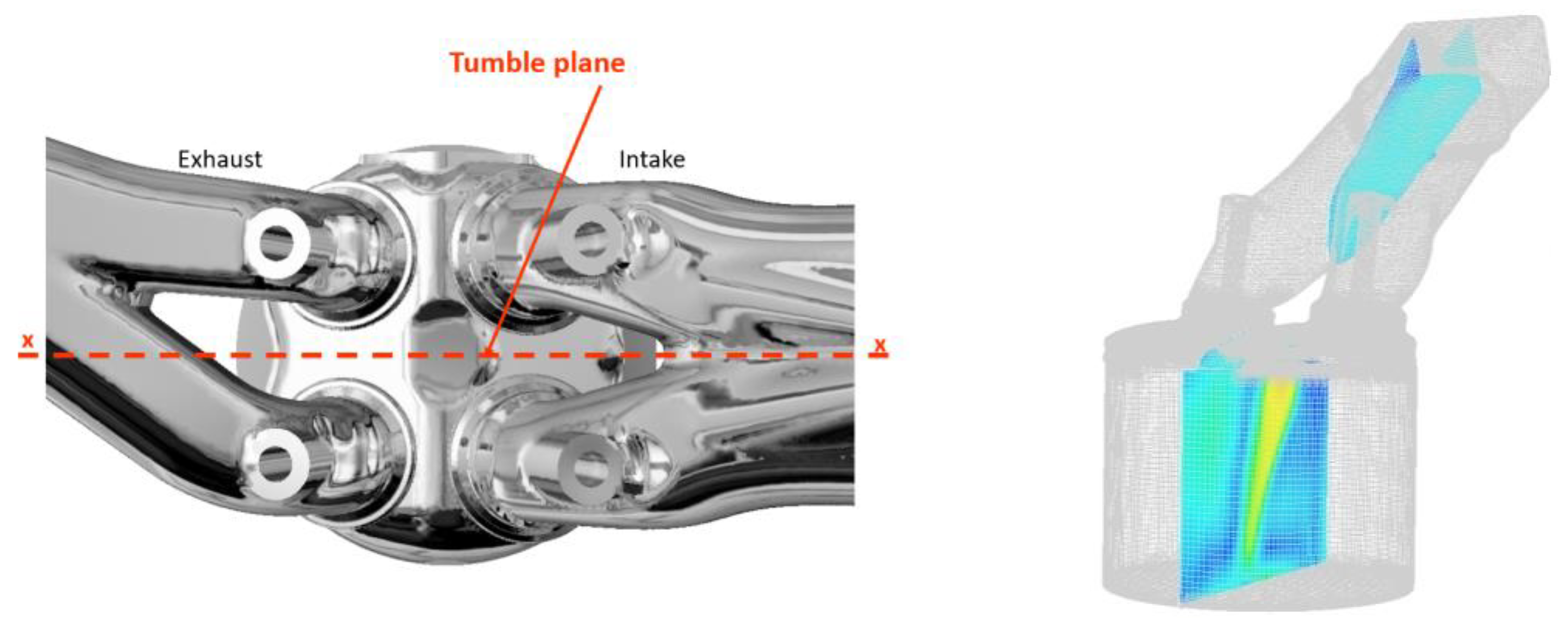
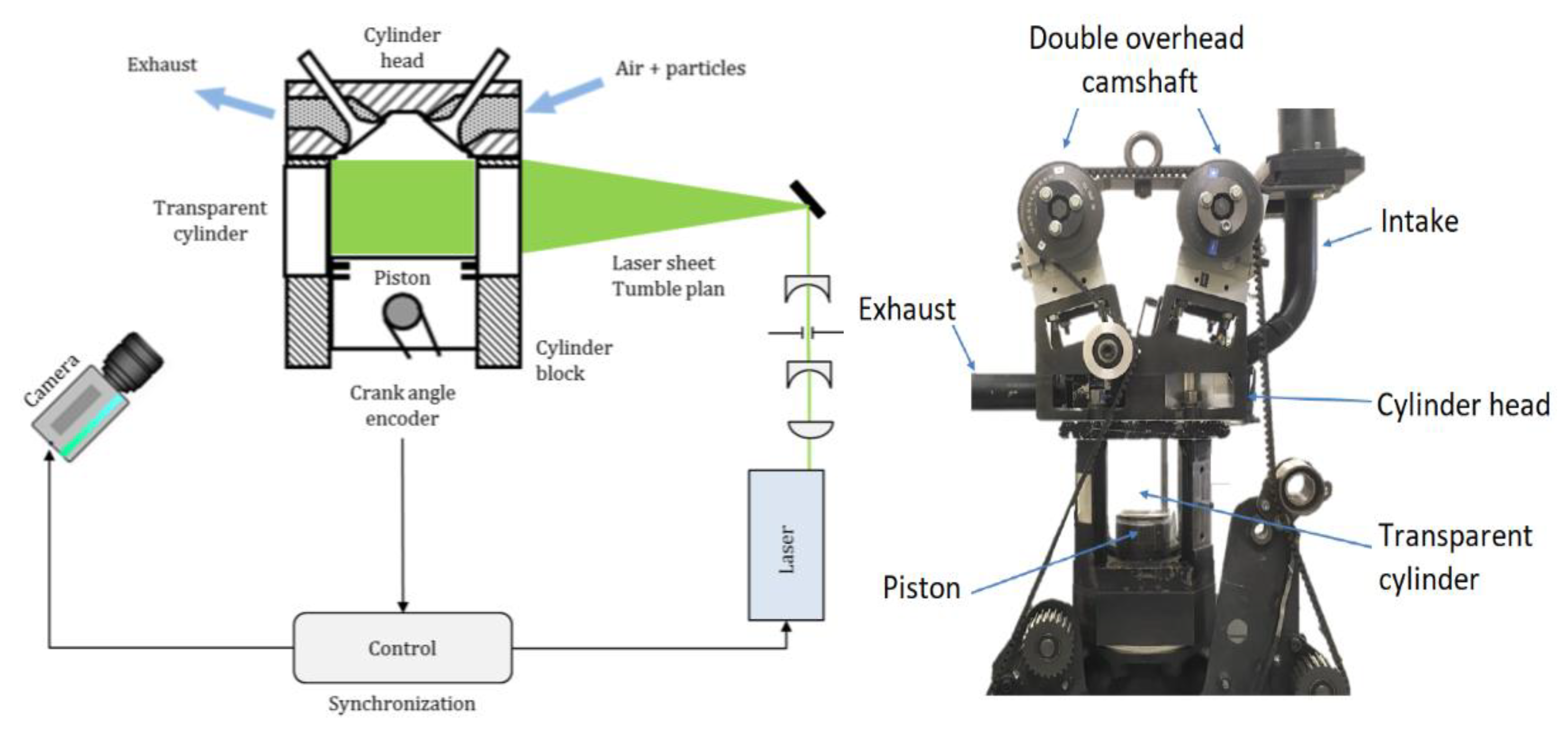
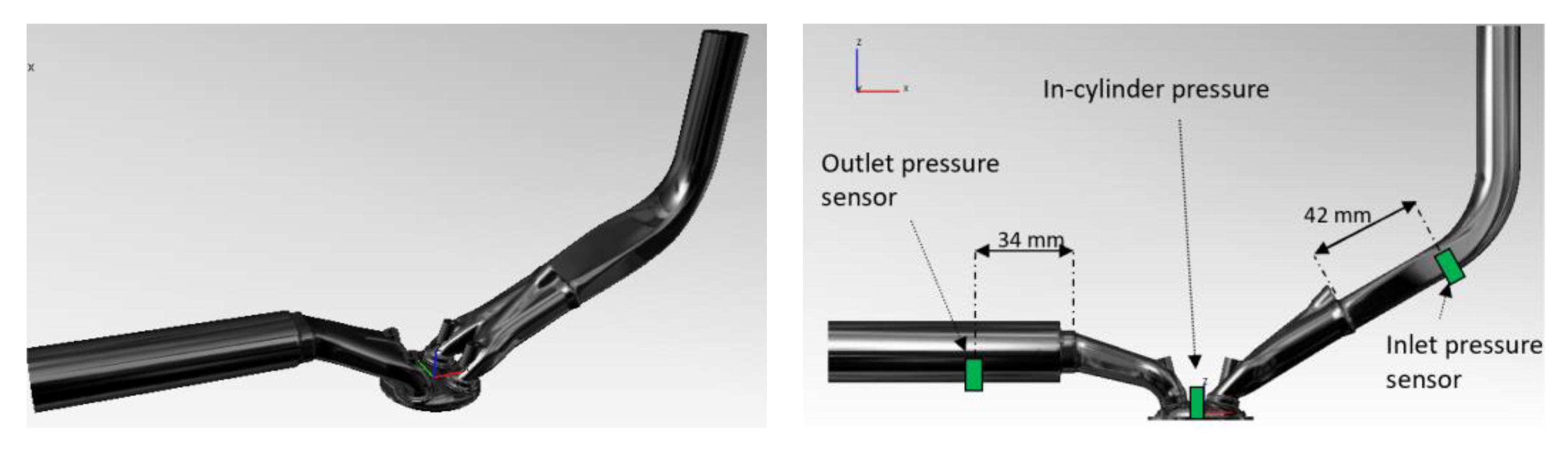
2.1. Model Engine
2.2. Particle Image Velocimetry Measurements
3. Numerical Investigations
3.1. Reynolod-Average Navier–Stokes Formalism and Turbulence Model
3.2. Simulation Description
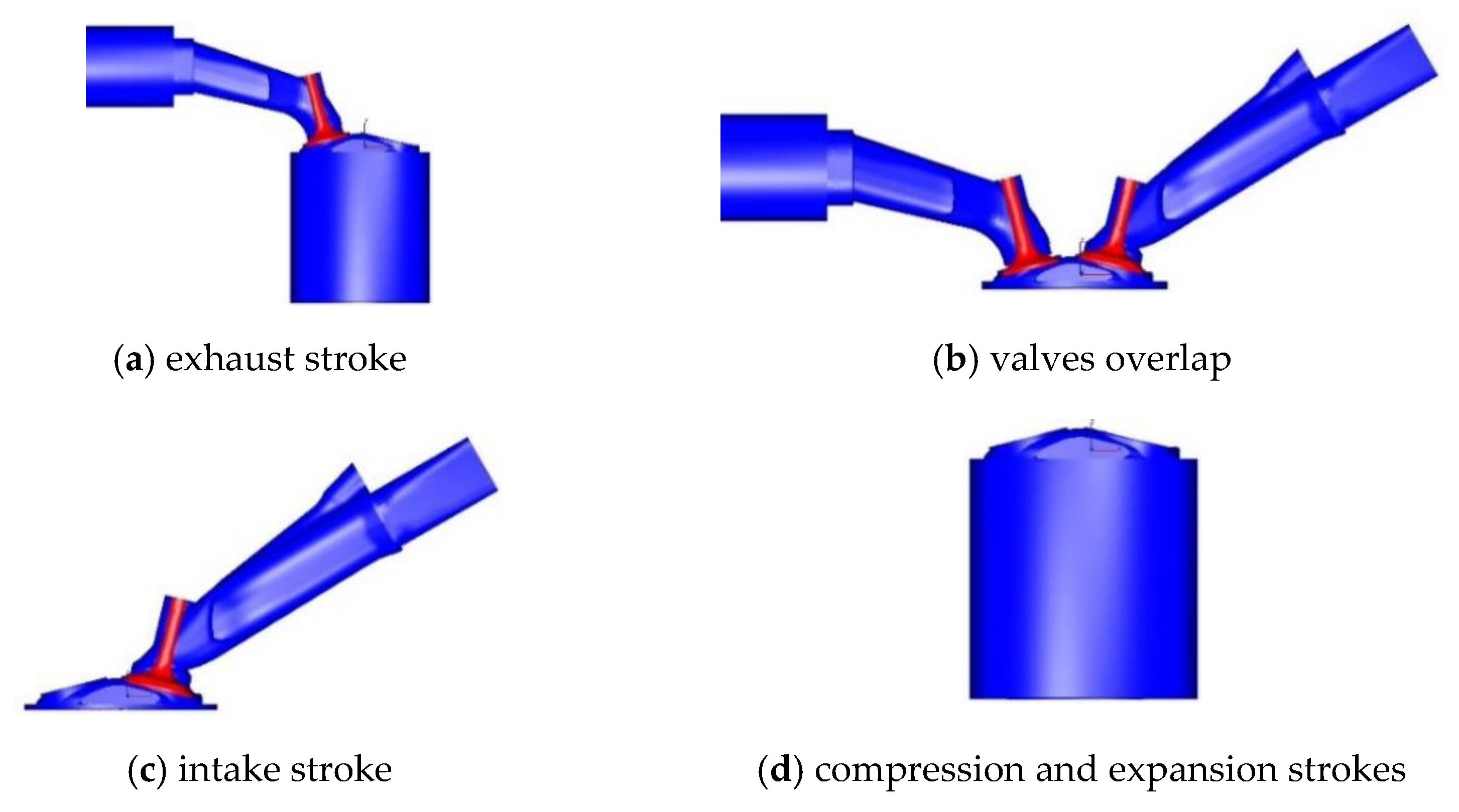
- the exhaust duct, the exhaust ports, and the cylinder → exhaust stroke (Figure 7a);
- the exhaust, the cylinder, and the intake → valves overlap (Figure 7b);
- the intake duct, the intake ports, and the cylinder → intake stroke (Figure 7c);
- the cylinder → compression and power/expansion stroke (Figure 7d).
4. Results
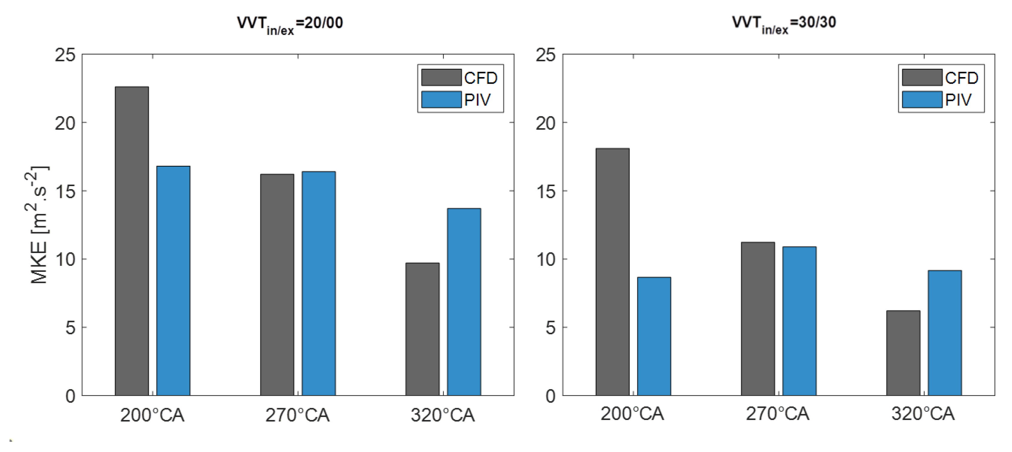
4.1. Mean Flow
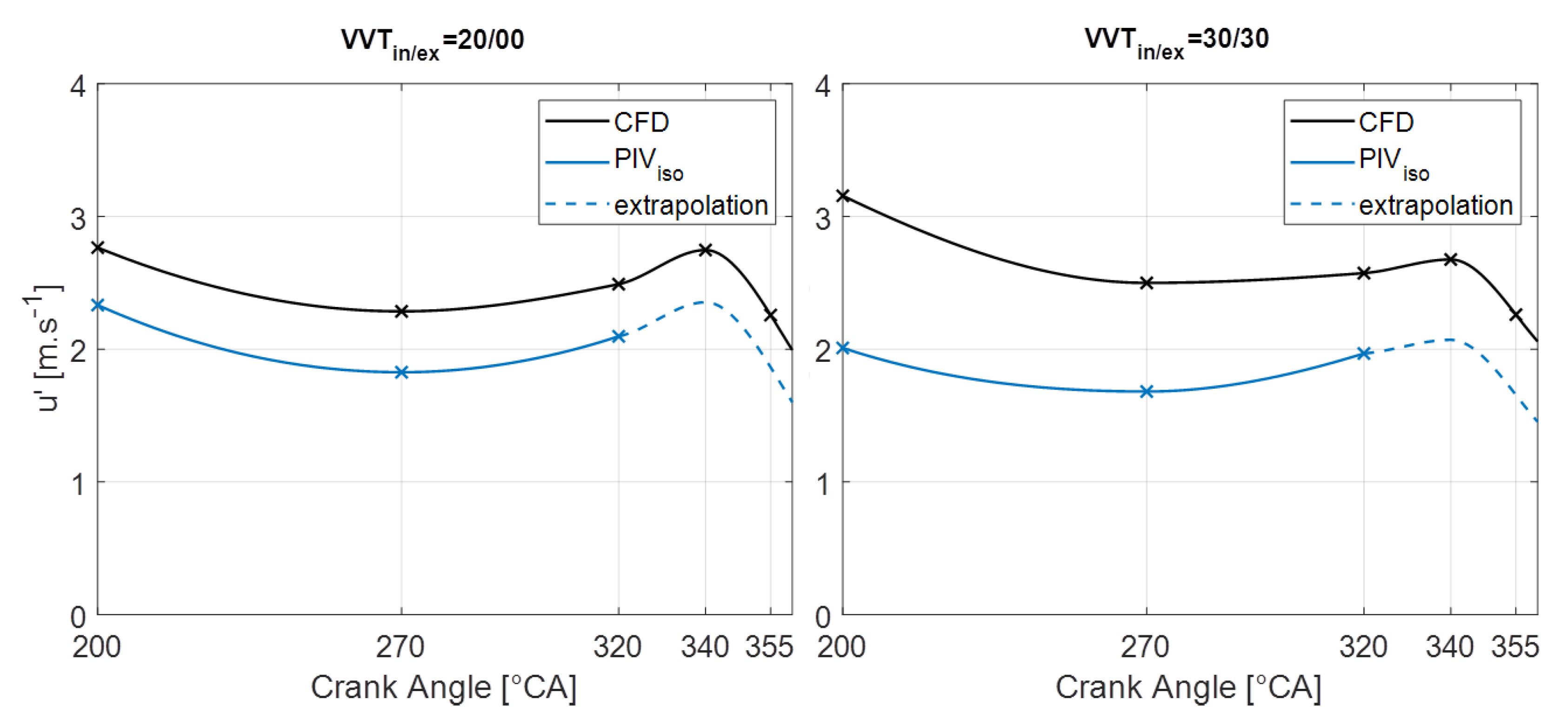
4.2. Turbulent Flow
5. Conclusions and Future Works
Author Contributions
Funding
Informed Consent Statement
Data Availability Statement
Acknowledgments
Conflicts of Interest
Acronyms and Notations
| 0D | zero dimensional |
| 3D | three dimensional |
| BC | boundary condition |
| BDC | bottom dead center |
| CA | crank angle |
| CFD | computational fluid dynamics |
| CPU | central processing unit |
| CO2 | carbon dioxide |
| EIVC | early intake valve closing |
| GB | gigabyte |
| GHz | gigahertz |
| IC | internal combustion |
| in/ex | intake/exhaust |
| LES | large eddy simulation |
| LIVC | late intake valve closing |
| MKE, K [m2·s−2] | mean kinetic energy |
| NOx | nitrogen oxides |
| PIV | particle image velocimetry |
| RAM | random access memory |
| RANS | Reynolds-averaged Navier–Stokes |
| RDE | real driving emissions |
| rpm | revolutions per minute |
| RSM | Reynolds stress model |
| SI | spark ignition |
| TDC | top dead center |
| TKE, K [m2·s−2] | turbulent kinetic energy |
| URANS | unsteady Reynolds-averaged Navier–Stokes |
| VGT | variable geometry turbine |
| VVT | variable valve timing |
| Abb [m2] | leakage section/area |
| blow-by mass flow rate | |
| Pcyl [Pa] | in-cylinder pressure |
| Patm [Pa] | atmospheric pressure |
| Dcyl [m] | bore |
| gap [m] | leakage gap |
| max. number of the grid’s nodes | |
| X flow velocity at the k node | |
| Y flow velocity at the k node | |
| velocity fluctuation of the i component | |
| velocity of the i component | |
| mean velocity of the i component | |
| mean TKE per mass unity for the CFD/PIV case | |
| ζ | eddy viscosity |
| ε | rate of dissipation |
| ω | specific rate of dissipation |
| f | relaxation function |
| v2 | velocity scale |
| g | the square root of a characteristic turbulent time scale |
References
- Miller, R. Miller cycle. Engine. U.S. Patent 2817322, 24 December 1957. [Google Scholar]
- Mo, H.; Huang, Y.; Mao, X.; Zhuo, B. Investigations on the Potential of Miller Cycle for Performance Improvement of Gas Engine. Glob. J. Res. Eng. B Automot. Eng. 2016, 16, 36–46. [Google Scholar]
- Braun, M.; Klaas, M.; Schröder, W. Influence of Miller Cycles on Engine Air Flow. SAE Int. J. Engines 2018, 11, 161–178. [Google Scholar] [CrossRef]
- Huang, Z.-M.; Shen, K.; Wang, L.; Chen, W.-G.; Pan, J.-Y. Experimental study on the effects of the Miller cycle on the performance and emissions of a downsized turbocharged gasoline direct injection engine. Adv. Mech. Eng. 2020, 12, 1–9. [Google Scholar] [CrossRef]
- Wang, Y.; Lin, L.; Zeng, S.; Huang, J.; Roskilly, A.P.; He, Y.; Huang, X.; Li, S. Application of the Miller cycle to reduce NOx emissions from petrol engines. Appl. Energy 2008, 85, 463–474. [Google Scholar] [CrossRef]
- Transport & Environment. Road to Zero: The Last EU Emission Standard for Cars, Vans, Buses and Trucks. 2020. Available online: https://www.transportenvironment.org/wp-content/uploads/2021/06/2020_04_Road_to_Zero_last_EU_emission_standard_cars_vans_buses_trucks.pdf (accessed on 16 March 2022).
- Budack, R.; Wurms, R.; Mendl, G.; Heiduk, T. The New Audi 2.0-l I4 TFSI Engine. MTZ Worldw. 2016, 77, 16–23. [Google Scholar] [CrossRef]
- Demmelbauer-Ebner, W.; Persigehl, K.; Görke, M.; Werstat, E. The New 1.5-l Four-cylinder TSI Engine from Volkswagen. MTZ Worldw. 2017, 78, 16–23. [Google Scholar] [CrossRef]
- Demmelbauer-Ebner, W.; Theobald, J.; Worm, J.; Scheller, P. The new 1.5-l EA211 TGI evo. MTZ Worldw. 2018, 79, 16–21. [Google Scholar] [CrossRef]
- European Automobile Manufacturers Association. What Is the Real Driving Emissions (RDE) Test? Car Emissions Testing Facts. 2018. Available online: http://www.caremissionstestingfacts.eu/rde-real-driving-emissions-test/ (accessed on 17 March 2022).
- Nose, H.; Inoue, T.; Katagiri, S.; Sakai, A.; Kawasaki, T.; Okamura, M. Fuel Enrichment Control System by Catalyst Temperature Estimation to Enable Frequent Stoichiometric Operation at High Engine Speed/Load Condition. In Proceedings of the SAE 2013 World Congress & Exhibition, Detroit, MI, USA, 16–18 April 2013; pp. 16–18. [Google Scholar] [CrossRef]
- Morand, N.; Agnew, G.; Bontemps, N.; Jeckel, D. Variable Nozzle Turbine Turbocharger for Gasoline ‘Miller’ Engine. MTZ Worldw. 2016, 78, 40–45. [Google Scholar] [CrossRef]
- Penzel, M.; Bevilacqua, V.; Böger, M. Meeting Future Emission Standards with Turbocharged High-Performance Gasoline Engines. MTZ Worldw. 2020, 81, 16–25. [Google Scholar] [CrossRef]
- Scheidt, I.M.; Brands, I.C.; Kratzsch, M.; Günther, M. Combined Miller/Atkinson Strategy for Future Downsizing Concepts. MTZ Worldw. 2014, 75, 4–11. [Google Scholar] [CrossRef]
- Niculae, M.; Clenci, A.; Iorga-Simăn, V.; Niculescu, R. Évaluation de l’impact du masquage des soupapes d’admission et de l’augmentation de la course du piston sur l’aérodynamique interne du moteur Miller. Entropie Thermodyn. Énergie Environ. Économie 2021, 1. [Google Scholar] [CrossRef]
- Xu, J.; Guo, T.; Feng, Y.; Sun, M. Numerical investigation of Miller cycle with EIVC and LIVC on a high compression ratio gasoline engine. Sci. Prog. 2021, 104, 368504211023640. [Google Scholar] [CrossRef] [PubMed]
- Cao, Y. Sensibilité d’un Ecoulement de Rouleau Compressé et des Variations Cycle à Cycle Associées à des Paramètres de Remplissage Moteur. Ph.D. Thesis, ENSMA, Chasseneuil-du-Poitou, France, 2014. [Google Scholar]
- El-Adawy, M.; Heikal, M.; Aziz, A.R.A.; Opatola, R.A. Stereoscopic particle image velocimetry for engine flow measurements: Principles and applications. Alex. Eng. J. 2021, 60, 3327–3344. [Google Scholar] [CrossRef]
- Matsuda, M.; Yokomori, T.; Shimura, M.; Minamoto, Y.; Tanahashi, M.; Iida, N. Development of cycle-to-cycle variation of the tumble flow motion in a cylinder of a spark ignition internal combustion engine with Miller cycle. Int. J. Engine Res. 2020, 22, 1512–1524. [Google Scholar] [CrossRef]
- EBaum, E.; Peterson, B.; Surmann, C.; Michaelis, D.; Böhm, B.; Dreizler, A. Tomographic PIV measurements in an IC engine. In Proceedings of the 16th International Symposium on Applications of Laser Techniques to Fluid Mechanics Conference, Lisbon, Portugal, 16–19 July 2012; pp. 1–12. [Google Scholar]
- Lee, H. Thermographic PIV for Turbulent Flux Measurement. Technische Universität Darmstadt. 2016. Available online: https://tuprints.ulb.tu-darmstadt.de/5532/ (accessed on 18 March 2022).
- Jahanmiri, M. Particle Image Velocimetry: Fundamentals and Its Applications. Goteborg. 2011. Available online: https://www.academia.edu/2263312/Particle_Image_Velocimetry_Fundamentals_and_Its_Applications (accessed on 18 March 2022).
- Lawson, J.M.; Dawson, J.R. A scanning PIV method for fine-scale turbulence measurements. Exp. Fluids 2014, 55, 1857. [Google Scholar] [CrossRef]
- Adrian, R.J. Measurement Potential of Laser Speckle Velocimetry. NASA Conference Publication. October 1982. Available online: https://www.researchgate.net/publication/4675662_Measurement_potential_of_laser_speckle_velocimetry (accessed on 19 March 2022).
- Koochesfahani, M.M.; Nocera, D.G. Molecular Tagging Velocimetry. In Springer Handbook of Experimental Fluid Mechanics; Tropea, H.C., Yarin, A., Foss, J.F., Eds.; Springer: Berlin/Heidelberg, Germany, 2007. [Google Scholar] [CrossRef]
- Meier, A.H.; Roesgen, T. Imaging laser Doppler velocimetry. Exp. Fluids 2011, 52, 1017–1026. [Google Scholar] [CrossRef]
- Hanjalić, K.; Popovac, M.; Hadžiabdić, M. A robust near-wall elliptic-relaxation eddy-viscosity turbulence model for CFD. Int. J. Heat Fluid Flow 2004, 25, 1047–1051. [Google Scholar] [CrossRef]
- Basara, B. Analysis of the performance of linear and non-linear K-ε-ζ-F turbulence model on various applications. In Proceedings of the Fluids Engineering Division Summer Meeting, Miami, FL, USA, 17–20 July 2006; pp. 239–247. [Google Scholar] [CrossRef]
- Alfonsi, G. Reynolds-Averaged Navier–Stokes Equations for Turbulence Modeling. Appl. Mech. Rev. 2009, 62, 040802. [Google Scholar] [CrossRef]
- Yang, X.; Gupta, S.; Kuo, T.-W.; Gopalakrishnan, V. RANS and large Eddy simulation of internal combustion engine flows—A comparative study. J. Eng. Gas Turbines Power 2014, 136, 051507. [Google Scholar] [CrossRef]
- Hasse, C.; Sohm, V.; Durst, B. Numerical investigation of cyclic variations in gasoline engines using a hybrid URANS/LES modeling approach. Comput. Fluids 2009, 39, 25–48. [Google Scholar] [CrossRef]
- Hasse, C.; Sohm, V.; Durst, B. Detached eddy simulation of cyclic large scale fluctuations in a simplified engine setup. Int. J. Heat Fluid Flow 2009, 30, 32–43. [Google Scholar] [CrossRef]
- SBuhl, S.; Dietzsch, F.; Buhl, C.; Hasse, C. Comparative study of turbulence models for scale-resolving simulations of internal combustion engine flows. Comput. Fluids 2017, 156, 66–80. [Google Scholar] [CrossRef]
- Hemmingsen, C.S.; Ingvorsen, K.M.; Mayer, S.; Walther, J.H. LES And URANS simulations of the swirling flow in a dynamic model of a uniflow-scavenged cylinder. Int. J. Heat Fluid Flow 2016, 62, 213–223. [Google Scholar] [CrossRef]
- Krastev, V.; Di Ilio, G.; Falcucci, G.; Bella, G. Notes on the hybrid URANS/LES turbulence modeling for Internal Combustion Engines simulation. Energy Procedia 2018, 148, 1098–1104. [Google Scholar] [CrossRef]
- Enaux, B.; Granet, V.; Vermorel, O.; Lacour, C.; Thobois, L.; Dugué, V.; Poinsot, T. Large Eddy Simulation of a Motored Single-Cylinder Piston Engine: Numerical Strategies and Validation. Flow Turbul. Combust. 2010, 86, 153–177. [Google Scholar] [CrossRef]
- Bakker, A. Lectures on Applied Computational Fluid Dynamics. Dartmouth College. 2008. Available online: https://www.bakker.org/Lectures-Applied-CFD.pdf (accessed on 15 January 2020).
- Krastev, V.K.; Silvestri, L.; Falcucci, G.; Bella, G. A Zonal-LES Study of Steady and Reciprocating Engine-Like Flows Using a Modified Two-Equation des Turbulence Model. SAE Technical Paper, September 2017. [Google Scholar] [CrossRef]
- Krastev, V.; Silvestri, L.; Bella, G. Effects of Turbulence Modeling and Grid Quality on the Zonal URANS/LES Simulation of Static and Reciprocating Engine-Like Geometries. SAE Int. J. Engines 2018, 11, 669–686. [Google Scholar] [CrossRef]
- Karbon, M.; Sleiti, A.K. Turbulence Modeling Using Z-F Model and RSM for Flow Analysis in Z-SHAPE Ducts. J. Eng. 2020, 2020, 4854837. [Google Scholar] [CrossRef]
- Durbin, P.A. Near-Wall Turbulence Closure Modeling without “Damping Functions”. Theor. Comput. Fluid Dyn. 1991, 3, 1–13. [Google Scholar] [CrossRef]
- Advanced Simulation Technologies. In AVL FIRE—Turbulence Modeling (Brochure); AVL List GmbH: Graz, Austria, 2009.
- Perceau, M.; Guibert, P.; Guilain, S. Zero-dimensional turbulence modeling of a spark ignition engine in a Miller cycle «Dethrottling» approach using a variable valve timing system. Appl. Therm. Eng. 2021, 199, 117535. [Google Scholar] [CrossRef]
- Kirkpatrick, A.T.; Ferguson, C.R. Internal Combustion Engines, 3rd ed.; Wiley: Hoboken, NJ, USA, 2016. [Google Scholar] [CrossRef]


| Max. Cell Size | Max. Number of Cells | Repartition | (%) | Min. Number of Cells | Repartition | (%) |
|---|---|---|---|---|---|---|
| 1 mm | 7,527,028 (@180° CA) | hexahedral | 82 | 2,866,060 (@360° CA) | hexahedral | 81.5 |
| tetrahedral | 0.67 | tetrahedral | 1.01 | |||
| prismatic | 10.5 | prismatic | 13.89 | |||
| pyramidal | 5.92 | pyramidal | 7.9 |
| Max. Cell Size [mm] | 1.3 | 1.0 | 0.7 |
|---|---|---|---|
| Meshing time [hours] | 9 | 17 | 27 |
| Simulation time [hours] | 19 | 96 | 185 |
Publisher’s Note: MDPI stays neutral with regard to jurisdictional claims in published maps and institutional affiliations. |
© 2022 by the authors. Licensee MDPI, Basel, Switzerland. This article is an open access article distributed under the terms and conditions of the Creative Commons Attribution (CC BY) license (https://creativecommons.org/licenses/by/4.0/).
Share and Cite
Perceau, M.; Guibert, P.; Clenci, A.; Iorga-Simăn, V.; Niculae, M.; Guilain, S. Investigation of the Aerodynamic Performance of the Miller Cycle from Transparent Engine Experiments and CFD Simulations. Machines 2022, 10, 467. https://doi.org/10.3390/machines10060467
Perceau M, Guibert P, Clenci A, Iorga-Simăn V, Niculae M, Guilain S. Investigation of the Aerodynamic Performance of the Miller Cycle from Transparent Engine Experiments and CFD Simulations. Machines. 2022; 10(6):467. https://doi.org/10.3390/machines10060467
Chicago/Turabian StylePerceau, Marcellin, Philippe Guibert, Adrian Clenci, Victor Iorga-Simăn, Mihai Niculae, and Stéphane Guilain. 2022. "Investigation of the Aerodynamic Performance of the Miller Cycle from Transparent Engine Experiments and CFD Simulations" Machines 10, no. 6: 467. https://doi.org/10.3390/machines10060467