
An Optimized VMD Method for Predicting Milling Cutter Wear Using Vibration Signal

1
Key Lab. of NC Machine Tools and Integrated Manufacturing Equipment of the Ministry of Education & Key Lab. of Manufacturing Equipment of Shaanxi Province, Xi’an University of Technology, Xi’an 710048, China
2
Shandong Deed Precision Machine Tool Co., Ltd., Jining 272114, China
3
Xi’an Jingdiao Precision Mechanical Engineering Co., Ltd., Xi’an 710119, China
4
Department of Rural Regional Development, College of Humanities and Urban-Rural Development, Beijing University of Agriculture, Beijing 102206, China
*
Author to whom correspondence should be addressed.
Machines 2022, 10(7), 548; https://doi.org/10.3390/machines10070548
Submission received: 27 May 2022
/
Revised: 22 June 2022
/
Accepted: 1 July 2022
/
Published: 6 July 2022
(This article belongs to the Special Issue Noise and Vibration in Machine Tools)
Abstract
:Tool wear has a negative impact on machining quality and efficiency. As for the nonlinear and non-stationary characteristics of vibration signals and strong background noises during the milling process, an identification method of the milling cutter wear state based on the optimized Variational Mode Decomposition (VMD) was proposed, in which the objective function is to minimize the Envelope Entropy (Ep); the various modes of the vibration signal are decomposed using the self-adaptive optimization parameters with Differential Evolution (DE). According to the cross-correlation coefficient in the frequency domain between Intrinsic Mode Function (IMF) and the original signals, the informative IMF components were selected as the sensitive IMF components to superimpose the reconstruction signal and extract the eigenvalues. The mapping relationship between the eigenvalues and the milling cutter wear degree is established by the Naive Bayes classifier method. The experimental results under the various operation conditions indicate that the proposed optimized VMD method possesses an excellent generalization performance. Compared with Empirical Mode Decomposition (EMD) and Ensemble Empirical Mode Decomposition (EEMD), it has better denoising capacity, and so can improve the identification accuracy of the milling cutter wear. Therefore, the processing quality and production efficiency are ensured effectively.
1. Introduction
During the cutting process, the contact surfaces between the tool and the workpiece are subject to complex changes in the stress field and the temperature field due to the combined impact of cutting force, cutting heat, and cutting shock, thereby causing tool wear, which would degrade the quality of the machined surface and reduce the dimensional accuracy of parts and the processing efficiency of machine tools [1]. Therefore, the accurate identification and prediction of tool wear is essential to improving machining quality and efficiency, while conserving energy and abating the cost of loss [2]. The monitoring process of tool wear is generally divided into four steps, i.e., signal acquisition, signal processing, feature extraction, and diagnostic identification [3]. During the cutting process, the collected signals have nonlinear time-varying characteristics and contain much noise due to the environmental interference, hence we should process the signals, improve the signal-to-noise ratio, and reduce the data dimensionalities to obtain an effective manifestation of the tool service state and establish a mapping relationship between feature parameters and the tool wear state [4,5]. Thus, as a critical promise to achieve the identification task, signal processing determines the sensitivity and significance of the extracted characteristics for the wear state and the reliability of the diagnostic identification [6].
Generally, Fourier Transform, Wavelet Transform, and Empirical Mode Decomposition (EMD) are applied to transfer high-dimensional information into low-dimensional information, remove redundant information, and enhance the signal-to-noise ratio [7,8]. Since the signals generated during the cutting process are nonlinear and non-stationary [9], the Fourier Transform is not suitable for identifying the tool wear status due to lack of adjustability [10]. Unlike the Fourier Transform, which only considers one-to-one mapping between the time domain and the frequency domain, the Wavelet Transform could perform a multi-scale decomposition of signals and locally analyze signals in both time and frequency domains using various basis functions [11]. Gong et al. [12] investigated the dynamic characteristics of cutting force signals utilizing Wavelet Transform and Fourier Transform respectively and found that Wavelet Transform is more sensitive and reliable than Fourier Transform at monitoring the wear state of the tool flank face during the turning process. Stations et al. [13] applied the Wavelet Transform to analyze the current signal of the spindle motor and supervised the service status of the tool in real time. However, Wavelet Transform requires that, according to the signal features, the appropriate basis function be selected manually to match the signal components so that the analysis results of different wavelet bases for the same signal may be substantially different. The signals collected during the cutting process are a comprehensive superposition of an assortment of information, and they have distinctive characteristics arising from various sources. Wavelet Transform highly depends on the human’s prior knowledge and lacks adaptability in processing the complicated and changeable signals, which significantly affects the accuracy and reliability of the signal analysis.
Self-adapting EMD could effectively tackle the issue of the dependence of Wavelet Transform on the human’s prior knowledge [14,15]. Considering the characteristics of the vibration signals during the cutting process, Cao et al. [16] conducted filtering in singular value decomposition with EMD to extract the tool wear features. Xu et al. [17] applied EMD and the corresponding Hilbert spectrum to study the signals of four tool wear states, thus extracting representative tool wear characteristics. Babouri et al. [18] developed a hybrid method of EMD and WMRA to analyze and process the vibration signals in turning, and monitored the tool wear state with average power and energy as the main indicators. EMD is suitable for processing nonlinear and non-stationary signals [19], but the serious endpoint effects and the modal aliasing phenomena would affect the correctness and accuracy of analysis results and EMD’s practical application [20]. As for the EMD mode aliasing phenomenon, Wu et al. [21] proposed a new white-noise-assisted data analysis method, i.e., Ensemble Empirical Mode Decomposition (EEMD), which could perform EMD processing by amalgamating an ensemble of white noises into the original signal [22], thus providing a relatively uniform reference scale distribution for its decomposition to alleviate modal aliasing [23]. Despite the EEMD method possibly being able to reduce the modal aliasing phenomenon to some extent [24], it could not address the issue that the Intrinsic Mode Function (IMF) generated by EMD contains residual noise, which leads to incomplete decomposition and low computing efficiency [25]. Hence, Dragomiretskiy et al. [26] developed the Variational Mode Decomposition (VMD) method, which introduced a variational model that could convert the signal decomposition into searching for the optimal solution of the constraint model [27], thereby avoiding the end effect and suppressing mode aliasing. Due a high decomposition efficiency, this method has been extensively applied to the fault diagnosis and identification of rotary machines [28,29]. Liu et al. [30] developed a planetary gear feature extraction and fault diagnosis method, in which singular value decomposition and a convolutional neural network were integrated. The results demonstrated that the VMD segmentation extraction method outperforms the EEMD. Li et al. [31] extracted the periodic component of the spindle rotation from the vibration signals generated under various cutting conditions, and furthermore decomposed the signals utilizing VMD to select sensitive features for online monitoring of milling chatter.
The decomposition effect of VMD principally depends on penalty factor α and mode number K [32], as well as the identification of sensitive IMF; hence, it is difficult to realize these determinations reasonably through subjective experience [33]. To take full advantage of the superiority of VMD in noise reduction [34,35], this work makes use of the global optimization ability of the Differential Evolution (DE) to search VMD’s influencing parameters and recognizes the sensitive IMF using the frequency domain cross-correlation. Therefore, an identification method of the milling cutter wear state based on an optimized VMD is proposed and verified through the milling experiment.
The structure of this work proceeds as follows. Section 1 introduces the background and significance of this study and analyzes the research status at home and abroad. Section 2 introduces the principles of VMD and analyzes the influence of parameter setting on its decomposition effect. Section 3 presents the optimization of DE on the VMD influencing parameters with the Envelope Entropy (Ep) minimization as the indicator. Meanwhile, it explores the best way to screen the sensitive IMF components utilizing frequency domain cross-correlation, and expounds on how to identify the milling cutter wear state based on the optimized VMD. Section 4 verifies that the optimized VMD method could effectively extract the features of milling vibration signals and has higher identification accuracy compared with other methods by analyzing the experimental cases. Section 5 summarizes the findings and prospects of this study.
2. Character Analysis by VMD
2.1. Principles of VMD
The decomposition process of the VMD method is essentially a construction and solving procedure of variation problems. By iteratively searching the optimal solution for the variational model, the VMD method decomposes the milling vibration signals into multiple IMF components, each of which has a corresponding center frequency and bandwidth. The k-th IMF component is expressed as follows:
where denotes the instantaneous amplitude of , is the corresponding phase function with non-decreasing characteristic, and its derivative signifies the instantaneous frequency of .
VMD adopts the variational solving process to find the optimal mode for the variational model that is the IMF component. The Hilbert transform is applied to each component to obtain its unilateral spectrum, which is mixed with an exponential term to shift the component’s frequency spectrum within the corresponding baseband range. The expression is as follows:
where denotes the Dirac function, represents the corresponding center frequency ensemble of IMF components, and ∗ signifies convolution operation.
The sum of the estimated bandwidth of each component is minimized under the constraint condition that the sum of all components is equal to the original signal. The constrained variational model is constructed as follows:
To find the optimal solution of the constrained variational problem in Equation (3), a quadratic penalty factor α and Lagrangian multiplier λ are introduced. Therefore, the augmented Lagrange algorithm is expressed as follows:
The optimal solution for Equation (3) may be a saddle point of the above augmented Lagrange function, which is determined by making use of the Alternate Direction Method of Multipliers (ADMM), that is alternately updating , , and , which are implemented by the following treatment:
where n denotes iteration times, ∧ represents the Fourier Transform and τ is a fidelity coefficient.
2.2. Effect of Preset Parameters on VMD
The preset parameters have a significant impact on the adaptivity and practicability of the VMD method. The vibration signals generated during milling were simulated utilizing the synthetic signal y. Signal y includes the intermittent signal component y3 and interference noise . The mixed signal y and its components are expressed as follows:
where denotes white Gaussian noise, signal-to-noise ratio of the mixed signal is set to −16 dB, sampling frequency is 1000 Hz and sampling size is 1000.
The time domain waveform of the mixed signal y is shown in Figure 1a. Comparing the time domain waveforms of its components in Figure 1b–d, it is found that the strong background noise completely conceals the real periodic signals in the mixed signal, which is very irregular and has no distinguishable characteristics.
The milling vibration signal is decomposed with the VMD method. The frequency center and bandwidth of each component are determined by iteratively searching for the optimal solution for the variational model to adaptively decompose the mixed signal. However, the VMD method requires presetting parameters, mainly including the penalty factor α, the mode number K, the convergence tolerance tau, the parameter DC for center frequency updating, the initialization init, and the termination conditions tol. Previous practical application implies that the parameters, except for α and K, impose little influence on the decomposition effect, hence they tend to be default values.
- The effect of mode number K on VMD decomposition;
The above signal y is decomposed utilizing the VMD method. Initializing penalty factor α set to 2000, K selects 2, 3, 4, and 5 respectively. The center frequency variation curves of K modes after decomposition are given in Figure 2, where n denotes the number of iterations while f represents the center frequency of each component.
As presented in Figure 2, when K = 2, no component with a frequency of 10 Hz is decomposed, which is the under-decomposed state. When K = 3, all the major frequencies contained in the signal y are decomposed. When K = 4 or K = 5, the false components are generated, which is the over-decomposition state. Thus, if K is appropriate, the VMD method will decompose the main frequency components contained by the original signal. If not, the under-decomposition or over-decomposition phenomenon will occur.
- 2.
- The effect of penalty factor α on VMD decomposition.
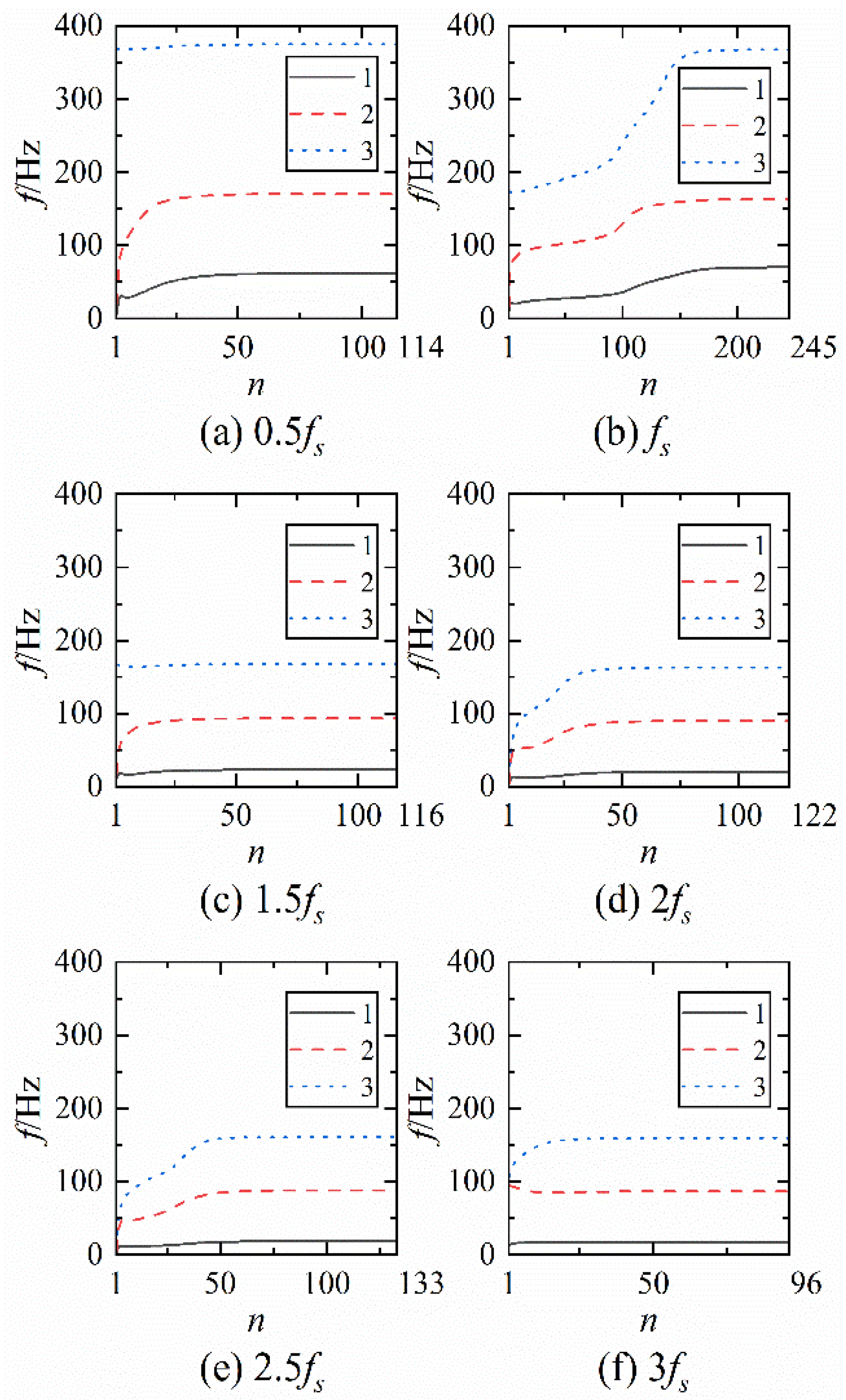
As for signal y, when K = 3, the number of optimal decomposed modal components, α is set as , , , , , and respectively. The curve of the center frequency changes in the modular components after VMD processing is presented in Figure 3 where n denotes the number of iterations while f represents the center frequency of each component.
As presented in Figure 3, when α is set to and , VMD fails to extract the component, that is a frequency of 10 Hz when the iteration is completed. When α is set to , , and , principal frequency, the center frequencies of all modes in the original signal are obtained and the convergence speed gradually slows down and the number of iterations gradually increases. When α is set to , although the original signal is decomposed into three modes with the corresponding center frequencies, the convergence speed becomes faster and the number of iterations becomes smaller. Thus, even if there is same mode number K for VMD method, the selection of different α would make its decomposition performances irregular.
In conclusion, the selection of the mode number K and the penalty factor α affects the VMD decomposition performance and manifest irregularities. When either one of two influencing parameters is maintained unchanged and only the other one is optimized, the interaction between the two parameters could be ignored. This local means of optimization is simple, but it limits the application of the VMD method. To accurately and completely acquire feature information on the milling vibration signal utilizing the VMD method, the DE algorithm is applied to optimize VMD parameters (α and K) simultaneously, and self-adaptively determines the optimal parameter combination.
3. Identification of the Milling Cutter Wear State Based on the Optimized VMD
3.1. Optimization of VMD Parameters Based on DE
During the actual milling process, the feature signal is covered by the environmental noise, especially at the initial wear stage, namely, that the effective signal is weak and the milling cutter wear state is relatively difficult to detect. The feature information of the milling vibration signals is extracted by utilizing the decomposition capacity of the VMD method in the frequency domain. However, the decomposition performance of the VMD method depends on penalty factor α and mode number K. According to subjective judgment, only the relatively optimal parameters could be selected from the finite alternative range, and it is hard to properly choose α and K [36]. To tackle this issue, the optimal parameters of VMD are searched utilizing the global optimization ability of the DE algorithm, thereby leading the population individuals gradually close to the optimal combination of parameters as to imitate the natural evolution process.
The relevant and sensitive signals characterizing the milling cutter wear have periodic cutting chatter information in the time domain signal, which are different from the accidental oscillation in environmental noise. Here, Ep is employed as the objective function to extract periodic feature components. Supposing that the sequence of the signal envelope spectrum amplitudes is , Ep is expressed as follows:
IMF components of the vibration signals collected in the milling process are extracted with the VMD method, in which the more noises are contained, the more characteristics’ information of the milling cutter wear will be covered. Consequently, the periodicity of the component signal is not obvious and the regular impact component cannot be found. In this case, the sparsity of the IMF components is weaker while the Ep is larger. On the contrary, the higher the signal-to-noise ratio of the component signal, the more periodic chatter components associated with the milling cutter wear there are and the smaller the Ep. Given the characteristics of the vibration signals during the milling process, Ep is employed as the objective function of the DE algorithm while Ep minimization is employed as the optimization indicator, and parameter updating is achieved through the evolution operation to search for the optimal parameters of VMD.
The basic principle of the DE algorithm is to randomly generate the initial population within the acceptable range of the variables, from which the parent individuals are chosen and evolved through mutation and cross operation to generate new offspring individuals. Finally, a selecting operation is conducted between parent and offspring individuals to preserve the optimal individuals for the next generation population. Through the continuous evolution of the population, the optimal individual is updated iteratively until convergence occurs and the global optimal individual is obtained. The specific operation steps are presented as follows:
- Initialization;
A vector population is generated, which consists of two-dimensional vectors defined randomly and evenly within the solution space, that are . Herein, the i-th vector in the current population is called an individual in the form of and its element is expressed in the original population () as follows:
where and represent two two-dimensional vectors, the subscripts U and L denote the upper bound and the lower bound respectively, and is a uniformly distributed random quantity within the range of [0, 1).
- 2.
- Mutation;
The mutation operation is to add a scalable and random vector difference component to a third direction quantity to generate a mutation vector as follows:
where F is a scale factor within the range of (0, 1+). F has no upper bound, but its effective value rarely exceeds 1.
- 3.
- Crossover;
After the mutation operation is completed, the vector in each population is crossed with a mutation vector to construct a test vector . The corresponding expression is as follows:
where the crossover probability denotes .
- 4.
- Selection.
The objective function values corresponding to the test vector and the vector are calculated and compared, and the individuals corresponding to the optimal objective function value are selected for the next generation, with the corresponding expression as follows:
Once new populations are generated, the above mutation, crossover, and selection processes are continuously repeated until the iteration stops while the termination criterion is satisfied, thereby yielding an optimal combination of VMD parameters.
3.2. Identification of Sensitive IMF Components Based on the Frequency Domain Cross-Correlation Coefficient
The vibration signals collected during the actual milling process are generally mixed with some noises which seriously interfere with the identification of the milling cutter wear. Although the improved VMD with DE might reduce the noise in the original signal, in fact, the characteristic information of the milling vibration signals could not be fully detected, hence the requirements for the decomposition accuracy may not be met. If some IMF components could reflect the characteristic information of the original signal, they are sensitive IMF, otherwise, they are false IMF. Therefore, determining the sensitive IMF components and superposing them to the reconstruction signal could describe characteristic information of the original signal and further improve the identification accuracy and reliability of the milling cutter wear.
The sensitive IMF component is closely correlated with the original signal since it contains some characteristic information of the original signal. Noises seriously affect the time domain signal analysis, but to analyze a frequency domain thoroughly covered by noise, its power spectral density is small and the peak of the power spectral density of the characteristic information is prominent, therefore, the cross-correlation of the characteristic information power spectral density is less disturbed by noises in the frequency domain. The real sensitive IMF components could filtered out more effectively by using frequency domain cross-correlation than by using the time domain cross-correlation. The sensitive IMF component could be determined utilizing the resultant IMF components and the frequency domain cross-correlation coefficient of the original signal, thus facilitating the analysis and processing of the signal.
Supposing that Kth IMF components is obtained via VMD applied to the original signal , the cross-correlation ρ between and in the frequency domain is expressed as follows:
where and denote the power spectral density corresponding to and respectively while is the sampling frequency.
The frequency domain cross-correlation coefficient ρ is a dimensionless indicator that describes the correlation between the original signal and the decomposed IMF components. , the larger , the stronger the correlation, and vice versa.
Generally, implies weak correlation, and thus the correlation threshold is set to 0.1. The simulation signal y in Equation (8) is processed with VMD by and to extract five IMF components. The time and frequency domain cross-correlation between IMF components and the original signal are calculated, as presented in Figure 4.
As indicated in Figure 4, the time domain cross-correlation coefficient of IMF components varies gently and exceeds the threshold, even including false components, while in frequency domain cross-correlations of IMF4 and IMF5 components are below the threshold; however, the other IMF components are over the threshold. As presented in Figure 2d, IMF1, IMF2, and IMF3 components are the principal frequency components while IMF4 and IMF5 components are false components. Hence, the sensitive IMF components obtained according to cross-correlation in the frequency domain are more consistent with the principal frequency components of the original signal than in the time domain. Therefore, IMF components with the frequency domain cross-correlation coefficient above the threshold are selected for a signal reconstruction that could accurately describe the characteristic information of the original signal.
3.3. Identifying the Milling Cutter Wear Based on the Optimized VMD
Considering the nonlinearity and non-stationary characteristics and strong environmental noises in the vibration signals during milling, this study takes the Ep minimization as the indicator, applies DE to search the optimal parameter combination of VMD, by which the IMF components of the milling vibration signals are obtained, and then reconstructs the vibration signal after sensitive IMF components are sifted out through the frequency domain cross-correlation. Finally, the eigenvalue of the reconstruction signal is extracted and input into the Naive Bayes classifier to identify the milling cutter wear state. The specific implementation steps are as follows:
- Collect vibration signals of the milling cutter at the initial wear, normal wear, and severe wear stages, and measure the worn amount of tool flank;
- Taking the Ep minimization as the assessment indicator, the optimal parameter combination of VMD processing milling vibration signals is found out with DE;
- VMD containing optimal parameter combination is applied to treat the milling vibration signals and acquire K0 IMF components;
- The frequency domain cross-correlation ρ between IMF components and original signals is calculated. If , the IMF component is a sensitive one. Afterward, all sensitive IMF components are superimposed to reconstruct the vibration signal;
- The energy and average amplitude of the reconstruction signals are calculated to obtain the eigenvalues corresponding to the different milling cutter wear states;
- The sample pairs of the extracted eigenvalues and the corresponding milling cutter wear states are trained and tested by the Naive Bayes classifier to identify the milling cutter wear states.
The process of identifying the milling cutter wear state based on the optimized VMD is presented in Figure 5.
4. Experiment and Result Analysis
The cutting experiment was conducted on a vertical CNC milling machine. The workpiece was a block of quenched and tempered 45 steel clamped to the worktable by a vise and its size was 100 mm × 100 mm × 80 mm. The milling cutter was a three-edge high-speed steel end mill with a diameter of 10 mm. The accelerometer (No. 3097A2) made by Dytran Company in the United States was installed on one side of the workpiece, the signal of which was transferred to a laptop through a suited SIRIUSi 8XACC data acquisition board made by Dytran Company in the United States and the sampling rate was set to 1000 Hz. The electron microscope had a 0.7X~5X confocal lens (magnification times of 20X~180X) to take clear pictures of the flank face. Meanwhile, the acoustic emission sensor was fixed on the house of the spindle to collect the sound signal during the milling process, but this signal was not used in this study. The experimental set up is presented in Figure 6.
Due to the inability to control the cutting fluid quantitatively, dry cutting was employed to implement the experiment, in which there were six operation conditions; the cutting parameters are given in Table 1. The tool wear test over a full lifecycle was conducted, in which the tool fed along the X-axis direction of the machine tool with a cutting length of 100 mm. To match the collected vibration signals with the milling cutter wear state, the worn amount of the flank face was measured every 10 cuts until the milling cutter reached its failure.
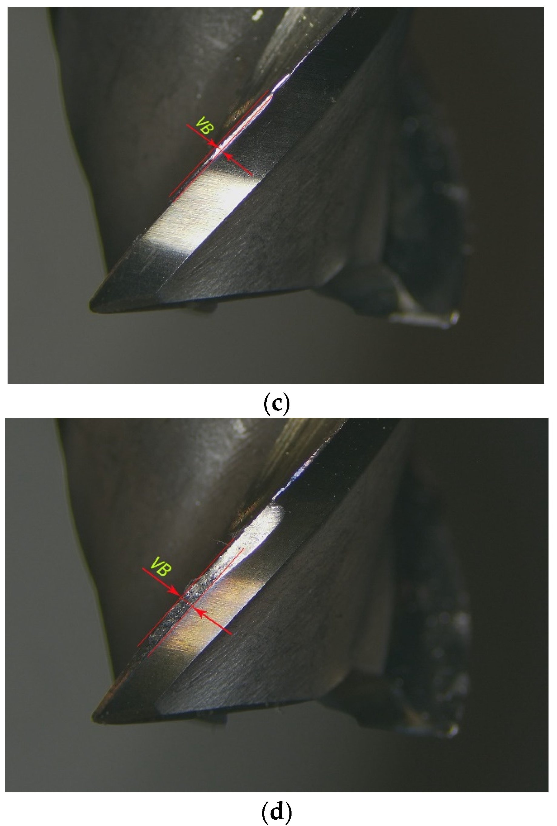
It was relatively convenient to measure the wear loss of the flank face during the actual cutting process, hence the wear degree of the milling cutter was routinely defined according to the average wear width of flank face VB. The average value of the tool wear loss for the three edges was specified as the tool wear loss VB. As for the example of case 1 (Figure 7), the milling cutter wear loss VB below 0.05 mm was at the initial wear stage; that between 0.05~0.3 mm means the normal wear stage and that above 0.3 mm the severe wear stage. The tool wear standard of different stages of the full lifecycle is presented in Figure 8.
Figure 9 displays Z-axis vibration signals collected during the 101st cutting under case 1, where the upper figure is a time domain waveform from accelerometer and the lower figure is its amplitude spectrum.
Little wear information could be observed in the time domain waveform of Figure 9a, and there are few disciplines manifested in Figure 9b. Taking the Ep minimization as an indicator, DE was applied to perform the iterative optimization of VMD parameters [α, K]. The value range for the penalty factor α was [10, 2000] while that for mode number K was in the range of [2,15]. Variation of the objective function value Ep of DE-VMD with the iterations g is shown in Figure 10.
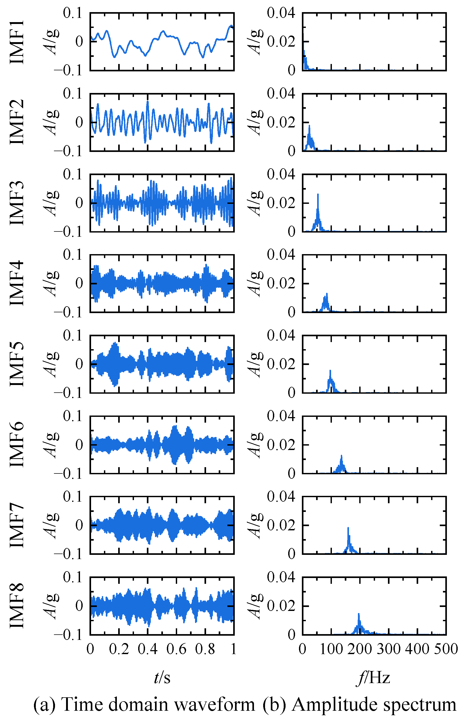
Figure 10 signifies that the convergence of DE-VMD occured at the 29th iteration, and the optimal solution was [1855, 8]. Therefore, VMD processing was conducted on the original signal under the optimal parameters, i.e., . The time domain waveform and amplitude spectrum of each IMF component are presented in Figure 11.
The frequency domain cross-correlations between IMF components and the original signal are presented in Figure 12. As indicated in Figure 12, except for the frequency domain cross-correlation between the IMF7 component and the original signal when below threshold 0.1, the other IMF components exceeding threshold 0.1 were the sensitive ones. Therefore, the IMF7 component was removed while the remaining sensitive IMF components were superimposed to reconstruct the signal. The time domain waveform and amplitude spectrum of the reconstruction signal are presented in Figure 13. The original and reconstruction signals were analyzed utilizing the envelope spectrum, as shown in Figure 14.
Figure 14a demonstrates the envelope spectrum of the original signal. The periodic impact frequency of the vibration signals during the milling process could be observed, but the frequency components of other prominent spectral lines are disordered, which are not the frequency doubling of . The spectral line at each frequency multiplication is not salient. Due to numerous ambient interference spectral lines, it is difficult to detect the frequency multiplier signal of in Figure 14a. Figure 14b is the envelope spectrum of the reconstruction signal, where the spectral amplitude at and its harmonics ~ could be recognized. Notably, the periodic shock signal generated by the milling overwhelmed by the environmental noises is efficiently captured after being processed with the optimized VMD method.
Vibration signals of different wear stages collected in the cutting experiment under six operation conditions were reconstructed through the proposed method, and then the energy and the average amplitude of the reconstruction signals were calculated as the eigenvalue of these vibration signals. Five groups of feature vectors and the corresponding wear stages were randomly selected from each operation condition as the testing dataset while the remaining eigenvectors and the corresponding wear stages were employed as the training dataset. In addition, the Naive Bayes classifier method was applied to calculate the product of the prior probability of each sample type and the posterior probability of each sample in the test set to obtain the probability of each sample type. The type with the maximum probability was selected as the type to which the sample belongs to determine the wear state of the milling cutter.
There were five groups of the testing dataset that were randomly selected for the Naive Bayes classifier. The resultant average identification accuracy of the milling cutter wear stage was used to appraise the extraction performance of the proposed optimized VMD method, which was validated by comparing with EMD and EEMD, as shown in Table 2.
As indicated in Table 2, the present method has a higher level of identification accuracy and could more effectively extract the characteristic information of the milling vibration signals compared with the EMD and EEMD methods. The identification accuracy under different working conditions could reach more than 95%; hence, this method could identify the milling cutter wear state accurately and reliably. The results demonstrate that processing the vibration signals during the milling process through the optimized VMD method could effectively extract the periodic shock signal submerged in the background noises to identify the milling cutter wear state more accurately.
5. Conclusions
Given the difficulty of extracting the milling cutter wear state against the strong background noises, the method of identifying the milling cutter wear state based on the optimized VMD is proposed. The experiment and comparative analysis yield the following conclusions:
- Taking the Ep minimization as an indicator, the DE algorithm is applied to optimize the selection of VMD parameters (α and K), thus effectively tackling the problem of the decomposition effect of VMD being limited by the selection of preset parameters, which is more accurate and reliable than subjective decisions;
- The correlation between respective IMF components obtained from VMD with the optimal parameters and the original signal is analyzed. It is found that the frequency domain cross-correlation coefficient could better filter out the real sensitive IMF components compared with the time domain cross-correlation coefficient. The sensitive IMF components screened by the frequency domain cross-correlation coefficient retain the effective feature information and remove the interference frequency components and therefore could effectively express the characteristic information of the milling vibration signal;
- After the vibration signals are processed through the optimized VMD method, the periodic impact signal submerged in the background noises could be extracted effectively, the eigenvalues of which are trained and tested by Naive Bayesian classification. The results demonstrate that this method could accurately identify the milling cutter wear state under different working conditions. Moreover, compared with EMD and EEMD methods, this method has a higher level of identification accuracy that could effectively extract the characteristic information of the milling vibration signal.
The experimental analysis results indicate that the method of identifying the milling cutter wear state based on the optimized VMD could be employed as an effective scheme for milling cutter wear monitoring to improve milling quality and efficiency. However, it is inadequate to identify three different wear states of the milling cutter by only relying on the optimized VMD method. Therefore, further research and improvements based on the optimized VMD to identify accurate milling cutter wear states are expected.
Author Contributions
Conceptualization, H.C.; methodology, H.C.; software, H.C.; validation, H.C.; formal analysis, H.C.; investigation, H.C.; resources, F.G. and Y.L.; data curation, H.C., F.G., Y.L., X.W., C.G. and L.C.; writing—original draft, H.C.; writing—review and editing, H.C.; visualization, H.C.; supervision, F.G. and Y.L.; project administration, F.G. and Y.L.; funding acquisition, F.G. and L.C. All authors have read and agreed to the published version of the manuscript.
Funding
This research was funded by Key Industrial Innovation Chain Project of Shaanxi Province under grant number 2021ZDLGY-10-07, National Natural Science Foundation of China under grant number 51808038, and Social Science Foundation of Beijing under grant number 18LSC006.
Institutional Review Board Statement
Not applicable.
Informed Consent Statement
Not applicable.
Data Availability Statement
Not applicable.
Conflicts of Interest
The authors declare no conflict of interest.
References
- Yu, W.N.; Mechefske, C.; Kim, I.Y. Identifying optimal features for cutting tool condition monitoring using recurrent neural networks. Adv. Mech. Eng. 2020, 12, 1–14. [Google Scholar] [CrossRef]
- Zhou, Y.Q.; Sun, B.T.; Sun, W.F.; Lei, Z. Tool wear condition monitoring based on a two-layer angle kernel extreme learning machine using sound sensor for milling process. J. Intell. Manuf. 2020, 33, 1–12. [Google Scholar] [CrossRef]
- Xu, X.W.; Wang, J.W.; Ming, W.W.; Chen, M.; An, Q.L. In-process tap tool wear monitoring and prediction using a novel model based on deep learning. Int. J. Adv. Manuf. Technol. 2021, 112, 453–466. [Google Scholar] [CrossRef]
- Shi, M.R.; Qin, X.D.; Li, H.; Shang, S.; Jin, Y.; Huang, T. Cutting force and chatter stability analysis for PKM-based helical milling operation. Int. J. Adv. Manuf. Technol. 2020, 111, 3207–3224. [Google Scholar] [CrossRef]
- Cooper, C.; Wang, P.; Zhang, J.J.; Gao, R.X.; Roney, T.; Ragai, I.; Shaffer, D. Convolutional neural network-based tool condition monitoring in vertical milling operations using acoustic signals. Procedia Manuf. 2020, 49, 105–111. [Google Scholar] [CrossRef]
- Benkedjouh, T.; Zerhouni, N.; Rechak, S. Tool wear condition monitoring based on continuous wavelet transform and blind source separation. Int. J. Adv. Manuf. Technol. 2018, 97, 3311–3323. [Google Scholar] [CrossRef]
- Aralikatti, S.S.; Ravikumar, K.N.; Kumar, H.; Nayaka, H.S.; Sugumaran, V. Comparative study on tool fault diagnosis methods using vibration signals and cutting force signals by machine learning technique. SDHM 2020, 14, 127–145. [Google Scholar] [CrossRef]
- Madhusudana, C.K.; Kumar, H.; Narendranath, S. Condition monitoring of face milling tool using K-star algorithm and histogram features of vibration signal. Eng. Sci. Technol. 2016, 19, 1543–1551. [Google Scholar] [CrossRef] [Green Version]
- Binsaeid, S.; Asfour, S.; Cho, S.; Onar, A. Machine ensemble approach for simultaneous detection of transient and gradual abnormalities in end milling using multisensor fusion. J. Mater. Process. Technol. 2009, 209, 4728–4738. [Google Scholar] [CrossRef]
- Kene, A.P.; Choudhury, S.K. Analytical modeling of tool health monitoring system using multiple sensor data fusion approach in hard machining. Measurement 2019, 145, 118–129. [Google Scholar] [CrossRef]
- Kong, D.D.; Chen, Y.J.; Li, N. Monitoring tool wear using wavelet package decomposition and a novel gravitational search algorithm–least square support vector machine model. Proc. Inst. Mech. Eng. Part C J. Eng. Mech. Eng. Sci. 2020, 234, 822–836. [Google Scholar] [CrossRef]
- Gong, W.G.; Obikawa, T.; Shirakashi, T. Monitoring of tool wear states in turning based on wavelet analysis. JSME Int. J. Ser. C Mech. Syst. Mach. Elem. Manuf. 1997, 40, 447–453. [Google Scholar] [CrossRef] [Green Version]
- Stations, M.; Wu, Y.; Escande, P.; Du, R. A new method for real-time tool condition monitoring in transfer. J. Manuf. Sci. Eng. Trans. ASME 2001, 123, 339–347. [Google Scholar]
- Lin, L.; Wang, B.; Qi, J.J.; Wang, D.; Huang, N.T. Bearing fault diagnosis considering the effect of imbalance training sample. Entropy 2019, 21, 386. [Google Scholar] [CrossRef] [Green Version]
- Huang, J.; Wang, X.Q.; Wang, D.; Wang, Z.W.; Hua, X. Analysis of weak fault in hydraulic system based on multi-scale permutation entropy of fault-sensitive intrinsic mode function and deep belief network. Entropy 2019, 21, 425. [Google Scholar] [CrossRef] [PubMed] [Green Version]
- Cao, W.Q.; Fu, P.; Li, X.H. The diagnosis of tool wear based on EMD and GA-B-spline network. Sens. Transducers 2013, 156, 195–202. [Google Scholar]
- Xu, C.W.; Chai, Y.Z.; Li, H.Y.; Shi, Z.C.; Zhang, L.; Liang, Z.F. A feature extraction method for the wear of milling tools based on the Hilbert marginal spectrum. Mach. Sci. Technol. 2019, 23, 847–868. [Google Scholar]
- Babouri, M.K.; Ouelaa, N.; Djebala, A. Experimental study of tool life transition and wear monitoring in turning operation using a hybrid method based on wavelet multi-resolution analysis and empirical mode decomposition. Int. J. Adv. Manuf. Technol. 2016, 82, 2017–2028. [Google Scholar] [CrossRef]
- Shi, X.H.; Wang, R.; Chen, Q.T.; Shao, H. Cutting sound signal processing for tool breakage detection in face milling based on empirical mode decomposition and independent component analysis. J. Vib. Control 2015, 21, 3348–3358. [Google Scholar] [CrossRef]
- Cao, H.R.; Zhou, K.; Chen, X.F. Chatter identification in end milling process based on EEMD and nonlinear dimensionless indicators. Int. J. Mach. Tools Manuf. 2015, 92, 52–59. [Google Scholar] [CrossRef]
- Wu, Z.H.; Huang, N.E. Ensemble Empirical Mode Decomposition: A noise-assisted data analysis method. Adv. Adapt. Data Anal. 2009, 1, 1–41. [Google Scholar] [CrossRef]
- Amarouayache, I.I.E.; Saadi, M.N.; Guersi, N.; Boutasseta, N. Bearing fault diagnostics using EEMD processing and convolutional neural network methods. Int. J. Adv. Manuf. Technol. 2020, 24, 1–19. [Google Scholar] [CrossRef]
- Jia, Y.C.; Li, G.L.; Dong, X.; He, K. A novel denoising method for vibration signal of hob spindle based on EEMD and grey theory. Measurement 2021, 169, 108490. [Google Scholar] [CrossRef]
- Lei, Y.G.; Liu, Z.Y.; Ouazri, J.; Lin, J. A fault diagnosis method of rolling element bearings based on CEEMDAN. Proc. Inst. Mech. Eng. Part C J. Mech. Eng. Sci. 2017, 231, 1804–1815. [Google Scholar] [CrossRef]
- Tong, S.G.; Zhang, Y.D.; Xu, J.; Cong, F.Y. Pattern recognition of rolling bearing fault under multiple conditions based on ensemble empirical mode decomposition and singular value decomposition. Proc. Inst. Mech. Eng. Part C J. Mech. Eng. Sci. 2018, 232, 2280–2296. [Google Scholar] [CrossRef]
- Dragomiretskiy, K.; Zosso, D. Variational Mode Decomposition. IEEE Trans. Signal Process. 2014, 62, 531–544. [Google Scholar] [CrossRef]
- Liu, C.F.; Zhu, L.D.; Ni, C.B. Chatter detection in milling process based on VMD and energy entropy. Mech. Syst. Signal Proc. 2018, 105, 169–182. [Google Scholar] [CrossRef]
- Liu, C.L.; Tan, J.P.; Huang, Z.H. Fault diagnosis of rolling element bearings based on adaptive mode extraction. Machines 2022, 10, 260. [Google Scholar] [CrossRef]
- Liang, Z.H.; Cao, J.T.; Ji, X.F.; Wei, P. Fault severity assessment of rolling bearings method based on improved VMD and LSTM. J. Vibroeng. 2020, 22, 1338–1356. [Google Scholar]
- Liu, C.; Cheng, G.; Chen, X.H.; Pang, Y.S. Planetary gears feature extraction and fault diagnosis method based on VMD and CNN. Sensors 2018, 18, 1523. [Google Scholar] [CrossRef] [Green Version]
- Li, K.; He, S.P.; Luo, B.; Li, B.; Liu, H.Q.; Mao, X.Y. Online chatter detection in milling process based on VMD and multiscale entropy. Int. J. Adv. Manuf. Technol. 2019, 105, 5009–5022. [Google Scholar] [CrossRef]
- Li, H.; Liu, T.; Wu, X.; Chen, Q. Application of optimized variational mode decomposition based on kurtosis and resonance frequency in bearing fault feature extraction. Trans. Inst. Meas. Control 2020, 42, 518–527. [Google Scholar] [CrossRef]
- Wang, R.; Xu, L.; Liu, F.K. Bearing fault diagnosis based on improved VMD and DCNN. J. Vibroeng. 2020, 22, 1055–1068. [Google Scholar] [CrossRef]
- Zhang, Z.; Li, H.G.; Meng, G.; Tu, X.T.; Cheng, C.M. Chatter detection in milling process based on the energy entropy of VMD and WPD. Int. J. Mach. Tools Manuf. 2016, 108, 106–112. [Google Scholar] [CrossRef]
- Kumar, A.; Zhou, Y.Q.; Xiang, J.W. Optimization of VMD using kernel-based mutual information for the extraction of weak features to detect bearing defects. Measurement 2021, 168, 108402. [Google Scholar] [CrossRef]
- Zhang, H.; Rao, P.; Chen, X.; Xia, H.; Zhang, S.H. Denoising and feature extraction for space infrared dim target recognition utilizing optimal VMD and dual-band thermometry. Machines 2022, 10, 168. [Google Scholar] [CrossRef]
Figure 1.
Simulation signal. (a) Simulation signal y; (b) Simulation signal y1; (c) Simulation signal y2; (d) Simulation signal y3.
Figure 1.
Simulation signal. (a) Simulation signal y; (b) Simulation signal y1; (c) Simulation signal y2; (d) Simulation signal y3.

Figure 2.
Changes of the center frequency with the mode number K. (a) Penalty factor α = 2000, mode number K = 2; (b) Penalty factor α = 2000, mode number K = 3; (c) Penalty factor α = 2000, mode number K = 4; (d) Penalty factor α = 2000, mode number K = 4.
Figure 2.
Changes of the center frequency with the mode number K. (a) Penalty factor α = 2000, mode number K = 2; (b) Penalty factor α = 2000, mode number K = 3; (c) Penalty factor α = 2000, mode number K = 4; (d) Penalty factor α = 2000, mode number K = 4.

Figure 3.
Changes of the center frequency with the penalty factor α. (a) Mode number K = 3, penalty factor α = 500; (b) Mode number K = 3, penalty factor α = 1000; (c) Mode number K = 3, penalty factor α = 1500; (d) Mode number K = 3, penalty factor α = 2000; (e) Mode number K = 3, penalty factor α = 2500; (f) Mode number K = 3, penalty factor α = 3000.

Figure 4.
Cross-correlation in time domain and in frequency domain.

Figure 5.
Flowchart of identifying the milling cutter wear state based on the optimized VMD.

Figure 6.
Experimental set up of milling cutter wear.

Figure 7.
Curve of milling cutter wear.

Figure 8.
Different wear states of milling cutter. (a) New milling cutter; (b) Initial wear; (c) Normal wear; (d) Severe wear.
Figure 8.
Different wear states of milling cutter. (a) New milling cutter; (b) Initial wear; (c) Normal wear; (d) Severe wear.


Figure 9.
Original signal. (a) Time domain waveform of the original signal; (b) Amplitude spectrum of the original signal.
Figure 9.
Original signal. (a) Time domain waveform of the original signal; (b) Amplitude spectrum of the original signal.

Figure 10.
Variation of the objective function value Ep of DE-VMD with the iterations g.

Figure 11.
The IMF components obtained by VMD with the optimal parameters. (a) The time domain waveform of each IMF component; (b) The amplitude spectrum of each IMF component.
Figure 11.
The IMF components obtained by VMD with the optimal parameters. (a) The time domain waveform of each IMF component; (b) The amplitude spectrum of each IMF component.

Figure 12.
Frequency domain cross-correlation between IMF components and original signal.

Figure 13.
Reconstruction signal. (a) Time domain waveform of the reconstruction signal; (b) Amplitude spectrum of the reconstruction signal.
Figure 13.
Reconstruction signal. (a) Time domain waveform of the reconstruction signal; (b) Amplitude spectrum of the reconstruction signal.

Figure 14.
Envelope spectrum of original signal and reconstruction signal. (a) Envelope spectrum of the original signal; (b) Envelope spectrum of the reconstruction signal.
Figure 14.
Envelope spectrum of original signal and reconstruction signal. (a) Envelope spectrum of the original signal; (b) Envelope spectrum of the reconstruction signal.


Table 1.
Milling process parameters.
| Case | ap (mm) | ae (mm) | fz (mm/z) | n (r/min) |
|---|---|---|---|---|
| 1 | 5 | 0.3 | 0.15 | 732 |
| 2 | 4 | 0.3 | 0.07 | 541 |
| 3 | 3 | 0.5 | 0.07 | 732 |
| 4 | 5 | 0.5 | 0.03 | 923 |
| 5 | 4 | 0.4 | 0.03 | 732 |
| 6 | 3 | 0.2 | 0.03 | 541 |
Table 2.
Test results.
| Case | Accuracy | ||
|---|---|---|---|
| EMD | EEMD | Optimized VMD | |
| 1 | 80% | 84% | 96% |
| 2 | 88% | 92% | 96% |
| 3 | 84% | 92% | 100% |
| 4 | 84% | 96% | 96% |
| 5 | 84% | 88% | 100% |
| 6 | 80% | 88% | 96% |
Publisher’s Note: MDPI stays neutral with regard to jurisdictional claims in published maps and institutional affiliations. |
© 2022 by the authors. Licensee MDPI, Basel, Switzerland. This article is an open access article distributed under the terms and conditions of the Creative Commons Attribution (CC BY) license (https://creativecommons.org/licenses/by/4.0/).
Share and Cite
MDPI and ACS Style
Chang, H.; Gao, F.; Li, Y.; Wei, X.; Gao, C.; Chang, L. An Optimized VMD Method for Predicting Milling Cutter Wear Using Vibration Signal. Machines 2022, 10, 548. https://doi.org/10.3390/machines10070548
AMA Style
Chang H, Gao F, Li Y, Wei X, Gao C, Chang L. An Optimized VMD Method for Predicting Milling Cutter Wear Using Vibration Signal. Machines. 2022; 10(7):548. https://doi.org/10.3390/machines10070548
Chicago/Turabian StyleChang, Hao, Feng Gao, Yan Li, Xiaoqing Wei, Chuang Gao, and Lihong Chang. 2022. "An Optimized VMD Method for Predicting Milling Cutter Wear Using Vibration Signal" Machines 10, no. 7: 548. https://doi.org/10.3390/machines10070548
Note that from the first issue of 2016, this journal uses article numbers instead of page numbers. See further details here.