Correlation between Infill Percentages, Layer Width, and Mechanical Properties in Fused Deposition Modelling of Poly-Lactic Acid 3D Printing

Abstract

The field of additive manufacturing (AM) has seen a transformation in the production of intricate and complex parts for various applications. Fused Deposition Modelling (FDM), among AM techniques, has garnered significant attention, particularly in fields like fibre-reinforced composites (FRC). In this study, the world of FDM-printed Polylactic Acid (PLA) components is explored, with a focus on how mechanical properties are influenced by infill percentages and layer widths. Through the utilisation of Response Surface Methodology (RSM), the optimisation of FDM-PLA 3D printing for a wide range of biomaterial applications is achieved, along with the unveiling of the potential for remarkable improvements in mechanical performance. Notably, a remarkable 91% reduction in surface roughness for PLA composites was achieved, accompanied by an impressive 25.6% and 34.1% enhancement in the tensile strength and Young’s modulus of fibre-reinforced PLA composites, respectively. This work, positioned at the crossroads of FDM, lays the groundwork for substantial advancements in the realm of additive manufacturing.

1. Introduction

Fused Deposition Modelling (FDM) has emerged as a transformative force in the realm of 3D printing, offering an economically viable and versatile means to craft intricate objects using thermoplastic polymers [1,2,3,4]. Among these polymers, Polylactic Acid (PLA) has surged in popularity as a renewable resource-derived, biodegradable thermoplastic ideally suited for FDM-based 3D printing [5,6,7]. The appeal of PLA lies in its user-friendly nature, low toxicity, and minimal susceptibility to warping, rendering it a premier choice across diverse applications. Over the years, FDM technology has experienced remarkable advancement, ushering in an era where the creation of complex and functional objects has become effortless [8,9,10]. This innovation, underpinned by the layer-by-layer construction of 3D objects from digital blueprints [11,12,13], has unlocked new horizons spanning aerospace, automotive, medical, and consumer goods sectors [14,15,16].

Particularly noteworthy is PLA’s prominence, attributable to its lower melting point that aligns seamlessly with a wide array of FDM machines [17,18]. The mechanical attributes of FDM-printed PLA components assume pivotal significance, dictating their functional efficacy across engineering and manufacturing landscapes. A nuanced comprehension of the influence wielded by pivotal process parameters on these attributes is indispensable for optimizing the printing process and realizing superior print quality [19]. Prior research endeavors have meticulously explored the intricate interplay between infill percentages [20] and layer widths, unraveling their impact on mechanical characteristics of elastic modulus, tensile strength, elongation at break, tensile extension at the point of tensile strength, and tensile strain at yield [21,22,23]. Integral to these investigations is the employment of Response Surface Methodology (RSM), a statistical approach adept at deciphering multifaceted interactions between variables and their influence on mechanical behavior [24].

Furthermore, researchers have delved into post-processing treatments aimed at elevating the quality of FDM-printed PLA components. Treatments such as annealing and acetone vapor immersion have surfaced as potent techniques, yielding favorable outcomes in domains spanning surface attributes, dimensional fidelity, ductility, and tensile strength [25]. The correction of defects, notably voids, warping, and suboptimal interlayer adhesion, assumes pivotal importance, given their potential to jeopardize the mechanical competence of printed objects [26]. As depicted in Figure 1, the FDM-PLA 3D printing process involves a series of steps that culminate in the creation of innovative designs endowed with improved mechanical properties [27,28].

Enhancements in the mechanical attributes, surface characteristics, and dimensional accuracy of FDM-printed components are attainable through the judicious application of techniques such as laser or acetone vapor treatments [30]. The choice of FDM printing parameters, encompassing layer thickness, infill percentage, and print speed, exert a discernible influence on the mechanical integrity and strength of PLA-fabricated specimens [31]. Optimisation of these parameters has the potential to confer superior tensile strength and toughness. Concomitantly, measures to rectify FDM printing anomalies, including voids, warping, and inadequate interlayer bonding, have been under scrutiny. This endeavor has led to the development of post-processing techniques and the refinement of numerical models, all intended to ameliorate defects and augment the functional properties of printed parts [32]. While Fused Deposition Modelling (FDM) has rapidly ascended as a formidable additive manufacturing technique for fabricating fibre-reinforced composites (FRC), the performance of resultant components often falls short of conventional manufacturing methods, marred by inherent defects [33]. Consequently, concerted efforts have been marshaled to devise treatment methodologies capable of mitigating these shortcomings. This study is rooted in the comprehensive evaluation of the repercussions of these defects on the mechanical competence of FRC and the exploration of remedies to minimize or eradicate these issues, consequently enhancing the functional prowess of printed components. Encompassing both thermoplastic polymers and FRCs actualised via FDM technology, this review encompasses a meticulous analysis of the effects of printing parameters, ranging from layer thickness to infill pattern, raster angle, and fibre orientation. Salient among the defects under scrutiny are void formation, surface irregularities, and suboptimal fibre-matrix bonding. A thoroughgoing discourse ensues on the efficacy of chemical, heat, and ultrasound treatments in ameliorating these issues, culminating in a comprehensive exploration of this treatment landscape [30].

In recent years, the intersection of additive manufacturing and biomaterials has attracted significant attention within the research community. Fused Deposition Modelling (FDM), a popular additive manufacturing technique, has been explored extensively for the fabrication of biomaterial-based structures. Moncayo-Matute et al. [34] conducted a study on the use of FDM to produce patient-specific implants for cranial reconstruction, demonstrating its potential in the medical field. Furthermore, Chalgham et al. [35] investigated the mechanical properties of FDM-printed Polylactic Acid (PLA) composites, highlighting their suitability for orthopedic applications. Building on this foundation, the current study employs Response Surface Methodology (RSM) to optimize FDM-PLA 3D printing, echoing the findings of Portoacă et al. [36] who used similar techniques to enhance the mechanical performance of FDM-printed PLA components. Additionally, Pepelnjak [37] explored the impact of infill percentages and layer widths on FDM-printed parts, providing valuable insights into these critical parameters. As additive manufacturing continues to evolve, the fusion of FDM and biomaterials holds immense promise for advancing personalised medicine and tissue engineering.

In summation, an exhaustive examination of the mechanical attributes intrinsic to biodegradable FDM-PLA 3D printing is undertaken in this article, with a dedicated emphasis on the pivotal roles played by infill percentages and layer widths. The potency of Response Surface Methodology (RSM) is leveraged for a holistic analysis of the intricate interdependence between these variables, thereby illuminating their collective impact. Existing knowledge gaps are bridged with the aim of identifying optimal configurations that bestow heightened mechanical performance upon FDM-printed PLA components. With an in-depth understanding of these decisive parameters, well-informed choices can be made by engineers and designers, thus ensuring the production of high-caliber, dependable FDM-printed PLA components amenable to a multitude of applications.

2. Experimental Design and Methodology

2.1. Response Surface Methodology (RSM)

Response Surface Methodology (RSM) is a statistical approach used to examine the relationship between independent variables and their impact on output variables [38,39]. It allows researchers to manipulate input variables in experiments to understand their influence on the response variable. RSM involves developing a mathematical model based on the experimental data to predict future outcomes [40]. For this study, RSM was chosen due to its capability to handle multiple independent variables and its adaptability to different parameter types. The study focused on infill percentages and layer width as input variables (

Table 1. Input variables for this study with their levels.

Variable	Notation	Unit	−2	−1	0	1	2
Infill Percentages	IP	%	10	20	30	40	50
Width of layer	W	mm	0.4	0.6	0.8	1	1.2

) and identified the most effective parameters as output variables. In this study, Design-Expert v11 was used for modelling. Design-Expert offers a guideline to select a correct power law transformation. It is useful to determine the most appropriate power transformation to apply to response data.

By utilizing RSM, valuable insights were obtained to make informed decisions about the variables and their impact on the overall results. Modulus (GPa), which represents the material’s resistance to deformation, is influenced by the infill percentage and width of the layer. Higher infill percentages result in a denser structure, increasing the modulus. Conversely, a thinner layer width enhances flexibility, leading to a lower modulus. Similarly, % Elongation Tensile Strength at Non-proportional Elongation (Standard) is affected by infill percentage and layer width. Increased infill percentages reduce tensile strength as denser structures are less deformable, while thinner layer widths improve tensile strength by enhancing rigidity. Elongation at Break at Non-proportional Elongation (Standard) follows a similar pattern, with higher infill percentages decreasing elongation due to increased resistance to deformation, while thinner layer widths increase elongation by promoting flexibility. Tensile extension at Tensile Strength and Tensile strain at Yield also demonstrate similar trends, where higher infill percentages reduce extension and strain at yield, while thinner layer widths enhance these properties through increased flexibility.

Table 2. Experimental layout and multi-performance results.

	Input Variables			Output Variables
Experiment No.	Infill Percentages (%)	Width of Layer (mm)	Weight (g)	Modulus (Automatic) (GPa)	% Elongation Tensile Strength at Non-Proportional Elongation (Standard) (%)	Elongation at Break at Non-Proportional Elongation (Standard) (mm)	Tensile Extension at Tensile Strength (mm)	Tensile Strain at Yield (Zero Slope) (mm/mm)
1	30	1.2	10.09	1.43	2.85	5.27	4.70	0.02
2	40	0.6	8.77	1.18	4.83	8.33	7.98	0.04
3	30	0.4	8.03	1.10	6.94	12.05	11.45	0.06
4	30	0.8	8.18	1.26	3.78	6.84	6.24	0.03
5	30	0.8	8.21	1.27	3.82	7.07	6.31	0.03
6	10	0.8	7.25	1.10	4.91	9.10	8.11	0.04
7	50	0.8	9.03	1.31	4.79	8.75	7.91	0.04
8	20	0.6	7.65	1.08	4.80	8.48	7.93	0.04
9	20	1	7.71	1.14	4.50	9.04	7.43	0.04
10	30	0.8	8.34	1.26	0.00	0.00	−4.58	−0.04
11	40	1	8.57	1.35	0.00	0.00	−5.10	−0.01

shows all input/output variables for this study.

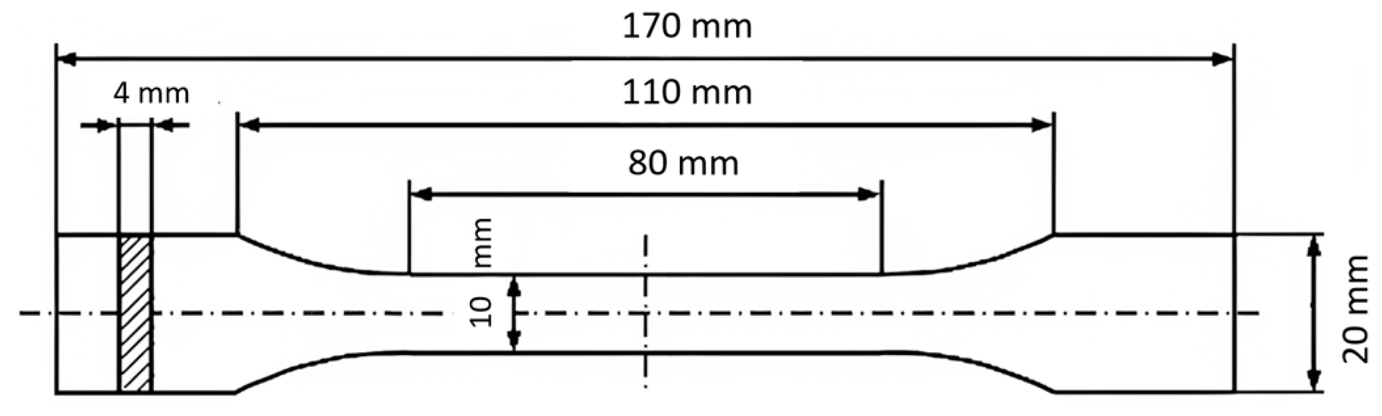
2.2. Material and Dimensional Design Drafting

Polylactic acid (PLA), the material utilised in this study, serves as the initial component and the properties of this material are provided in

Table 3. Properties of polylactic acid for 3D printing [41,42].

Property	Description
Molecular Weight	72.06 g/mol
Melting Point	150–160 °C
Glass Transition Temperature	60–65 °C
Density	1.24–1.26 g/cm3
Refractive Index	1.33–1.53
Young’s Modulus (GPa)	2–4 GPa
Tensile Strength	30–60 MPa
Elongation at Break	5–10%
Impact Strength	5–10 kJ/m2
FDM Printing Temperature Range	190–220 °C
Filament Diameter	1.75 mm or 2.85 mm (common sizes)
Printing Bed Temperature Range	20–60 °C
Biodegradability	Biodegradable under proper conditions

. The PLA was manufactured by 3D FilaPrint (Essex, UK).

The desired shape and dimensions of the specimen are created using computer-aided design (CAD) software SOLIDWORKS. To minimize the impact of stress concentrations caused by loading grips, dog-bone-shaped specimens are recommended for uniaxial tension testing, following the guidelines of ASTM D638 2003 [43].

Once the component design was finalised, the next step involved the selection of constant and variable parameters for the experiment. In order to achieve a comprehensive and statistically significant research project, the principles of the response surface method and the design of experiments (DOE) were employed. The DOE approach permitted the systematic variation of input variables, and data on the response variable of interest were collected correspondingly. A mathematical model in the form of a response surface was created by fitting a polynomial equation to this data.

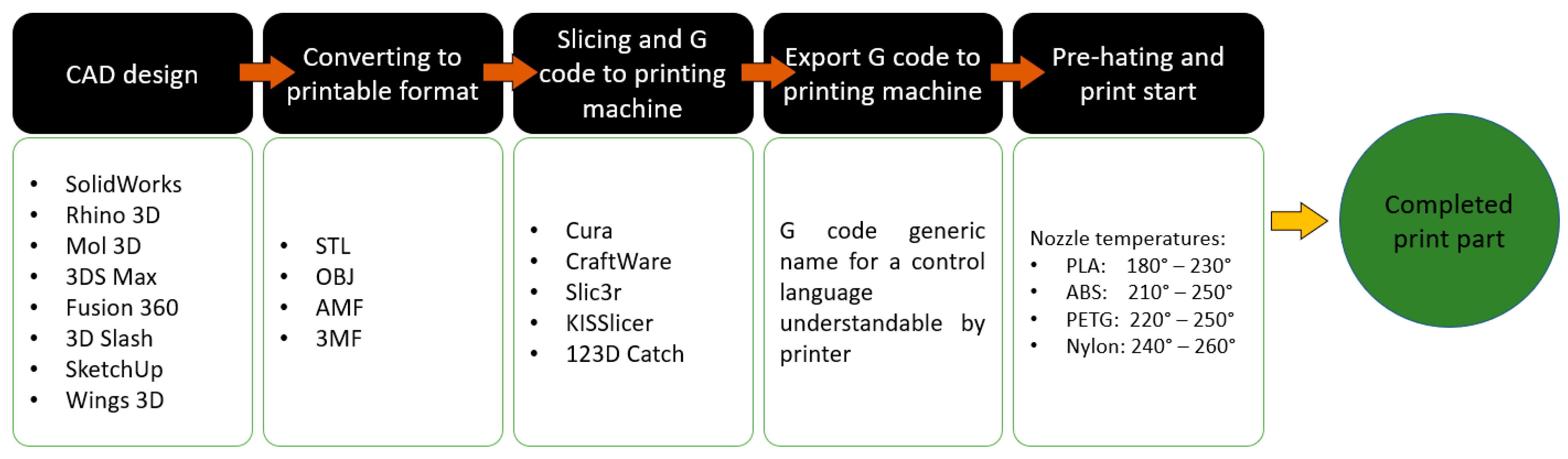
2.3. 3D Printing of the Model

The Ultimaker 3, the 3D printer utilised in this study, features a twin extrusion print head, an auto-nozzle lifting system, swappable print cores, and a filament diameter of 2.85 mm. The printing process is illustrated in Figure 2. The 3D printing process utilised in this study involves a printing apparatus with degrees of freedom in the XYZ direction. This means that the printer is capable of precise movement along three axes: X (horizontal), Y (horizontal), and Z (vertical). This degree of freedom allows for the precise deposition of material layer by layer to create complex three-dimensional objects. On average, the printing process took approximately 45 min to complete a single specimen. This duration includes the time required for material extrusion, layer-by-layer deposition, and any additional processes or settings specific to the experiment. The efficiency and accuracy of the 3D printing apparatus in controlling these movements and parameters were critical to the success of our experiments and the production of high-quality specimens for testing and analysis. In this study, the XY orientation was chosen due to its relevance to the specific objectives of our research. This orientation is commonly used in FDM 3D printing and enables the systematic investigation of the effects of infill percentages and layer widths on mechanical properties. The XY orientation offers a consistent and controlled setup for our experiments, facilitating the comparison of results across different parameter combinations.

A total of 11 specimens were 3D printed, each using specific infill patterns and percentages as specified in the input. All samples were successfully printed, and measurements were obtained. The samples used in this study had dimensions of 170 mm in length, 4 mm in thickness, and a width of 20 mm according to ASTM D638 2003.

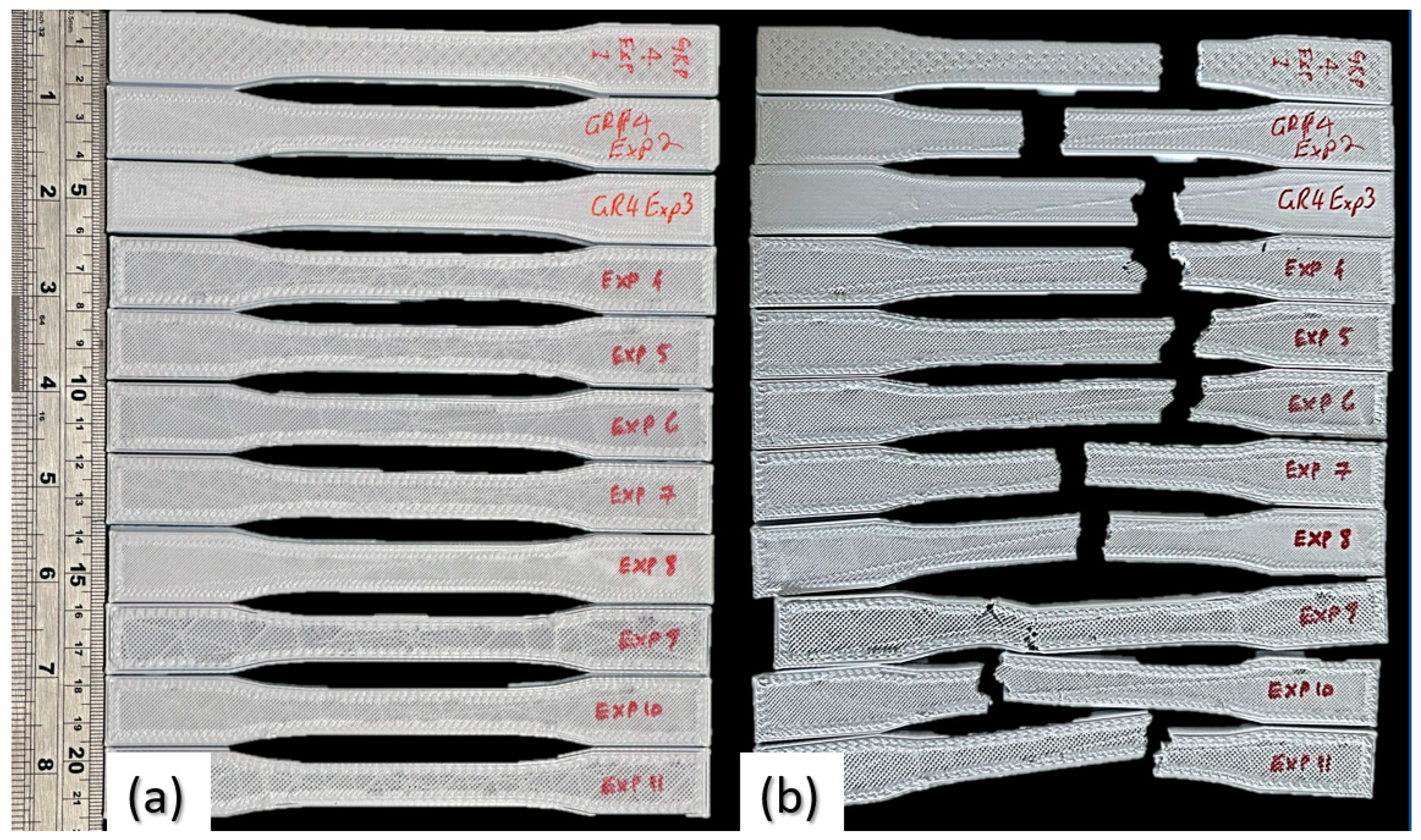
2.4. Tensile Testing

The tensile test experiment was performed to analyze the strength of the specimen. After the printing process, the edges of the specimen were carefully chipped off during post-processing to ensure a consistent and uniform shape for testing. The mechanical properties of the product, including its ultimate tensile strength, elongation at break, and stress-strain behavior, were revealed through the conducted tensile tests. The tensile testing was conducted using a Universal Testing Machine (UTM) equipped with a 5 kN load cell, and the tests were performed at a constant load speed of 1 mm/min (ASTM D638). The test specimen was securely clamped into a Universal Testing Machine (UTM), and a controlled force was gradually applied to stretch the specimen until it reached its breaking point. Throughout the test, continuous measurements and recordings were made of the corresponding elongation and stress values. This data provided insights into the specimen’s mechanical behavior under tension, including its ability to withstand applied forces before failure [44,45]. Additionally, other parameters such as weight and production time were also taken into consideration to evaluate the overall performance of the printed specimens. These factors contributed to the assessment of the specimen’s suitability for specific applications and the efficiency of the 3D printing process. By conducting the tensile test experiment and analyzing the data collected, a deeper understanding of the mechanical properties and performance of the printed PLA specimens can be gained [46,47]. This information is crucial for optimizing the design, material selection, and manufacturing parameters in FDM-PLA 3D printing processes. Figure 3 shows the geometrical dimensions of tensile test samples.

3. Results and Discussion

Table 2 presents the experimental layout and multi-performance results obtained from the conducted experiments. The input variables include infill percentages (%) and the width of the layer (mm), while the output variables comprise various performance indicators. Experiment No. 1 utilised an infill percentage of 30%, and a layer width of 1.2 mm, resulting in a weight of 10.09 g. The corresponding performance results include a modulus (automatic) of 1.436 GPa, a % elongation of 2.85 at non-proportional elongation, an elongation at break of 5.27 mm at non-proportional elongation, a tensile extension of 4.70 mm at the tensile strength, and a tensile strain of 0.02 mm/mm at yield. Similar analyses were carried out for the remaining experiments, with different combinations of infill percentages and layer widths. The corresponding performance results for each experiment provide insights into the mechanical behavior and characteristics of the printed specimens, including modulus, elongation, tensile strength, and strain at various points. Figure 4 shows the 3D-printed specimens before and after the tensile test.

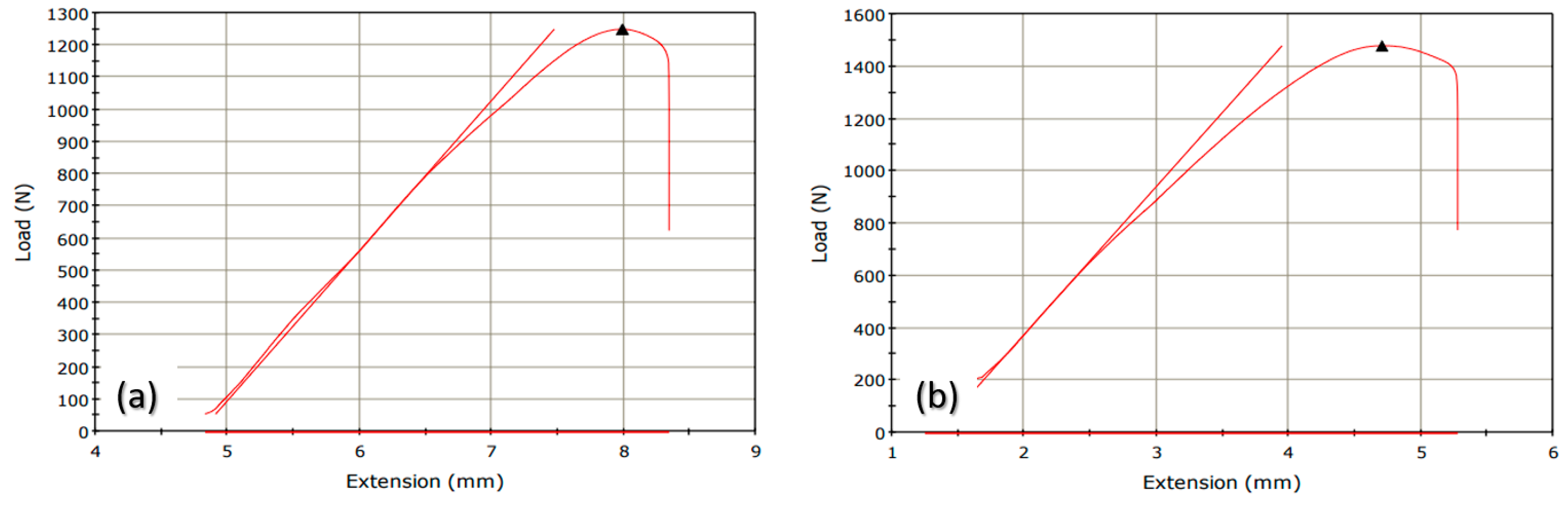
3.1. Tensile Test Result

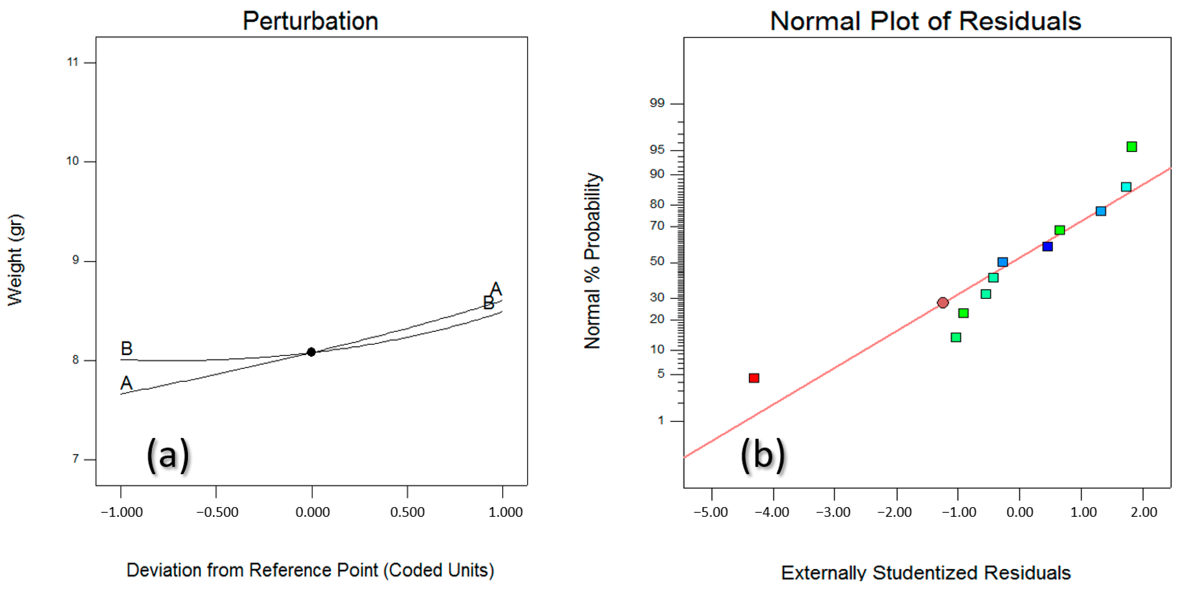
The experimental results obtained from the tensile tests are presented in

Table 4. High-performing and low-performing specimens at tensile test results.

Output Variables	High-Performing Value	Experiment No.	Low-Performing Value	Experiment No.
Modulus (Automatic) (GPa)	1.43	1	1.26	10
% Elongation Tensile Strength at Non-proportional Elongation (Standard) (%)	6.94	3	0.00	10
Elongation at Break at Non-proportional Elongation (Standard) (mm)	12.05	3	0.00	10
Tensile extension at Tensile Strength (mm)	9.10	6	−4.58	10
Tensile strain at Yield (Zero Slope) (mm/mm)	0.04	9	−0.08	10

. The table includes the input variables, which are the infill percentages and width of the layer, and the corresponding output variables, which consist of various mechanical properties. Upon analyzing the data, several observations can be made.

First, the infill percentage seems to have an impact on the mechanical properties of the samples. For example, as the infill percentage increases from 10% to 50%, there is a general trend of increased modulus, indicating greater stiffness and resistance to deformation. However, it is noteworthy that in Experiment 10 and Experiment 11, where the infill percentage is fixed at 30% and 40%, the tensile strength and elongation values drop to zero, suggesting a limitation or other factors affecting the properties in these specific cases. Second, the width of the layer also plays a role in determining the mechanical behavior of the samples. Generally, a thinner width of the layer results in higher values for tensile strength, elongation at break, and tensile extension. This suggests that a thinner layer provides increased rigidity and strength to the material, allowing it to withstand higher loads before failure. It is important to note that some of the experiments have negative values for tensile extension and tensile strain at yield, namely Experiment 10 and Experiment 11. These negative values as shown in Figure 5 indicate a deviation from the expected behavior and might be attributed to experimental limitations or measurement errors.

3.2. Weight

The analysis of variance (ANOVA)

Table 5. ANOVA for Response Surface Reduced Quadratic model for weight.

Source	Sum of Squares	df	Mean Square	F-Value	p-Value
Model	1.796 × 10−6	3	5.988 × 10−7	15.88	0.0017
A-IP	1.252 × 10−6	1	1.252 × 10−6	33.21	0.0007
B-LW	2.887 × 10−7	1	2.887 × 10−7	7.66	0.0278
B2	2.555 × 10−7	1	2.555 × 10−7	6.78	0.0353
Residual	2.639 × 10−7	7	3.771 × 10−8
Lack of Fit	2.580 × 10−7	5	5.159 × 10−8	17.24	0.0557
Pure Error	5.986 × 10−9	2	2.993 × 10−9
Cor Total	2.060 × 10−6	10
			R-Squared = 87.19%		Adj R-Squared = 81.79%

for the Response Surface Reduced Quadratic model provides insights into the significance of the model and its individual factors. The table displays the sums of squares, degrees of freedom, mean squares, F-values, and p-values for each source. The model as a whole shows a significant effect on the response variable, as indicated by the p-value of 0.0017. This suggests that the model is a good fit for the data and can explain a significant portion of the variation in the response variable. Breaking down the individual factors, the factor A-IP (infill percentages) demonstrates a highly significant effect with a p-value of 0.0007. This suggests that infill percentages have a significant impact on the response variable. The factor B-LW (layer width) also shows a significant effect with a p-value of 0.02. This indicates that layer width plays a role in influencing the response variable. The factor B2, representing the squared term for layer width, is also significant with a p-value of 0.03. This suggests that the relationship between layer width and the response variable is not linear, but rather has a quadratic effect. The residual sum of squares represents the variation in the response variable that is not accounted for by the model. The lack of fit sum of squares, which compares the model’s fit to the replicated data, is not significant with a p-value of 0.05. This indicates that the model adequately fits the data, and the remaining variation can be attributed to random error. The adj R-Squared value of 0.81 indicates that the model explains approximately 81.79% of the total variation in the response variable. This indicates a good fit of the model to the data.

Equation (1) provided relates the response variable (weight) to the factors A-IP (infill percentages), B-LW (layer width), and B² (squared layer width). The coefficients accompanying each factor indicate the magnitude and direction of their impact on the response variable. For example, a positive coefficient suggests a positive effect on the response variable, while a negative coefficient indicates a negative effect.

(Weight)⁻³ = +1.80863 × 10⁻³ − 3.23027 × 10⁻⁵ × IP + 3.44918 × 10⁻³ × LW − 2.64042 × 10⁻³ × LW²

(1)

The normal plots of residuals are used to assess the normality of the residuals, which are the differences between the observed and predicted values of the response variable. When A and B have a relationship and intersect, it can affect the distribution of residuals. The normal plots of residuals provide a graphical representation of how well the residuals follow a normal distribution. Departures from normality in the plots may indicate the presence of interactions between A and B. Analyzing the perturbation plot and normal plots of residuals when A and B intersect allows researchers to understand the complex relationship between these variables and their impact on the response variable. It helps in identifying the regions where A and B have significant effects on the response, as well as regions where their interaction is more pronounced (Figure 6).

3.3. Modulus

The ANOVA

Table 6. ANOVA for Response Surface Linear model for modulus.

Source	Sum of Squares	df	Mean Square	F-Value	p-Value
Model	1.699 × 10−4	2	8.496 × 10−5	21.58	0.0006
A-IP	7.578 × 10−5	1	7.578 × 10−5	19.25	0.0023
B-LW	9.414 × 10−5	1	9.414 × 10−5	23.91	0.0012
Residual	3.149 × 10−5	8	3.937 × 10−6
Lack of Fit	3.131 × 10−5	6	5.219 × 10−6	58.23	0.0170
Pure Error	1.793 × 10−7	2	8.963 × 10−8
Cor Total	2.014 × 10−4	10
			R-Squared = 84.36%		Adj R-Squared = 80.46%

for the Response Surface Linear model provides insights into the significance of the model and its individual factors. The table displays the sums of squares, degrees of freedom, mean squares, F-values, and p-values for each source. The model as a whole shows a significant effect on the response variable, as indicated by the p-value of 0.0006. This suggests that the linear model is a good fit for the data and can explain a significant portion of the variation in the response variable. Analyzing the individual factors, both factor A-IP (infill percentages) and factor B-LW (layer width) demonstrate significant effects on the response variable, with p-values of 0.0023 and 0.0012, respectively. This suggests that both infill percentages and layer width have a significant impact on the response variable. The residual sum of squares represents the variation in the response variable that is not accounted for by the model. The lack of fit sum of squares compares the model’s fit to the replicated data. In this case, the lack of fit is significant with a p-value of 0.0170. This indicates that the linear model does not adequately capture all the variation in the data, and there is additional unexplained variability present. The Adj R-Squared value of 0.8046 indicates that the model explains approximately 80.46% of the total variation in the response variable. This suggests a reasonably good fit of the linear model to the data.

The Equation (2) provided relates the response variable (modulus) to the factors A-IP (infill percentages) and B-LW (layer width). The coefficients accompanying each factor indicate the magnitude and direction of their impact on the response variable. A positive coefficient suggests a positive effect on the response variable, while a negative coefficient indicates a negative effect.

(Modulus)^−1.32 = +0.055579 − 2.51305 × 10⁴ × IP − 0.14005 × LW

(2)

The Box-Cox plot in Figure 7 is a powerful tool for analyzing the relationship between input variables A and B and their effects on the responses. It specifically focuses on examining the transformation of the response variable using different values of the lambda parameter. In this analysis, when the lambda value is set to −1.34, this suggests that there is a nonlinear relationship between A and B and the response variable. The transformation helps to improve the linearity of the relationship and can potentially lead to better model fit and interpretation. The increase in the natural logarithm of the residuals indicates that the original response variable may have been skewed or heteroscedastic, meaning the variability of the response changes with the level of A and B. By applying the Box-Cox transformation with lambda equal to −1.34, we are able to address these issues and obtain more reliable and accurate results. It is important to note that selecting the appropriate value of lambda is crucial to achieving the desired transformation. The value of −1.34 was determined to be the optimal choice based on the observed increase in the Ln (residuals). However, it is essential to consider other diagnostic tools, such as residual plots and statistical tests, to validate the adequacy of the chosen transformation and ensure its appropriateness for the specific data set.

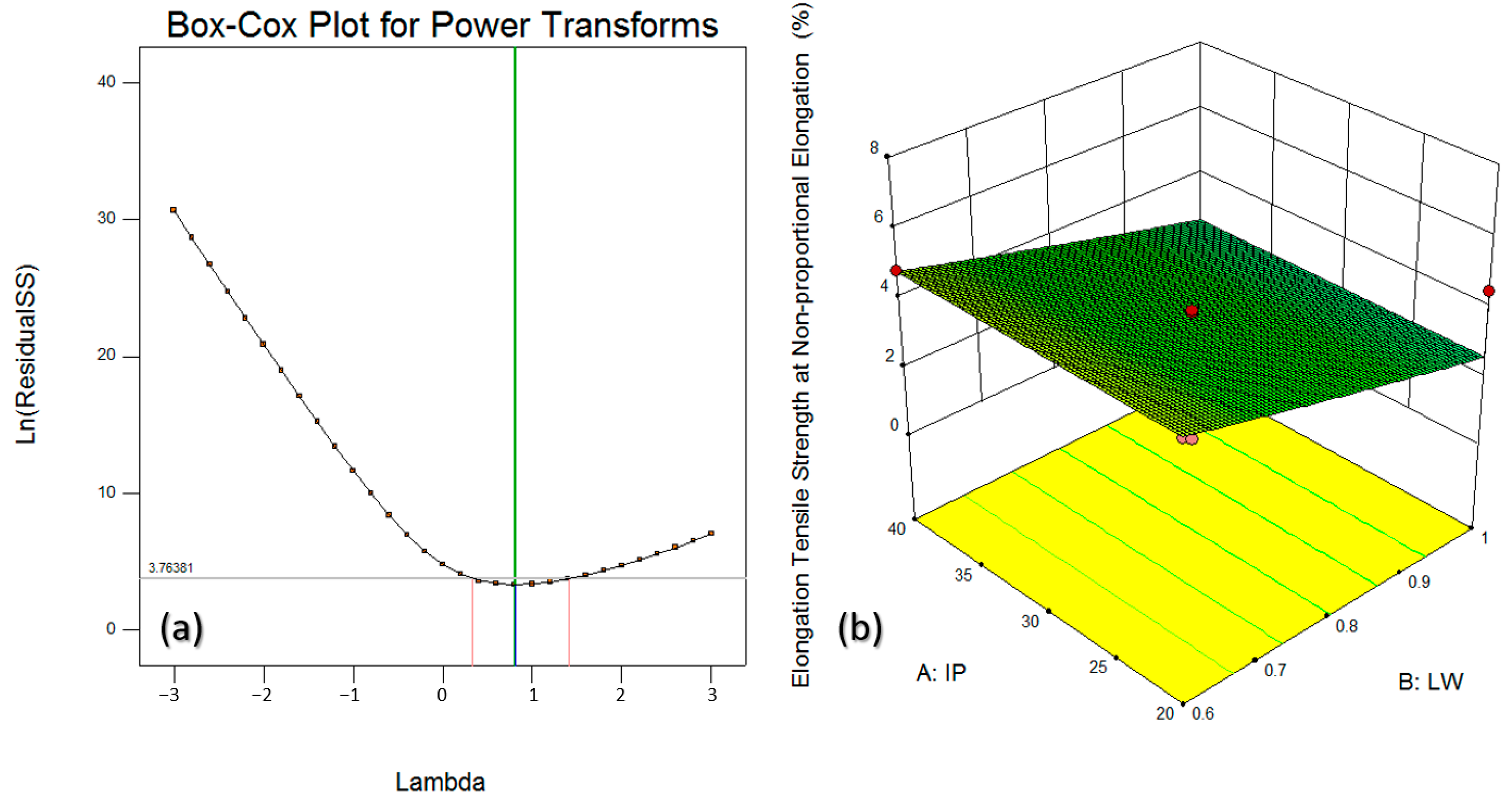
3.4. Elongation Tensile Strength at Non-Proportional Elongation

The ANOVA

Table 7. ANOVA for Response Surface Reduced Linear model for Elongation Tensile Strength at Non-proportional Elongation.

Source	Sum of Squares	df	Mean Square	F-Value	p-Value
Model	6.31	1	6.31	3.45	0.0962
B-LW	6.31	1	6.31	3.45	0.0962
Residual	16.47	9	1.83
Lack of Fit	10.66	7	1.52	0.52	0.7820
Pure Error	5.81	2	2.91
Cor Total	22.78	10
			R-Squared = 27.71%		Adj R-Squared = 19.68%

for the Response Surface Reduced Linear model provides insights into the significance of the model and its individual factors. The table displays the sums of squares, degrees of freedom, mean squares, F-values, and p-values for each source. In this case, the model as a whole does not show a significant effect on the response variable, as indicated by the p-value of 0.0962. This suggests that the reduced linear model may not be a good fit for the data, and it does not explain a significant portion of the variation in the response variable. Analyzing the individual factor, B-LW (layer width), it also does not show a significant effect on the response variable, as indicated by the p-value of 0.0962. This suggests that the layer width may not have a significant impact on the response variable based on this model. The residual sum of squares represents the variation in the response variable that is not accounted for by the model. The lack of fit sum of squares compares the model’s fit to the replicated data. In this case, the lack of fit is not significant with a p-value of 0.7820. This indicates that the reduced linear model adequately captures the variation in the data, and the remaining variation can be attributed to random error. The R-squared value of 0.1968 indicates that the model explains approximately 19.68% of the total variation in the response variable. This suggests that the reduced linear model has a limited ability to explain the variation in the data.

Equation (3) relates the response variable (elongation tensile strength at non-proportional elongation) to the factor B-LW (layer width). The coefficient accompanying the factor indicates the magnitude and direction of its impact on the response variable. A positive coefficient suggests a positive effect on the response variable, while a negative coefficient indicates a negative effect.

(Elongation Tensile Strength at Non-proportional Elongation)^0.81 = + 5.69899 − 3.62634 × LW

(3)

In the Box-Cox plot (Figure 8a), the response variable is transformed for different lambda values. Optimal lambda value selection aims to maximize linearity and normality in the relationship. The analysis shows that as B:LW is increased, there is a reduction in the Elongation Tensile Strength at Non-proportional Elongation. By examining the Box-Cox plot, the most appropriate lambda value can be determined to achieve a more linear relationship and enhance the model’s fit.

The surface plot (Figure 8b) presents a visual representation of how the Elongation Tensile Strength at Non-proportional Elongation changes as B:LW increases. It illustrates the variation in the response across different levels of B:LW. The surface plot allows observation of the direction and magnitude of the response’s change with increasing B:LW, indicating that an increase in B:LW is associated with a decrease in the Elongation Tensile Strength at Non-proportional Elongation. The combined insights from the Box-Cox plot and surface plot indicate that the Elongation Tensile Strength at Non-proportional Elongation is affected by the increase in B:LW. If necessary, applying the Box-Cox transformation can further improve linearity and normality, enhancing the accuracy and reliability of the model.

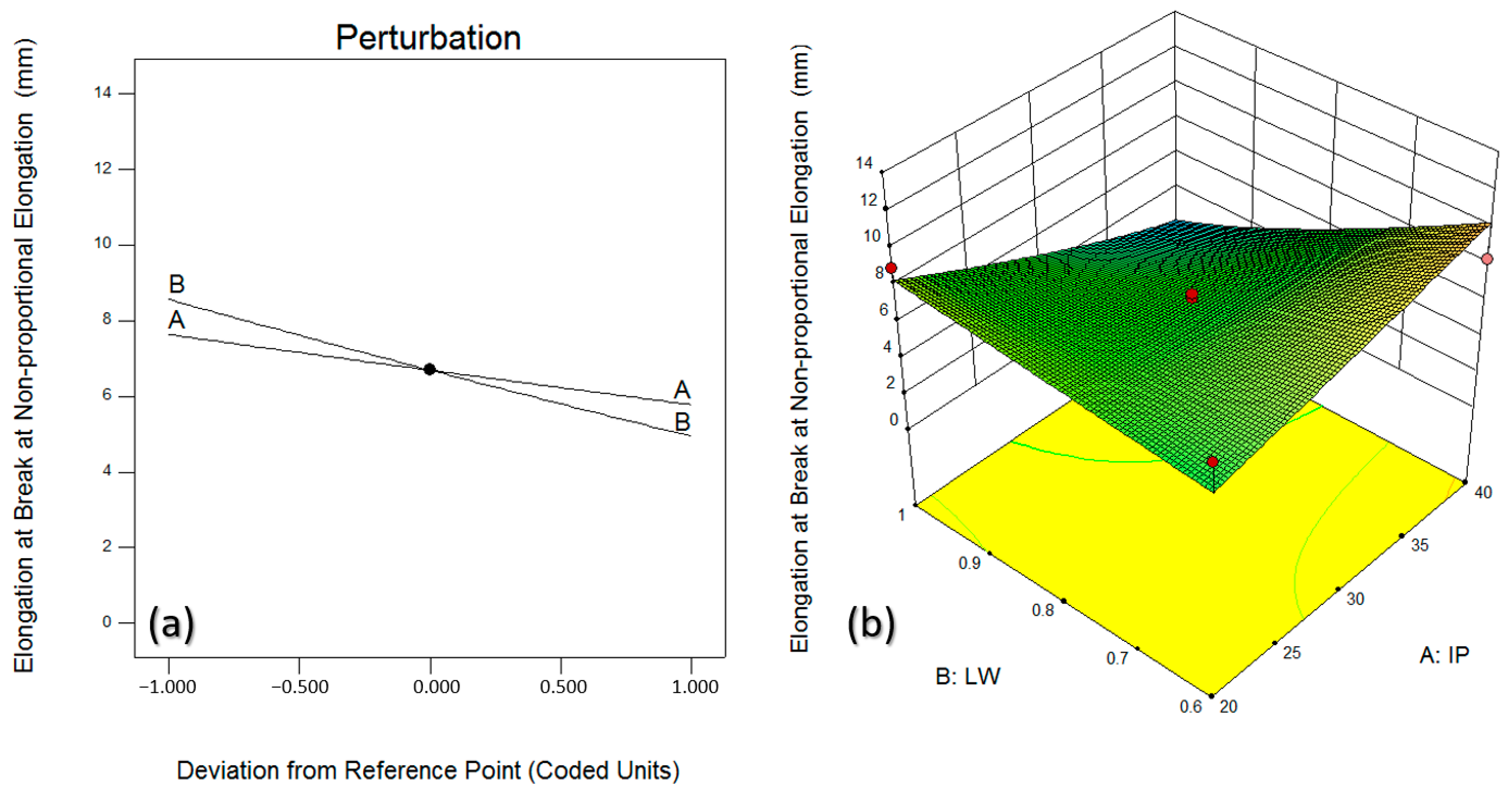
3.5. Elongation at Break at Non-Proportional Elongation

The ANOVA

Table 8. ANOVA for Response Surface 2FI model for Elongation at Break at Non-proportional Elongation.

Source	Sum of Squares	df	Mean Square	F-Value	p-Value
Model	24.05	3	8.02	1.76	0.2429
A-IP	3.27	1	3.27	0.72	0.4257
B-LW	12.53	1	12.53	2.74	0.1417
AB	8.26	1	8.26	1.81	0.2207
Residual	31.98	7	4.57
Lack of Fit	17.10	5	3.42	0.46	0.7909
Pure Error	14.88	2	7.44
Cor Total	56.03	10
			R-Squared = 42.93%		Adj R-Squared = 18.47%

for the Response Surface 2FI model provides insights into the significance of the model and its individual factors. The table displays the sums of squares, degrees of freedom, mean squares, F-values, and p-values for each source. In this case, the model as a whole does not show a significant effect on the response variable, as indicated by the p-value of 0.2429. This suggests that the 2FI model may not be a good fit for the data, and it does not explain a significant portion of the variation in the response variable. Analyzing the individual factors, A-IP (infill percentages), B-LW (layer width), and AB (interaction between infill percentages and layer width) do not show significant effects on the response variable, as indicated by their respective p-values of 0.4257, 0.1417, and 0.2207. This suggests that these factors may not have a significant impact on the response variable based on this model. The residual sum of squares represents the variation in the response variable that is not accounted for by the model. The lack of fit sum of squares compares the model’s fit to the replicated data. In this case, the lack of fit is not significant with a p-value of 0.7909. This indicates that the 2FI model adequately captures the variation in the data, and the remaining variation can be attributed to random error. The R-squared value of 0.1847 indicates that the model explains approximately 18.47% of the total variation in the response variable. This suggests that the 2FI model has a moderate ability to explain the variation in the data and the previous research studies also confirmed [48].

The equation provided relates the response variable (elongation at break at non-proportional elongation) to the factors A-IP (infill percentages), B-LW (layer width), and their interaction term AB. The coefficients accompanying each factor indicate the magnitude and direction of their impact on the response variable. Positive coefficients suggest a positive effect on the response variable, while negative coefficients indicate a negative effect (Equation (4)).

(Elongation at Break at Non-proportional Elongation)^0.8 = −7.14477 + 0.52254 × IP + 16.44353 × LW − 0.71840 × IP × LW

(4)

The perturbation analysis was conducted to investigate the effects of varying the input variables A:IP and B:WL on the response variable Elongation at Break at Non-proportional Elongation (Figure 9a). By systematically perturbing the levels of A:IP and B:WL while keeping other factors constant, the sensitivity of the response to changes in these variables was assessed. The analysis reveals that increasing A:IP and decreasing B:WL have a significant impact on reducing the Elongation at Break at Non-proportional Elongation. As A:IP increases, and B:WL decreases, the response variable shows a consistent decrease. This indicates that higher levels of A:IP and lower levels of B:WL result in a decreased ability of the material to elongate before reaching the point of breakage.

The surface plot provides a visual representation of how the Elongation at Break at Non-proportional Elongation changes with varying levels of A:IP and B:WL. The plot shows a downward trend as A:IP increases and B:WL decreases, indicating a decrease in the Elongation at Break at Non-proportional Elongation. The surface plot displays a contoured surface that represents the response variable as a function of the two input variables. It allows us to observe the combined effects of A:IP and B:WL on the Elongation at Break at Non-proportional Elongation. The plot demonstrates that higher A:IP and lower B:WL values lead to a reduced Elongation at Break at Non-proportional Elongation (Figure 9b).

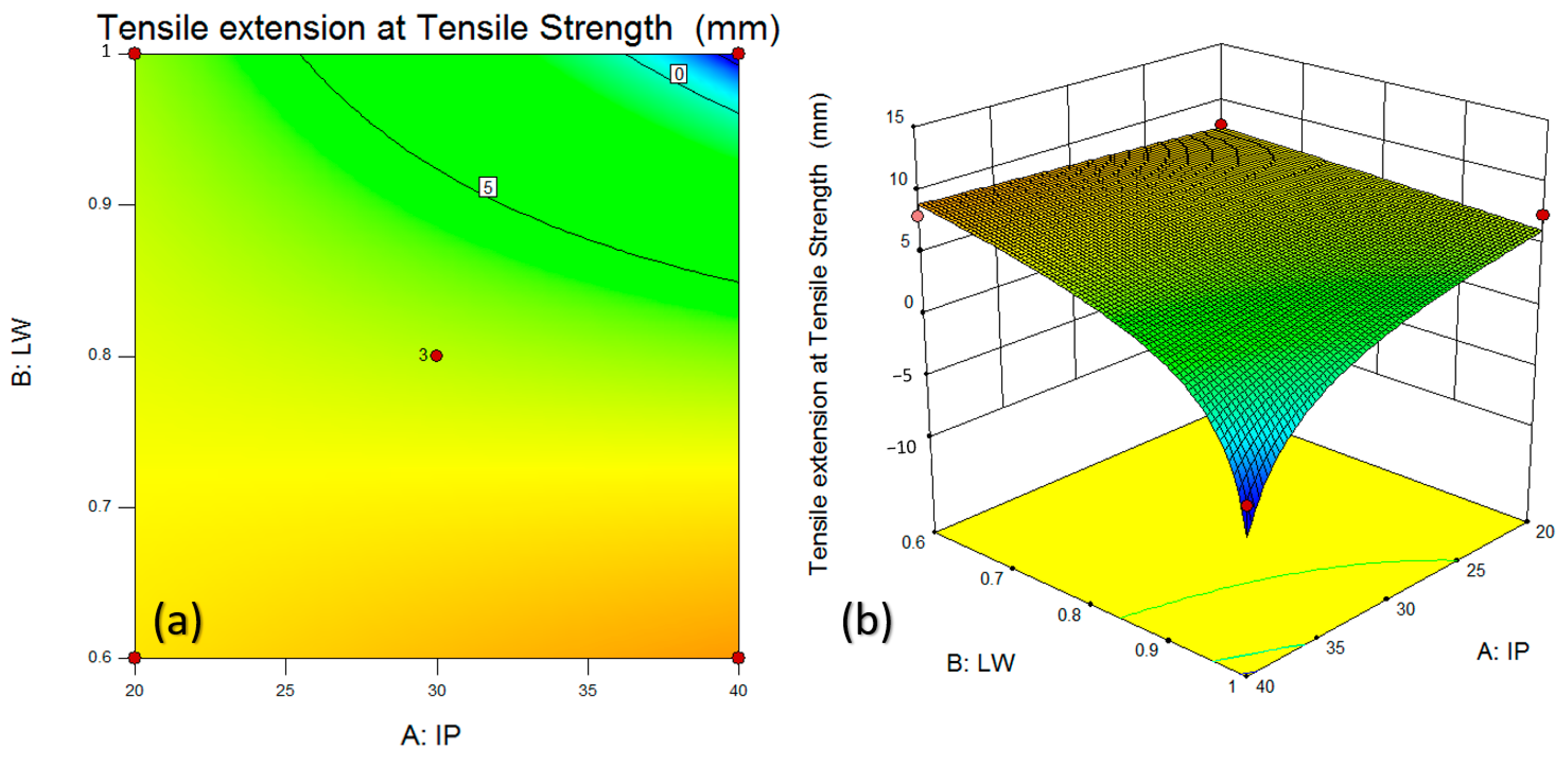
3.6. Tensile Extension at Tensile Strength

The ANOVA

Table 9. ANOVA for Response Surface 2FI model Tensile extension at Tensile Strength.

Source	Sum of Squares	df	Mean Square	F-Value	p-Value
Model	9.210 × 106	3	3.070 × 106	3.27	0.0889
A-IP	3.873 × 105	1	3.873 × 105	0.41	0.5409
B-LW	7.821 × 106	1	7.821 × 106	8.34	0.0234
AB	1.002 × 106	1	1.002 × 106	1.07	0.3357
Residual	6.564 × 106	7	9.377 × 105
Lack of Fit	5.109 × 106	5	1.022 × 106	1.40	0.4656
Pure Error	1.455 × 106	2	7.277 × 105
Cor Total	1.577 × 107	10
			R-Squared = 58.39%		Adj R-Squared = 40.55%

for the Response Surface 2FI model provides insights into the significance of the model and its individual factors. The table displays the sums of squares, degrees of freedom, mean squares, F-values, and p-values for each source. In this case, the model as a whole does not show a significant effect on the response variable, as indicated by the p-value of 0.0889. This suggests that the 2FI model may not be a good fit for the data, and it does not explain a significant portion of the variation in the response variable. Analyzing the individual factors, A-IP (infill percentages) and AB (interaction between infill percentages and layer width) do not show significant effects on the response variable, as indicated by their respective p-values of 0.5409 and 0.3357. This suggests that these factors may not have a significant impact on the response variable based on this model. However, the factor B-LW (layer width) does show a significant effect on the response variable, as indicated by its p-value of 0.0234. This suggests that layer width may have a significant impact on the response variable based on this model. The residual sum of squares represents the variation in the response variable that is not accounted for by the model. The lack of fit sum of squares compares the model’s fit to the replicated data. In this case, the lack of fit is not significant with a p-value of 0.4656. This indicates that the 2FI model adequately captures the variation in the data, and the remaining variation can be attributed to random error. The R-squared value of 0.4055 indicates that the model explains approximately 40.55% of the total variation in the response variable.

Equation (5) provided relates the response variable (tensile extension at tensile strength + 5.11) to the factors A-IP, B-LW, and their interaction term AB. The coefficients accompanying each factor indicate the magnitude and direction of their impact on the response variable. Positive coefficients suggest a positive effect on the response variable, while negative coefficients indicate a negative effect.

(Tensile extension at Tensile Strength + 5.11)³ = −473.17680 + 182.21420 × IP + 3470.22079 × LW − 250.22556 × IP × LW

(5)

Figure 10 illustrates the relationship between the input variables B:LW and A:IP and their impact on the response variable Tensile extension at Tensile Strength. The contour plot showcases the contours of Tensile extension at Tensile Strength with varying levels of B:LW and A:IP. The contour lines connect points of equal Tensile extension at Tensile Strength, allowing us to visualize the interaction between the two input variables and the resulting response [49].

From the contour plot, it can be observed that increasing both B:LW and A:IP leads to a reduction in Tensile extension at Tensile Strength. The contour lines are more closely spaced and exhibit a downward trend as the levels of B:LW and A:IP increase. This indicates that higher values of B:LW and A:IP result in a decrease in the Tensile extension at Tensile Strength. The surface plot provides a three-dimensional representation of the relationship between B:LW, A:IP, and Tensile extension at Tensile Strength. It allows us to visualize the response variable as a function of the two input variables in a more detailed manner. The surface plot reveals a clear downward trend as both B:LW and A:IP increase. As B:LW increases along the x-axis and A:IP increases along the y-axis, the surface plot demonstrates a decreasing trend in Tensile extension at Tensile Strength. The surface becomes progressively lower as the values of B:LW and A:IP increase, indicating a reduction in Tensile extension at Tensile Strength.

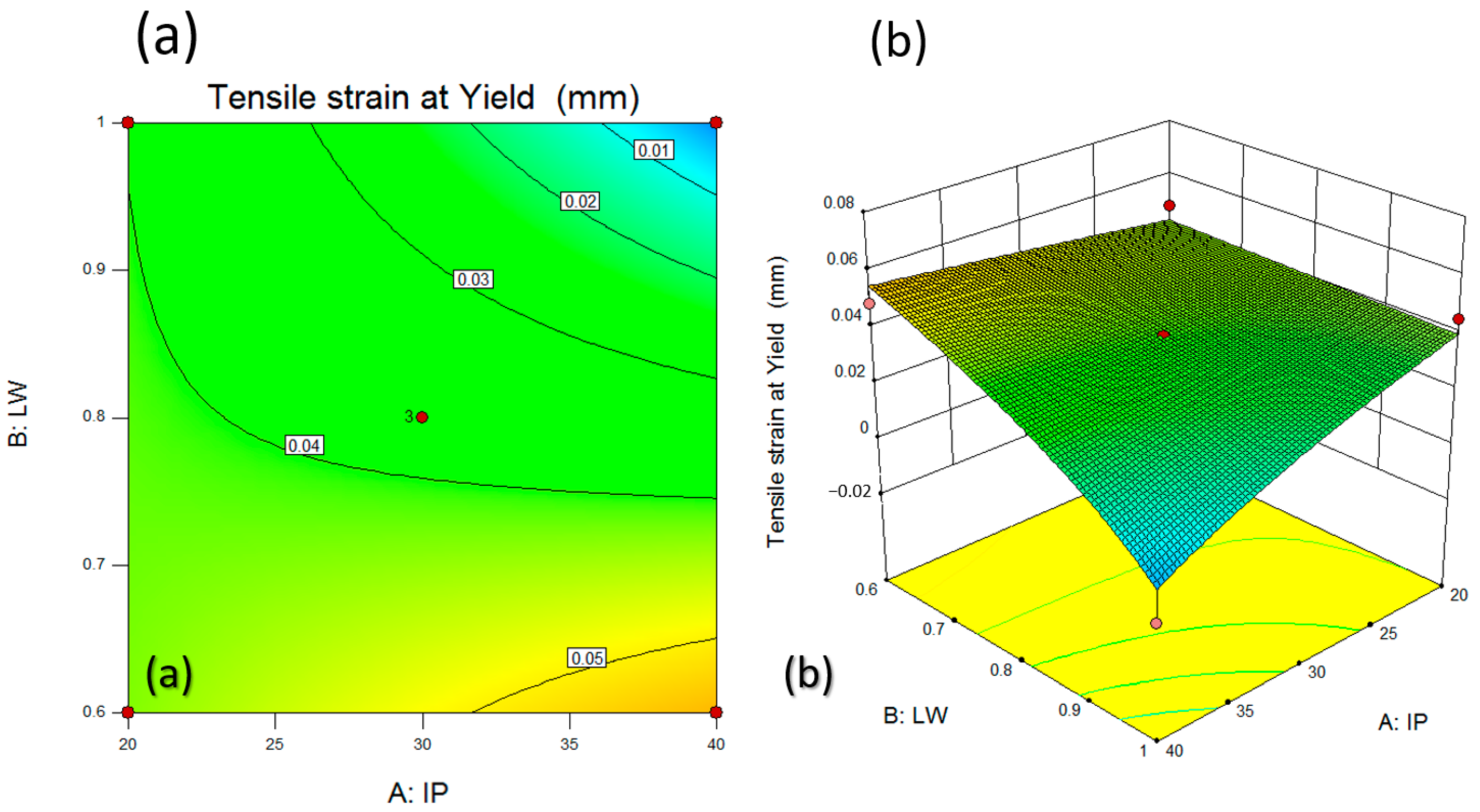
3.7. Tensile Strain at Yield

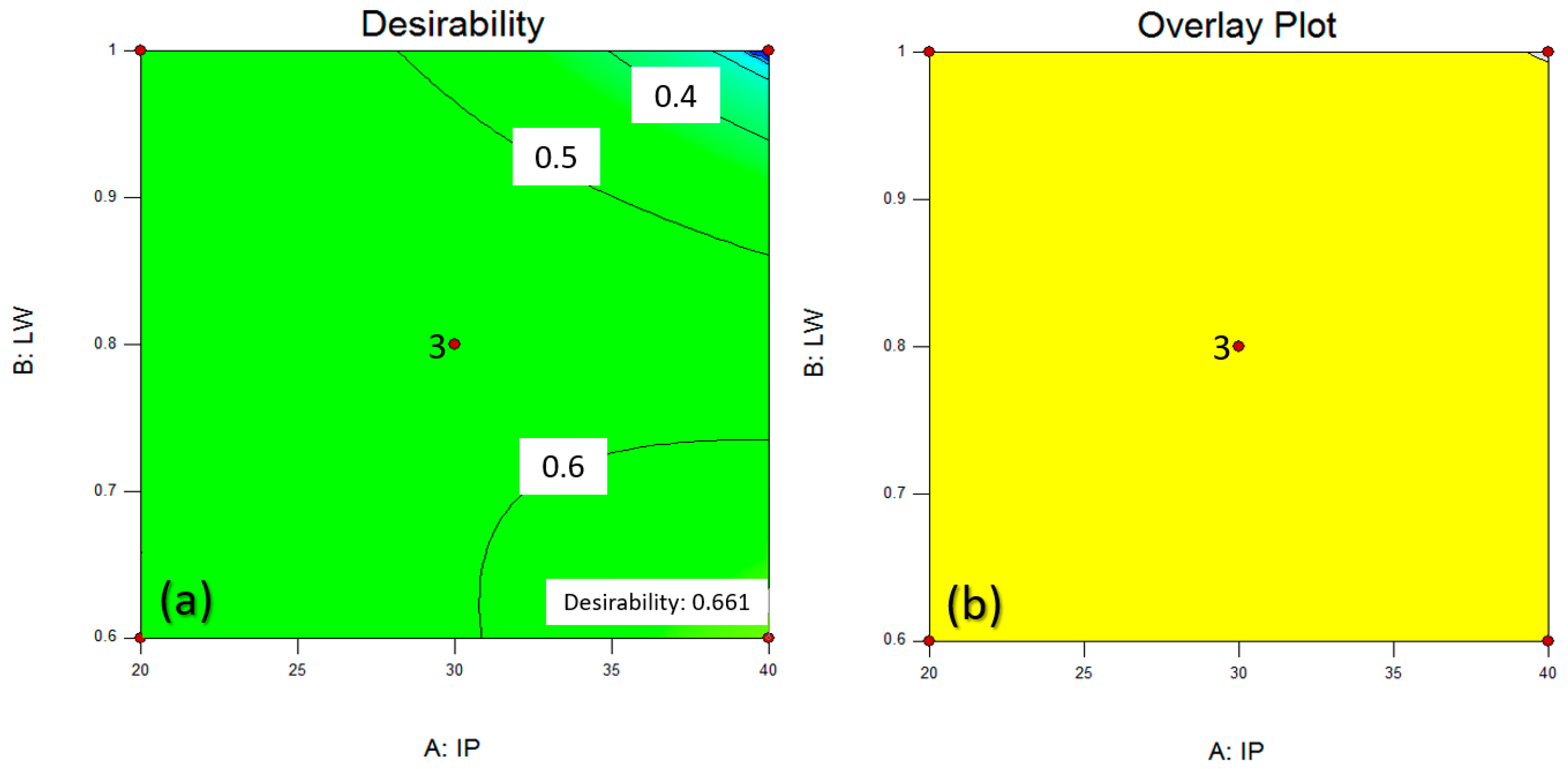
The ANOVA

Table 10. ANOVA for Response Surface 2FI model for Tensile strain at Yield.

Source	Sum of Squares	df	Mean Square	F-Value	p-Value
Model	7.663 × 10−6	3	2.554 × 10−6	2.70	0.1259
A-IP	5.296 × 10−7	1	5.296 × 10−7	0.56	0.4786
B-LW	5.693 × 10−6	1	5.693 × 10−6	6.02	0.0439
AB	1.440 × 10−6	1	1.440 × 10−6	1.52	0.2570
Residual	6.619 × 10−6	7	9.455 × 10−7
Lack of Fit	4.293 × 10−6	5	8.587 × 10−7	0.74	0.6611
Pure Error	2.325 × 10−6	2	1.163 × 10−6
Cor Total	1.428 × 10−5	10
			R-Squared = 53.66%		Adj R-Squared = 33.79%

for the Response Surface 2FI model provides insights into the significance of the model and its individual factors. The table displays the sums of squares, degrees of freedom, mean squares, F-values, and p-values for each source. In this case, the model as a whole does not show a significant effect on the response variable, as indicated by the p-value of 0.1259. This suggests that the 2FI model may not be a good fit for the data, and it does not explain a significant portion of the variation in the response variable [50]. Analyzing the individual factors, A-IP (infill percentages) and AB (interaction between infill percentages and layer width) do not show significant effects on the response variable, as indicated by their respective p-values of 0.4786 and 0.2570. This suggests that these factors may not have a significant impact on the response variable based on this model. However, the factor B-LW (layer width) does show a significant effect on the response variable, as indicated by its p-value of 0.0439. This suggests that layer width may have a significant impact on the response variable based on this model. The residual sum of squares represents the variation in the response variable that is not accounted for by the model. The lack of fit sum of squares compares the model’s fit to the replicated data. In this case, the lack of fit is not significant with a p-value of 0.6611. This indicates that the 2FI model adequately captures the variation in the data, and the remaining variation can be attributed to random error. The adj R-Squared value of 0.3379 indicates that the model explains approximately 33.79% of the total variation in the response variable. This suggests that the 2FI model has a moderate ability to explain the variation in the data.

Equation (6) provided relates the response variable (tensile strain at yield + 0.10) to the factors A-IP, B-LW, and their interaction term AB. The coefficients accompanying each factor indicate the magnitude and direction of their impact on the response variable. Positive coefficients suggest a positive effect on the response variable, while negative coefficients indicate a negative effect.

(Tensile strain at Yield + 0.10)³ = −1.10376 × 10⁻³ + 2.19006 × 10⁻⁴ × IP+5.55662 × 10⁻³ × LW − 3.00017 × 10⁻⁴ × IP × LW

(6)

Figure 11 presents a detailed analysis of the relationship between the input variables B:LW and A:IP and their impact on the response variable Tensile strain at Yield. The figure consists of both a contour plot (a) and a surface plot (b), providing insights into the relationship between the variables. The contour plot displays lines of equal Tensile strain at Yield, connecting regions with similar values of the response variable. By examining the contour lines, Tensile strain at Yield can be influenced by changes in B:LW and A:IP. From the contour plot, it is evident that increasing both B:LW and A:IP leads to a decrease in Tensile strain at Yield. The contour lines are more closely spaced and exhibit a downward trend as B:LW and A:IP values increase. This implies that higher values of B:LW and A:IP result in reduced Tensile strain at Yield.

The surface plot provides a three-dimensional representation of the relationship between B:LW, A:IP, and Tensile strain at Yield. It allows us to visualize the response variable as a function of the two input variables more comprehensively. The surface plot demonstrates a clear downward trend as B:LW and A:IP increase. As B:LW increases along the x-axis and A:IP increases along the y-axis, the surface plot reveals a decreasing pattern in Tensile strain at Yield. The surface becomes progressively lower as the values of B:LW and A:IP increase, indicating a reduction in Tensile strain at Yield.

4. Optimisation

The provided

Table 11. Constraints parameters for optimisation.

Name	Goal	Lower Limit	Upper Limit	Lower Weight	Upper Weight	Importance
A:IF (%)	is in range	20	40	1	1	3
B:LW (mm)	is in range	0.6	1	1	1	3
Weight (g)	minimize	7.25	10.09	1	1	3
Modulus (GPa)	maximize	1.08	1.43	1	1	3
Elongation Tensile Strength at Non-proportional Elongation (%)	maximize	0	6.94	1	1	3
Elongation at Break at Non-proportional Elongation (mm)	maximize	0	12.06	1	1	3
Tensile extension at Tensile Strength (mm)	maximize	−5.109	11.45	1	1	3
Tensile strain at Yield (mm/mm)	maximize	−0.01	0.06	1	1	3

presents the optimisation results for the previous parameters based on given constraints. Each row represents a different solution with specific values for the factors: IP (infill percentages), LW (layer width), Weight, Modulus, Elongation Tensile Strength at Non-proportional Elongation, Elongation at Break at Non-proportional Elongation, Tensile extension at Tensile Strength, and Tensile strain at Yield. The “Goal” column specifies the optimisation goal for each factor, whether it is to minimize or maximize its value. The “Limit” columns define the lower and upper limits within which each factor must fall. The “Weight” columns assign weights to each factor to reflect their relative importance in the optimisation process. The “Importance” column indicates the overall importance of each factor on a scale of 1 to 3. The “Desirability” column represents the desirability of each solution based on the optimisation criteria and constraints. The values range from 0 to 1, where higher values indicate more desirable solutions. The “Selected” label denotes the solution that has been chosen as the optimal solution based on the given criteria.

The “Desirability” column represents the desirability of each solution based on the optimisation criteria and constraints (

Table 12. Solutions obtained by constraints parameters.

Number	Input Parameters			Responses
	IP (%)	LW (mm)	Weight (g)	Modulus (GPa)	Elongation Tensile Strength at Non-Proportional Elongation (%)	Elongation at Break at Non-Proportional Elongation (mm)	Tensile Extension at Tensile Strength (mm)	Tensile Strain at Yield (mm/mm)	Desirability
1	40.000	0.600	8.514	1.21	4.835	10.320	8.960	0.055	0.662
2	39.738	0.600	8.499	1.21	4.835	10.273	8.945	0.055	0.661
3	40.000	0.607	8.511	1.21	4.792	10.144	8.876	0.054	0.660
4	20.000	0.951	7.881	1.21	2.866	8.207	6.429	0.040	0.571

). The values range from 0 to 1, where higher values indicate more desirable solutions. The “Selected” label denotes the solution that has been chosen as the optimal solution based on the given criteria.

Analyzing the solutions, Solution 1 is selected as the optimal solution with an infill percentage (IP) of 40, a layer width (LW) of 0.6, a weight of 8.514, a tensile extension at a tensile strength of 8.960, and a tensile strain at a yield of 0.055 (Figure 12).

5. Conclusions

Response Surface Methodology (RSM) effectively uncovers complex relationships between variables. It employs perturbation plots, surface plots, and Box-Cox plots to reveal variable sensitivity. This analysis identifies critical factors, optimizes material properties, and informs decisions for improved system performance. The study combines experimental data and statistical analysis to create predictive models for future optimisations and design enhancements. In summary, our findings lead to these conclusions:

• Higher infill percentages lead to increased modulus and stiffness, while thinner layer widths enhance tensile strength and rigidity.
• Response Surface Methodology (RSM) and Box-Cox transformation improved model accuracy and linearity.
• Elongation Tensile Strength at Non-proportional Elongation decreased with higher B-LW and lower A-IP.
• The layer width decreases and the infill percentage increases, the material’s ability to elongate before reaching the point of breakage decreases.
• Increasing B:LW and A:IP led to a reduction in the corresponding responses. This observation implies that higher values of layer width and infill percentage contribute to a decrease in the tensile extension at the point of tensile strength and the material’s strain at yield.
• Featuring a 40% infill percentage and 0.6 mm layer width, emerged as the optimal choice based on the given optimisation criteria and constraints. This particular combination of A:IP and B:LW resulted in a favourable balance of mechanical properties, including modulus, tensile strength, and elongation.

References

1. Mazzanti, V.; Malagutti, L.; Mollica, F. FDM 3D Printing of Polymers Containing Natural Fillers: A Review of their Mechanical Properties. Polymers 2019, 11, 1094. [Google Scholar] [CrossRef] [PubMed]
2. Cano-Vicent, A.; Tambuwala, M.M.; Hassan, S.S.; Barh, D.; Aljabali, A.A.A.; Birkett, M.; Arjunan, A.; Serrano-Aroca, Á. Fused deposition modelling: Current status, methodology, applications and future prospects. Addit. Manuf. 2021, 47, 102378. [Google Scholar] [CrossRef]
3. Ahmad, M.N.; Ishak, M.R.; Taha, M.M.; Mustapha, F.; Leman, Z. A Review of Natural Fiber-Based Filaments for 3D Printing: Filament Fabrication and Characterization. Materials 2023, 16, 4052. [Google Scholar] [CrossRef] [PubMed]
4. Radzuan, N.A.M.; Khalid, N.N.; Foudzi, F.M.; Royan, N.R.R.; Sulong, A.B. Mechanical Analysis of 3D Printed Polyamide Composites under Different Filler Loadings. Polymers 2023, 15, 1846. [Google Scholar] [CrossRef] [PubMed]
5. Ehrmann, G.; Ehrmann, A. Investigation of the Shape-Memory Properties of 3D Printed PLA Structures with Different Infills. Polymers 2021, 13, 164. [Google Scholar] [CrossRef]
6. Sandanamsamy, L.; Harun, W.S.W.; Ishak, I.; Romlay, F.R.M.; Kadirgama, K.; Ramasamy, D.; Idris, S.R.A.; Tsumori, F. A comprehensive review on fused deposition modelling of polylactic acid. In Progress in Additive Manufacturing; Springer: Berlin/Heidelberg, Germany, 2022. [Google Scholar] [CrossRef]
7. Lyu, Y.; Liu, D.; Guo, R.; Ji, Z.; Wang, X.; Shi, X. Flexibility of Diels-Alder reversible covalent bonds in fused deposition modeling 3D printing: Bonding and de-bonding. Polymer 2023, 266, 125637. [Google Scholar] [CrossRef]
8. Sharma, A.; Rai, A. Fused deposition modelling (FDM) based 3D & 4D Printing: A state of art review. Mater. Today Proc. 2022, 62, 367–372. [Google Scholar] [CrossRef]
9. Mishra, V.; Negi, S.; Kar, S. FDM-based additive manufacturing of recycled thermoplastics and associated composites. J. Mater. Cycles Waste Manag. 2023, 25, 758–784. [Google Scholar] [CrossRef]
10. Rajendran, S.; Palani, G.; Kanakaraj, A.; Shanmugam, V.; Veerasimman, A.; Gądek, S.; Korniejenko, K.; Marimuthu, U. Metal and Polymer Based Composites Manufactured Using Additive Manufacturing—A Brief Review. Polymers 2023, 15, 2564. [Google Scholar] [CrossRef] [PubMed]
11. Gibson, I.J.; Ashby, F. The mechanics of three-dimensional cellular materials. Proc. R. Soc. Lond. A Math. Phys. Sci. 1982, 382, 43–59. [Google Scholar] [CrossRef]
12. Kalita, S.J.; Bose, S.; Hosick, H.L.; Bandyopadhyay, A. Development of controlled porosity polymer-ceramic composite scaffolds via fused deposition modeling. Mater. Sci. Eng. C 2003, 23, 611–620. [Google Scholar] [CrossRef]
13. Drummer, D.; Cifuentes-Cuéllar, S.; Rietzel, D. Suitability of PLA/TCP for fused deposition modeling. Rapid Prototyp. J. 2012, 18, 500–507. [Google Scholar] [CrossRef]
14. Suzdaltsev, A.; Rakhmanova, O. Special Issue on Metal-Based Composite Materials: Preparation, Structure, Properties and Applications. Appl. Sci. 2023, 13, 4799. [Google Scholar] [CrossRef]
15. Mierzwiński, D.; Łach, M.; Gądek, S.; Lin, W.-T.; Tran, D.H.; Korniejenko, K. A brief overview of the use of additive manufacturing of con-create materials in construction. Acta Innov. 2023, 48, 22–37. [Google Scholar] [CrossRef]
16. Monaldo, E.; Ricci, M.; Marfia, S. Mechanical properties of 3D printed polylactic acid elements: Experimental and numerical insights. Mech. Mater. 2023, 177, 104551. [Google Scholar] [CrossRef]
17. Suteja, T.J.; Soesanti, A. Mechanical Properties of 3D Printed Polylactic Acid Product for Various Infill Design Parameters: A Review. J. Phys. Conf. Ser. 2020, 1569, 042010. [Google Scholar] [CrossRef]
18. Scaffaro, R.; Citarrella, M.C.; Gulino, E.F. Opuntia Ficus Indica based green composites for NPK fertilizer controlled release produced by compression molding and fused deposition modeling. Compos. Part A Appl. Sci. Manuf. 2022, 159, 107030. [Google Scholar] [CrossRef]
19. Turner, B.N.; Strong, R.; Gold, S.A. A review of melt extrusion additive manufacturing processes: I. Process design and modeling. Rapid Prototyp. J. 2014, 20, 192–204. [Google Scholar] [CrossRef]
20. Afsharkohan, M.S.; Dehrooyeh, S.; Sohrabian, M.; Vaseghi, M. Influence of processing parameters tuning and rheological characterization on improvement of mechanical properties and fabrication accuracy of 3D printed models. Rapid Prototyp. J. 2023, 29, 867–881. [Google Scholar] [CrossRef]
21. Nakajima, J.; Fayazbakhsh, K.; Teshima, Y. Experimental study on tensile properties of 3D printed flexible kirigami specimens. Addit. Manuf. 2020, 32, 101100. [Google Scholar] [CrossRef]
22. Wang, K.; Xie, X.; Wang, J.; Zhao, A.; Peng, Y.; Rao, Y. Effects of infill characteristics and strain rate on the deformation and failure properties of additively manufactured polyamide-based composite structures. Results Phys. 2020, 18, 103346. [Google Scholar] [CrossRef]
23. Moradi, M.; Karamimoghadam, M.; Meiabadi, S.; Casalino, G.; Ghaleeh, M.; Baby, B.; Ganapathi, H.; Jose, J.; Abdulla, M.S.; Tallon, P.; et al. Mathematical Modelling of Fused Deposition Modeling (FDM) 3D Printing of Poly Vinyl Alcohol Parts through Statistical Design of Experiments Approach. Mathematics 2023, 11, 3022. [Google Scholar] [CrossRef]
24. Rezayat, M.; Karamimoghadam, M.; Yazdi, M.S.; Moradi, M.; Bodaghi, M. Statistical analysis of experimental factors for synthesis of copper oxide and tin oxide for antibacterial applications. Int. J. Adv. Manuf. Technol. 2023, 127, 3017–3030. [Google Scholar] [CrossRef]
25. Heidari-Rarani, M.; Ezati, N.; Sadeghi, P.; Badrossamay, M. Optimization of FDM process parameters for tensile properties of polylactic acid specimens using Taguchi design of experiment method. J. Thermoplast. Compos. Mater. 2022, 35, 2435–2452. [Google Scholar] [CrossRef]
26. Jin, M.; Neuber, C.; Schmidt, H.-W. Tailoring polypropylene for extrusion-based additive manufacturing. Addit. Manuf. 2020, 33, 101101. [Google Scholar] [CrossRef]
27. Equbal, A.; Sood, A.K.; Equbal, M.I.; Badruddin, I.A.; Khan, Z.A. RSM based investigation of compressive properties of FDM fabricated part. CIRP J. Manuf. Sci. Technol. 2021, 35, 701–714. [Google Scholar] [CrossRef]
28. El Magri, A.; El Mabrouk, K.; Vaudreuil, S.; Touhami, M.E. Experimental investigation and optimization of printing parameters of 3D printed polyphenylene sulfide through response surface methodology. J. Appl. Polym. Sci. 2021, 138, 49625. [Google Scholar] [CrossRef]
29. Wickramasinghe, S.; Do, T.; Tran, P. FDM-Based 3D Printing of Polymer and Associated Composite: A Review on Mechanical Properties, Defects and Treatments. Polymers 2020, 12, 1529. [Google Scholar] [CrossRef]
30. Tanveer, M.Q.; Mishra, G.; Mishra, S.; Sharma, R. Effect of infill pattern and infill density on mechanical behaviour of FDM 3D printed Parts—A current review. Mater. Today Proc. 2022, 62, 100–108. [Google Scholar] [CrossRef]
31. Moradi, M.; Karamimoghadam, M.; Meiabadi, S.; Rasool, S.; Casalino, G.; Shamsborhan, M.; Sebastian, P.K.; Poulose, A.; Shaiju, A.; Rezayat, M. Optimizing Layer Thickness and Width for Fused Filament Fabrication of Polyvinyl Alcohol in Three-Dimensional Printing and Support Structures. Machines 2023, 11, 829–844. [Google Scholar] [CrossRef]
32. Patel, A.; Taufik, M. Extrusion-Based Technology in Additive Manufacturing: A Comprehensive Review. Arab. J. Sci. Eng. 2022, 140, 2044–2056. [Google Scholar] [CrossRef]
33. Krajangsawasdi, N.; Blok, L.G.; Hamerton, I.; Longana, M.L.; Woods, B.K.S.; Ivanov, D.S. Fused Deposition Modelling of Fibre Reinforced Polymer Composites: A Parametric Review. J. Compos. Sci. 2021, 5, 29. [Google Scholar] [CrossRef]
34. Moncayo-Matute, F.P.; Vázquez-Silva, E.; Peña-Tapia, P.G.; Torres-Jara, P.B.; Moya-Loaiza, D.P.; Viloria-Ávila, T.J. Finite Element Analysis of Patient-Specific 3D-Printed Cranial Implant Manufactured with PMMA and PEEK: A Mechanical Comparative Study. Polymers 2023, 15, 3620. [Google Scholar] [CrossRef] [PubMed]
35. Chalgham, A.; Ehrmann, A.; Wickenkamp, I. Mechanical Properties of FDM Printed PLA Parts before and after Thermal Treatment. Polymers 2021, 13, 1239. [Google Scholar] [CrossRef]
36. Portoacă, A.I.; Ripeanu, R.G.; Dini, A.; Tănase, M. Optimization of 3D Printing Parameters for Enhanced Surface Quality and Wear Resistance. Polymers 2023, 15, 3419. [Google Scholar] [CrossRef]
37. Pepelnjak, T.; Stojšić, J.; Sevšek, L.; Movrin, D.; Milutinović, M. Influence of Process Parameters on the Characteristics of Additively Manufactured Parts Made from Advanced Biopolymers. Polymers 2023, 15, 716. [Google Scholar] [CrossRef]
38. Susmel, L.; Berto, F.; Hu, Z. The Strain energy density to estimate lifetime of notched components subjected to variable amplitude fatigue loading. Frat. Integrità Strutt. 2018, 13, 383–393. [Google Scholar] [CrossRef]
39. Pertuz-Comas, A.D.; Díaz, J.G.; Meneses-Duran, O.J.; Niño-Álvarez, N.Y.; León-Becerra, J. Flexural Fatigue in a Polymer Matrix Composite Material Reinforced with Continuous Kevlar Fibers Fabricated by Additive Manufacturing. Polymers 2022, 14, 3586. [Google Scholar] [CrossRef]
40. Rezayat, M.; Moradi, M.; Mateo, A. Nanosecond pulsed laser surface processing of AISI 301LN steel: Effect on surface topography and mechanical properties. Int. J. Adv. Manuf. Technol. 2023, 128, 3025–3040. [Google Scholar] [CrossRef]
41. Raj, S.A.; Muthukumaran, E.; Jayakrishna, K. A Case Study of 3D Printed PLA and Its Mechanical Properties. Mater. Today Proc. 2018, 5, 11219–11226. [Google Scholar] [CrossRef]
42. Travieso-Rodriguez, J.A.; Jerez-Mesa, R.; Llumà, J.; Traver-Ramos, O.; Gomez-Gras, G.; Rovira, J.J.R. Mechanical Properties of 3D-Printing Polylactic Acid Parts subjected to Bending Stress and Fatigue Testing. Materials 2019, 12, 3859. [Google Scholar] [CrossRef] [PubMed]
43. ASTM Standards, Standard Test Method for Tensile Properties of Plastics, ASTM International, PA, USA. 2012. Available online: https://www.astm.org/d0638-03.html (accessed on 21 August 2023).
44. Woigk, W.; Fuentes, C.A.; Rion, J.; Hegemann, D.; van Vuure, A.W.; Dransfeld, C.; Masania, K. Interface properties and their effect on the mechanical performance of flax fibre thermoplastic composites. Compos. Part A Appl. Sci. Manuf. 2019, 122, 8–17. [Google Scholar] [CrossRef]
45. Nelson, K.; Kelly, C.N.; Gall, K. Effect of stress state on the mechanical behavior of 3D printed porous Ti6Al4V scaffolds produced by laser powder bed fusion. Mater. Sci. Eng. B 2022, 286, 116013. [Google Scholar] [CrossRef]
46. Shanmugam, V.; Rajendran, D.J.J.; Babu, K.; Rajendran, S.; Veerasimman, A.; Marimuthu, U.; Singh, S.; Das, O.; Neisiany, R.E.; Hedenqvist, M.S.; et al. The mechanical testing and performance analysis of polymer-fibre composites prepared through the additive manufacturing. Polym. Test 2021, 93, 106925. [Google Scholar] [CrossRef]
47. Vamshinath, K.; Kumar, N.N.; Kumar, R.T.; Nagaraju, D.S.; Sateesh, N.; Subbaiah, R. Analysis of the effect of the process parameters on the mechanical strength of 3D printed and adhesively bonded PETG single lap joint. Mater. Today Proc. 2022, 62, 4509–4514. [Google Scholar] [CrossRef]
48. Dutra, T.A.; Ferreira, R.T.L.; Resende, H.B.; Blinzler, B.J.; Larsson, R. Expanding Puck and Schürmann Inter Fiber Fracture Criterion for Fiber Reinforced Thermoplastic 3D-Printed Composite Materials. Materials 2020, 13, 1653. [Google Scholar] [CrossRef]
49. Sheoran, A.J.; Kumar, H. Fused Deposition modeling process parameters optimization and effect on mechanical properties and part quality: Review and reflection on present research. Mater. Today Proc. 2020, 21, 1659–1672. [Google Scholar] [CrossRef]
50. Melenka, G.W.; Cheung, B.K.O.; Schofield, J.S.; Dawson, M.R.; Carey, J.P. Evaluation and prediction of the tensile properties of continuous fiber-reinforced 3D printed structures. Compos. Struct. 2016, 153, 866–875. [Google Scholar] [CrossRef]
Figure 1. Flow chart of the 3D printing process [29].
Machines 11 00950 g001
Figure 2. Schematic of the (a) 3D printing process, (b) dimension of the layer.
Machines 11 00950 g002
Figure 3. Schematic of geometrical dimensions of the tensile test sample according to ASTM D638 2003.
Machines 11 00950 g003
Figure 4. (a) The 3D printed specimens, (b) fractured specimens after tensile test.
Machines 11 00950 g004
Figure 5. (a) specimen 1 with high elongation, (b) specimen 3 with high modulus (Note: triangle sign (▲) shows the maximum of the load).
Machines 11 00950 g005
Figure 6. Relationship between A and B as input variables on the responses; (a) perturbation plot and (b) normal plot of residuals. (colored squares are distributions of the data from the trend line and the middle red circle represents the mean of normal data).
Machines 11 00950 g006
Figure 7. Box-Cox plot for the relationship between A and B as input variables on the responses; (a) perturbation plot and (b) box-cox plot.
Machines 11 00950 g007
Figure 8. (a) Box-Cox and (b) surface plot for Elongation Tensile Strength at Non-proportional Elongation.
Machines 11 00950 g008
Figure 9. (a) Perturbation and (b) surface plot for Elongation at Break at Non-proportional Elongation.
Machines 11 00950 g009
Figure 10. (a) contour, (b) surface plot for Tensile extension at Tensile Strength.
Machines 11 00950 g010
Figure 11. (a) Contour and (b) surface plot for Tensile strain at Yield.
Machines 11 00950 g011
Figure 12. (a) Desirability and (b) overlay plot for an optimal solution.
Machines 11 00950 g012