
Kinematic Modelling of a 3RRR Planar Parallel Robot Using Genetic Algorithms and Neural Networks


Centro de Automática y Robótica (UPM-CSIC), Universidad Politécnica de Madrid-Consejo Superior de Investigaciones Científicas, José Gutiérrez Abascal 2, 28006 Madrid, Spain
*
Author to whom correspondence should be addressed.
Machines 2023, 11(10), 952; https://doi.org/10.3390/machines11100952
Submission received: 21 September 2023
/
Revised: 5 October 2023
/
Accepted: 10 October 2023
/
Published: 12 October 2023
(This article belongs to the Section Machine Design and Theory)
Abstract
:Kinematic modelling of parallel manipulators poses significant challenges due to the absence of analytical solutions for the Forward Kinematics (FK) problem. This study centres on a specific parallel planar robot, specifically a 3RRR configuration, and addresses the FK problem through two distinct methodologies: Genetic Algorithms (GA) and Neural Networks (NN). Utilising the Inverse Kinematic (IK) model, which is readily obtainable, both GA and NN techniques are implemented without the need for closed-loop formulations or non-systematic mathematical tools, allowing for easy extension to other robot types. A comparative analysis against an existing numerical method demonstrates that the proposed methodologies yield comparable or superior performance in terms of accuracy and time, all while reducing development costs. Despite GA’s time consumption limitations, it excels in path planning, whereas NN delivers precise results unaffected by stochastic elements. These results underscore the feasibility of using neural networks and genetic algorithms as viable alternatives for real-time kinematic modelling of robots when closed-form solutions are unavailable.
1. Introduction
A parallel manipulator is a “closed-loop kinematic chain mechanism whose terminal element can be linked to its base by means of different kinematic chains arranged in parallel” [1]. Within these mechanisms, it is possible to reach the terminal element (or any other point on it) from the base, where the actuators are typically located, by traversing various paths, in contrast to serial robots where the path between the base and the end is distinctly defined.
The advantages of parallel manipulators include load distribution among all arms, high speed and acceleration, enhanced precision, and reduced weight compared to serial robots [2,3]. However, they tend to have a smaller workspace and more complex kinematic equations, making control more challenging [4,5,6]. An illustrative example is the Stewart platform [7], whose Forward Kinematic (FK) model can yield up to 40 solutions, which, to this day, remains computationally infeasible for real-time numerical computation [8].
As a result, their applications are typically centred on tasks such as pick and place operations [9], supporting heavy loads, cutting [10], high-precision activities like painting [11], or in recreational and virtual reality simulation applications [12]. Variants of the aforementioned Stewart platform are commonly employed in these applications.
Within the domain of parallel robots, there exists a dedicated line of research focused on planar mechanisms, which possess only three degrees of freedom. One example is the 3RRR robot, a manipulator consisting of three kinematic chains, each with three rotating joints, which will be introduced in Section 2.1. This research area initially emerged during the 1990s from a purely mechanical perspective [4,13,14]; however, it was not until recent years that it attracted the attention of researchers in the area of robotics, with a main focus on solving dynamic aspects [15,16,17], analysing its singularities [18], and optimising its workspace [19,20,21,22].
Their interest, beyond possible applications such as welding [17], working with heavy weights, and aiding gait rehabilitation tasks [23,24], is the inherent complexity. Almost all the challenges of parallel robots, including singularities, multiple solutions, and the impossibility of obtaining the FK and differential models in an analytical way, are present in them. Consequently, they have become research tools, with authors trying to find in them efficient techniques that can be extrapolated to other less-demanding robot typologies.
In particular, this work focuses on Forward Kinematic (FK) modelling. While the Inverse Kinematic (IK) model, which involves determining the actuator angles based on the robot end-effector’s position and orientation, can be derived analytically using geometric reasoning, FK modelling invariably necessitates numerical and/or Artificial Intelligence (AI) methods.
Indeed, ref. [13] showed that the treatment of the global equations of the robot in order to obtain x, y, and orientation () from the motor angles leads, in the general case, to a sixth-order polynomial. Analytic (or lower-degree polynomial) solutions are only achievable in certain simple scenarios, such as those described in [25], which reduces the central platform to a single bar, [13] in which the triangle becomes a segment and the base becomes arranged on a line parallel to it, or [14] in which the triangle of the platform is similar to the one of the base.
In all other situations, it is necessary to have recourse to numerical minimisation methods, as is done in [26,27]. Other authors have proposed to approach the problem with a search on manifolds [28], constraint curves [29], or simplifying the equations by including as input the value of the passive angles, which were previously determined [30].
Genetic Algorithms (GA) and Neural Networks (NN) have been successfully employed for other robotic structures ([31,32,33,34] provides examples for GA, [35,36,37,38,39] for NN, and [40] for a work in which both methodologies are used and compared) but never for 3RRR robots and, as has been shown, they avoid the problem of singularities [40] and can be used for path following [33,39].
The aim of this work was to solve the FK problem from AI tools, partially or totally blind to the physical characteristics of the mechanism. The paper presents two primary contributions. Firstly, a GA was developed employing the IK model as the fitness function. In contrast to existing numerical methods, this approach avoids the need for closed-loop formulations or other mathematical tools that lack geometric intuition and systematicity, particularly in the case of planar parallel robots. Additionally, this method is entirely indifferent to the presence of singular points and performs well even in their vicinity, which is particularly valuable when, as will be explained when describing the robot, singularities are abundant and unavoidable.
Secondly, a feedforward NN was trained using data generated from the IK model. Once the training process was completed, the NN was able to predict the final position and orientation, given the input actuator angles. Although the data used for training were obtained through simulation, they could be sourced from a real robot, making the solution theoretically independent of any kinematic model of the robot. Moreover, the influence of singularities was limited within this methodology.
This paper is structured as it follows: Section 2 introduces the IK model of the parallel planar manipulator and presents a numerical model, based on [26], which was used to compare the validity of the AI-based solutions. These techniques, which constitute the main contribution of this work, are detailed in Section 3. Section 4 presents the results and, subsequently, Section 5 compares them, highlighting the advantages and disadvantages of each methodology. Finally, Section 6 draws the conclusion.
2. The 3RRR Planar Parallel Robot: Kinematic Analysis
2.1. Geometric Description
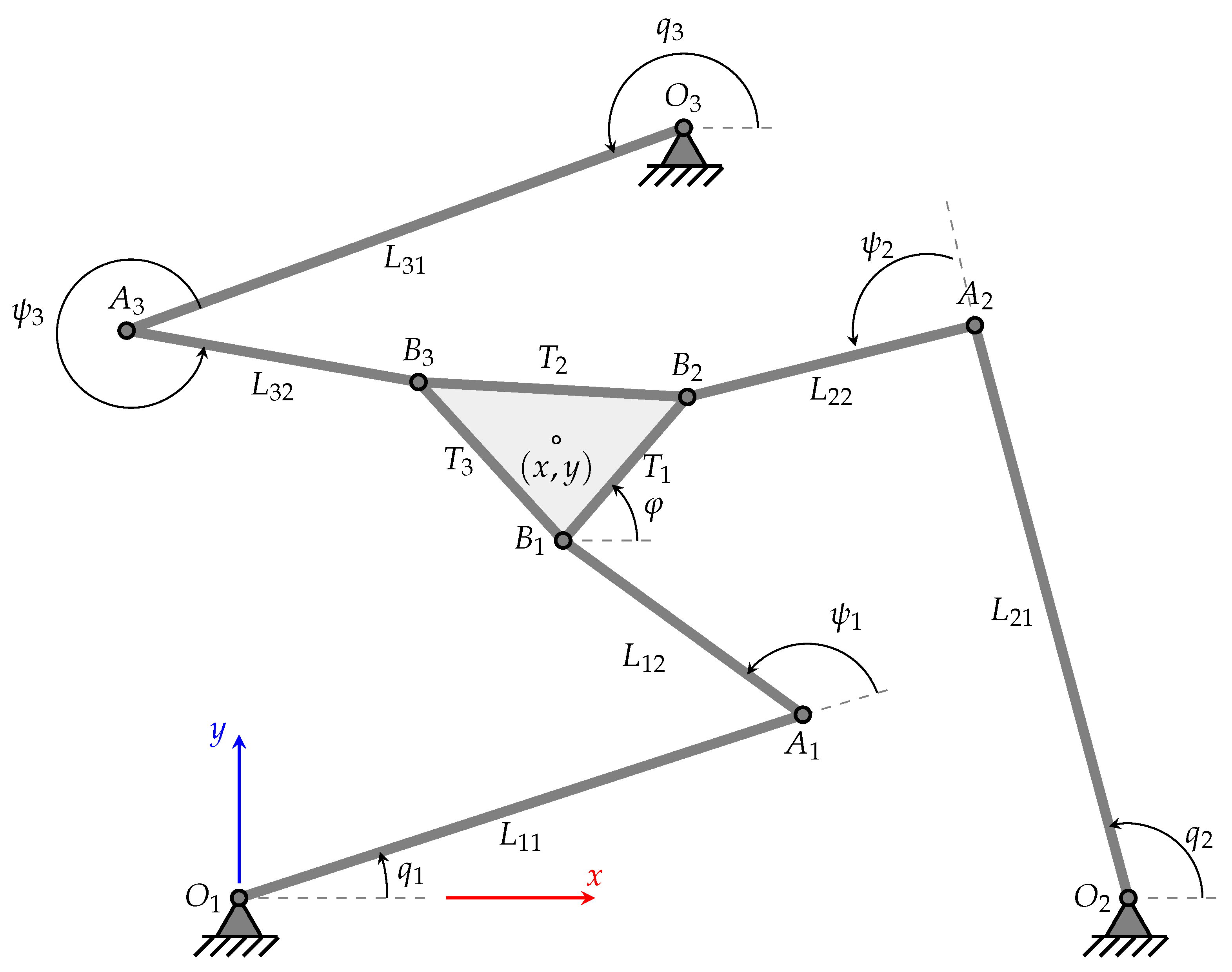
The 3RRR robot, shown in Figure 1, is a parallel planar robot with three rotating degrees of freedom. Its centre is a triangular platform (not necessarily equilateral) connected to its three bases —where the actuators are located—by means of three kinematic chains. Each of them consists of two rods linked by a rotating joint.
The usual reference system is a Cartesian axis located in the base . There is no unique nomenclature in the literature. In the framework of the present work, the nomenclature specified in Table 1 is followed. Specifically, the variable describing the position of the centre point of the platform and the orientation of the platform is referred to as and refers to the actuator angles, measured counter-clockwise and taking the x-axis as the origin. The passive angles (those of the joints) are denoted as .
2.2. Singularities
A common problem related to parallel planar robots is that of singularities: configurations in which the degrees of freedom are reduced or increased, causing the behaviour to become unpredictable. At these points, no movement is appreciated in when varies, or vice versa. This can be considered one of the major drawbacks of robots of this type, as they reduce an already generally small working space.
Three types of singularities can appear [41,42]. On the one hand, indirect singularities (or type I singularities) occur at points where the robot, as a consequence of having one kinematic chain totally enlarged, loses one degree of freedom. These singularities tend to appear in the boundaries of the workspace and are analogous, from a geometrical point of view, to the ones that are present in serial robots.
On the other, direct singularities (or type II singularities) occur at positions where, with its actuators fully locked, the robot central platform (or equivalent end part of the mechanism) is locally mobile, which means that the manipulator is gaining, at these points, one or more degrees of freedom.
These singularities have been widely studied from a dynamical point of view [43] because if the links are not able to resist forces or torques when the actuators are blocked, the robot can become damaged. In addition, they tend to appear in the centre of the workspace, so, if a distant point needs to be reached, it is practically obligatory to pass through them. However, even from a purely kinematic point of view, they are of interest, which is why they are dealt with in this article. This is because, due to the continuous nature of a robot’s workspace [44], even near to it, big changes in are produced with only little movements in the articular coordinates .
Finally, type III singularities are positions where both previous singularities are present at the same time. These degenerated situations are very strange and only appear if some conditions on the linkage parameters are satisfied [41].
2.3. Inverse Kinematic Modelling
The IK model obtains the values of the angles of the actuators from the position and orientation of the platform . As [20] demonstrates, the general case has eight possible solutions, depending on the arrangement of the passive angles.
The usual way to approach the problem is to start by obtaining the coordinates of the vertices of the triangle and from there, solve each kinematic chain separately. It is common, for convenience, to impose restrictions on the values of the lengths of the kinematic chains or on the position of the bases [20,21,23] in order to simplify the equations.
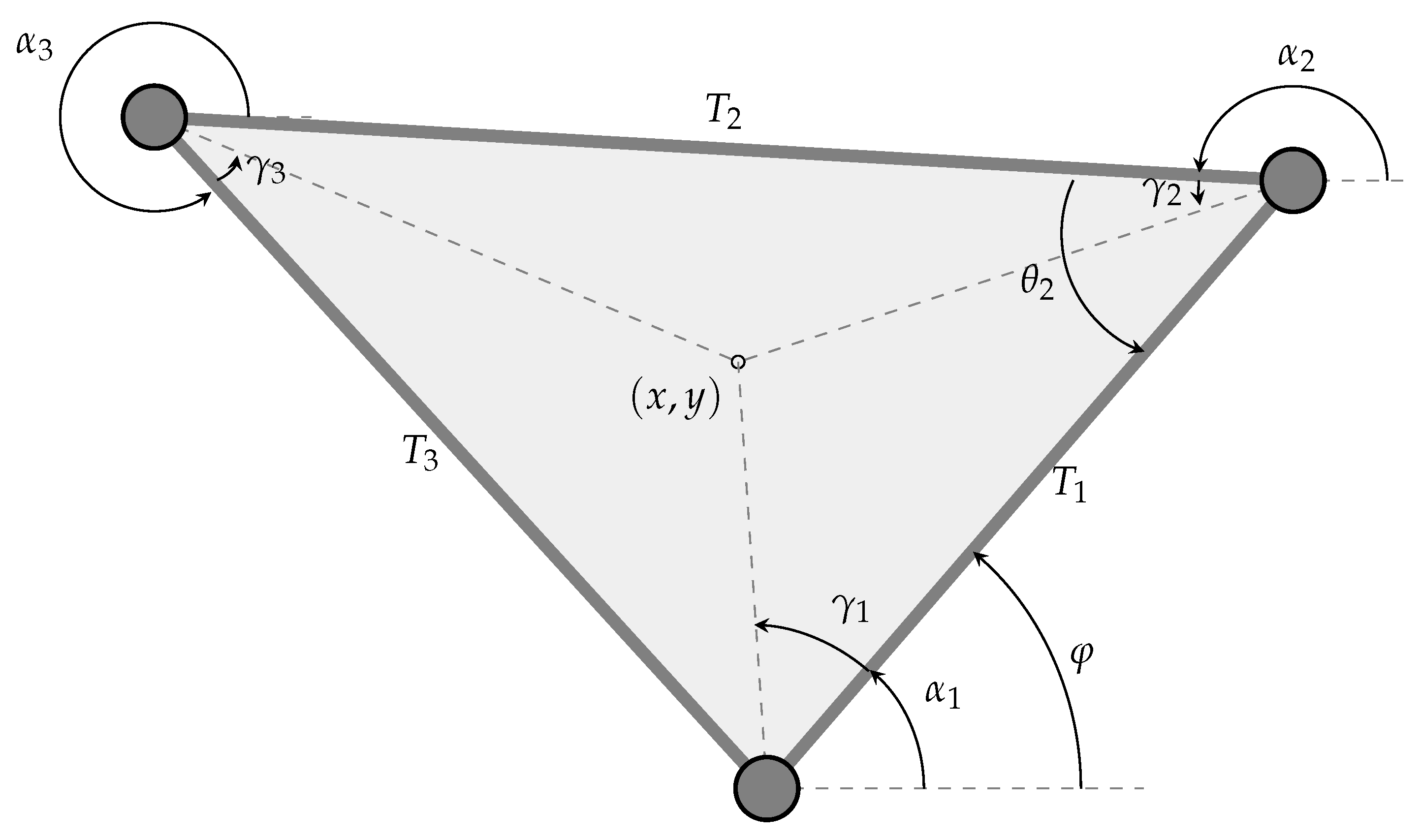
Because in this work a robot with the most general configuration possible is desired, a method capable of admitting any asymmetry was developed. Unlike [45], which also starts from this premise, the lengths of the sides of the triangle, and not the medians, are taken as known variables, as they are considered a much more natural magnitude.
To do this, the angles that the sides of the triangle form with respect to the reference axis are obtained from the parameters drawn in Figure 2. The first step is to calculate, with the law of cosines, the internal angles of the triangle:
From them, platform vertices are expressed in the local axes shown in Figure 2, making it possible to directly calculate the lengths of the half medians.
With them, angles are obtained:
which make possible to calculate the values of the angles:
From there, it is possible to immediately obtain :
Each kinematic chain is now defined by a system of two non-linear equations with two variables ( and ):
where
This equation can be rewritten as:
where
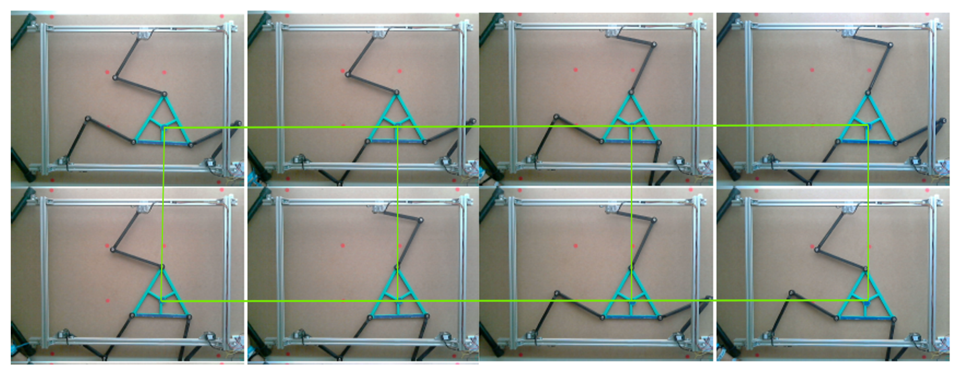
Equation (14) reaches two real solutions in the general case, when . Because each kinematic chain is completely independent, either of the two solutions can be chosen for this solution, independently of the choice of the other two , which results in the eight possible configurations previously mentioned, which can be seen in Figure 3. If only one solution is obtained, i.e., if , the robot is in an inverse singularity, where some degrees of freedom are lost. Complex solutions refer to points outside the robot’s workspace. There is no possibility to easily identify direct singularities using Equation (14) as they are related to FKs.
2.4. FK Modelling—Numerical Method
As mentioned above, it is impossible to obtain an analytical expression from which to calculate when is known. Up to six solutions can be attained [4]. A method of approaching inverse modelling based on [26] is presented here and was used as a basis for comparison against the implemented AI algorithms.
Starting from the closed loop:
Equations are squared and summed:
Because the previous expression is valid for the three kinematic chains, it can be expressed as a system of three non-linear equations with three unknowns :
To solve it, the Newton–Raphson method is used:
where is the matrix with the derivatives of , which is different from robots’ Jacobian matrix, with the expression:
The algorithm stops if one of these conditions is met:
- If the difference between two consecutive solutions, and , measured in norm 2, is less than a value tol1, previously set;
- A total of 100 iterations have been completed.
If case one occurs, the algorithm is considered to have converged. In the same way, convergence is reached if, after the 100 iterations, the distance between and is smaller than tol2. Obviously, it is then necessary for tol1< tol2.
In this work, the values of tol1 and tol2 were set to 0.1 mm and 1 mm, respectively. That does not mean that a precision of 1 mm is ensured, but that the algorithm stops when, between two successive calculations, the final results of differ by less than that amount. Nothing guarantees that the returned is the correct value, but if it is located near , the Newton–Raphson method ensures convergence in the majority of cases.
Despite this methodology offering good results in terms of precision and speed, especially when following paths [26], it presents two major disadvantages. First of all, because the relation between and is established, convergence problems may arise near to singular points. As introduced in Section 2.2, direct singularities are points where platform’s position, , evolves fast with little changes in the articular coordinates, . This means that, near singularities, quotient is high and, in consequence, will be very different from .
Given that these points are located in the centre of the robot’s workspace, they cannot be easily avoided when making paths. However, solutions have been proposed to mitigate these issues. One approach involves locally characterising the singularity-free C-space, as done in [28], which is complete from an algorithmic point of view but very expensive. Another idea, presented in [46], focuses on moving at each step, minimising the risk of falling into singularities.
Secondly, the non-intuitive mathematical formulation required here is difficult to adapt for other planar parallel robots. Solutions, such as the ones presented in [47,48,49,50] for different structures, are very different from each other and involve considerable difficulty.
In contrast to serial robotics, where obtaining the FK model can be straightforward using the Denavit–Hartenberg method, it is the IK model that can be systematically derived in parallel robotics. While some authors have attempted to establish a unified methodology for obtaining the FK model of parallel planar robots [51,52], their findings tend to be intricate and only applicable to a limited set of structures.
These two drawbacks are solved using the two methodologies implemented in this work.
3. Fk Modelling Using AI Techniques
3.1. Genetic Algorithms Approach
In this section, the proposed genetic algorithm is described. Its main benefit is that it allows the FK model to be solved from the known, analytical IK equations alone, without the need for additional geometric relations and their derivatives.
Algorithm individuals are defined using six genes: three of them are responsible for establishing the position and orientation of the robots’ end-effector and three of them for defining which of the eight possible solutions of the IK model will be chosen—one for defining each in Equation (14).
Because the response is expected almost immediately, the algorithm parameters had to be configured to achieve both a good accuracy and speed of execution. The most critical part was the selection phase, which requires the execution of the IK model of each individual in each generation. In order to achieve a correct adjustment, nearly 900 simulations were carried out, varying the algorithm configuration parameters, which are presented in Table 2, and some of the algorithm’s criteria (distance measurement, existence of migration, etc.). Based on this information, the following sections justify the different methods used and some of the decisions taken. The complete algorithm can be found in Algorithm 1.
| Algorithm 1: Complete Genetic Algorithm | |||||||
| Function GeneticMCD() is | |||||||
| Initialise parameters with the values shown in Table 2 | |||||||
| for to do | |||||||
| for to do | |||||||
| calculate MCI of | |||||||
| end | |||||||
| Sort descending according to the values of | |||||||
| if then | |||||||
| Algorithm has converged | |||||||
| return | |||||||
| end | |||||||
| for to do | |||||||
| Two random robots from | |||||||
| robots(robot) ← Crossover(r1, r2) | |||||||
| robots(robot) ← Mutate() | |||||||
| end | |||||||
| if robots(1).fitness < tolG2 then | |||||||
| Algorithm has converged | |||||||
| return robots(1).P | |||||||
| else | |||||||
| Algorithm has not converged | |||||||
| return Error | |||||||
| end | |||||||
| end | |||||||
| end | |||||||
3.1.1. Generation
In the first phase, NRobots individuals are generated, assigning to its genes values following a normal distribution , with the mean of the current coordinates of the robot and standard deviation . The value of S is given by the expression:
where denotes the vector going from to .
Equation (20) corresponds to the area of the triangle formed by the actuators of the robot. Although the robot workspace can exceed or be enclosed within this triangle, it can be considered a good approximation of the size of the workspace without much calculation required.
The aim of using such a distribution is to generate points in the vicinity of the point where the robot is located (which seems natural when following trajectories), defining the vicinity in a way that can be adapted to different robot sizes. Moreover, the use of a normal distribution, whose domain is non-bounded, allows to generate a point in the whole workspace of the robot.
For every individual generated, the IK model is calculated. If it is located outside robot workspace—if, at least, one of its , calculated using Equation (14), takes complex values—it is discarded and regenerated.
The experiments showed that, although this methodology offered good results in the vast majority of the cases, it took a long time to generate valid individuals in the boundaries of the workspace, because individuals located in the vicinity were very likely to be non-valid. In addition, it was not easy to classify a priori if a point was near the boundaries or not. To solve the problem, when the number of discarded individuals reached , the point was considered a borderline point and the generation process changed. The values of for the subsequent individuals were then randomly taken from the intervals presented in Table 3.
In both of the methodologies, the individual is also composed of three other genes that indicate, for each kinematic chain, the sign in Equation (14). The generation algorithm is presented in Algorithm 2.
| Algorithm 2: Generation Algorithm | |||||||
| Function GenerateIndividuals() is | |||||||
| Robot current position | |||||||
| for to do | |||||||
| new 3RRR Robot | |||||||
| if then | |||||||
| Three values chosen following | |||||||
| else | |||||||
| Three values chosen following an Uniform Distribution with the intervals presented in Table 3. | |||||||
| end | |||||||
| Three values randomly taken from the set | |||||||
| Calculate MCI | |||||||
| if some of the values of is not real then | |||||||
| continue | |||||||
| end | |||||||
| end | |||||||
| return robots | |||||||
| end | |||||||
3.1.2. Fitness Evaluation
For each individual, its IK model was calculated, taking into account the considerations discussed in the previous paragraph, obtaining, in consequence, a vector with the angles of the actuators. The fitness function compares that value with the desired combination of actuators, , using the following formula:
Although initially, the 2-norm was considered, it was noted that very significant errors could be made if two angles are very close to the desired angles but one is at a certain distance. The use of the infinity norm, on the other hand, makes it possible to ensure that all are as close as desired.
3.1.3. Selection
In order to reach efficient results, a method with high selective pressure was selected in this step. Although in a first phase, Boltzmann selection was used, the difficulties in setting the parameters of the formula correctly made it preferable to opt for a straightforward sorting. The small number of individuals did not, moreover, make it too time-consuming.
The percentage of the individuals specified in PParents was selected, in each generation, as parents. This value was determined experimentally, taking the point in which the average error at the end of the algorithm reached a minimum value. Too few parents result in too little diversity, which stagnates the algorithm, while too many parents give good individuals little chance to reproduce.
3.1.4. Crossover
For the three first genes, containing the values of each individual, the average crossover was taken. This could not be implemented for the rest of the individual, in which binary crossover, with one cut-off point, was selected. No crossover probability was considered necessary due to the high selective pressure of the previous step. A pseudo-code implementation is detailed in Algorithm 3.
| Algorithm 3: Crossover Algorithm |
 |
3.1.5. Mutation, Migration, and Elitism
Highest mutation rates give more probability to reach a good solution early, but also give a higher number of incorrect solutions. In order to balance both aspects, elitism was implemented carrying all of the parents to the following generation and mutation was only applied to the individuals generated in the crossover step.
A mutation probability of MutPr was set. The mutation operation consists in multiplying each individual’s values by a number taken randomly taken from the interval following a uniform distribution. In comparison to directly summing a random value, this solution gave better results and does not need scaling values for the component. The implemented solution is presented in Algorithm 4.
The migration operator was initially implemented, generating random individuals at some steps of the process, but no better results were achieved and, in consequence, it was discarded.
| Algorithm 4: Mutation Algorithm |
 |
3.1.6. Stopping Criteria
The algorithm stops if one of these conditions is met:
- If, after the selection step, at least one individual’s objective function is below an error threshold tolG1;
- MaxGen generations have been completed.
If case one occurs, the algorithm is considered to have converged. In the same way, convergence is reached if, after the 100 iterations, the fitness of the best individual is less than tolG2. As happened in the numerical method, tolG1 must be greater than tolG2.
In this case, values for tolG1 and tolG2 were set to 0.29 (typical encoder resolution) and 1. The results are analysed in Section 4 and compared with those achieved by the numerical method and the neural network.
3.2. Neural Networks Approach
As a second technique for modelling the forward kinematics of the 3RRR robot, a neural network was used. The net was trained using simulation values given by the IK model, although it can be trained using data from a real robot, which makes the method totally agnostic to the modelling challenges of planar manipulators. Three parameters are expected at the input: the desired values of ; and at the output, corresponding values must be returned.
3.2.1. Network Setup
To manage redundancy, eight feedforward neural networks were used to solve this task. All of them have an identical structure and only differ in their training data. Each was trained with only a combination of the signs in Equation (14), i.e., with the data coming from only one of the solutions of the IK model. A redundancy-avoidance process, which will be presented in Section 3.2.3, was implemented to choose between the solutions provided by the eight networks.
Each net consists of two layers: a first layer of 25 neurons and the output layer of 3. Their sizes were adjusted experimentally, trying to keep the size as small as possible (more neurons mean more training time) but looking for acceptable errors.
A tansig function, with expression , was chosen as the activation function for the hidden layer, because it outperformed the results offered by a sigmoid, which caused training to stall. For the output layer, a pure lineal layer was chosen due to its capacity to deal with both positive and negative values, unlike what happens when using a ReLU layer. The Levenberg–Marquardt algorithm was selected as the training function. No bigg differences were observed between the different tested functions (Levenberg–Marquard, BFGS quasy-Newton, and conjugate gradients), so the Matlab default option was kept.
As the performance criterion, Mean Squared Error (MSE) was used. This is the most common option when working with neural networks for regression tasks. In this case, moreover, the MSE measures the Euclidean distance between the solution predicted by the network, , and the real one, , which seems the most natural alternative. It is true that has units other than x andy. However, normalising the data to the interval erases these differences.
3.2.2. Network Training
Each network was trained with data generated using the IK model. A total of 300,000 points were used for each one: 70% of them for the training process, 15% for validation, and 15% for testing. Although this number can be considered excessive for the size of the workspace (details of the robots used in the experiments are presented in Section 3.3), the high number of singularities associated to these manipulators make it necessary to work with a high number of points.
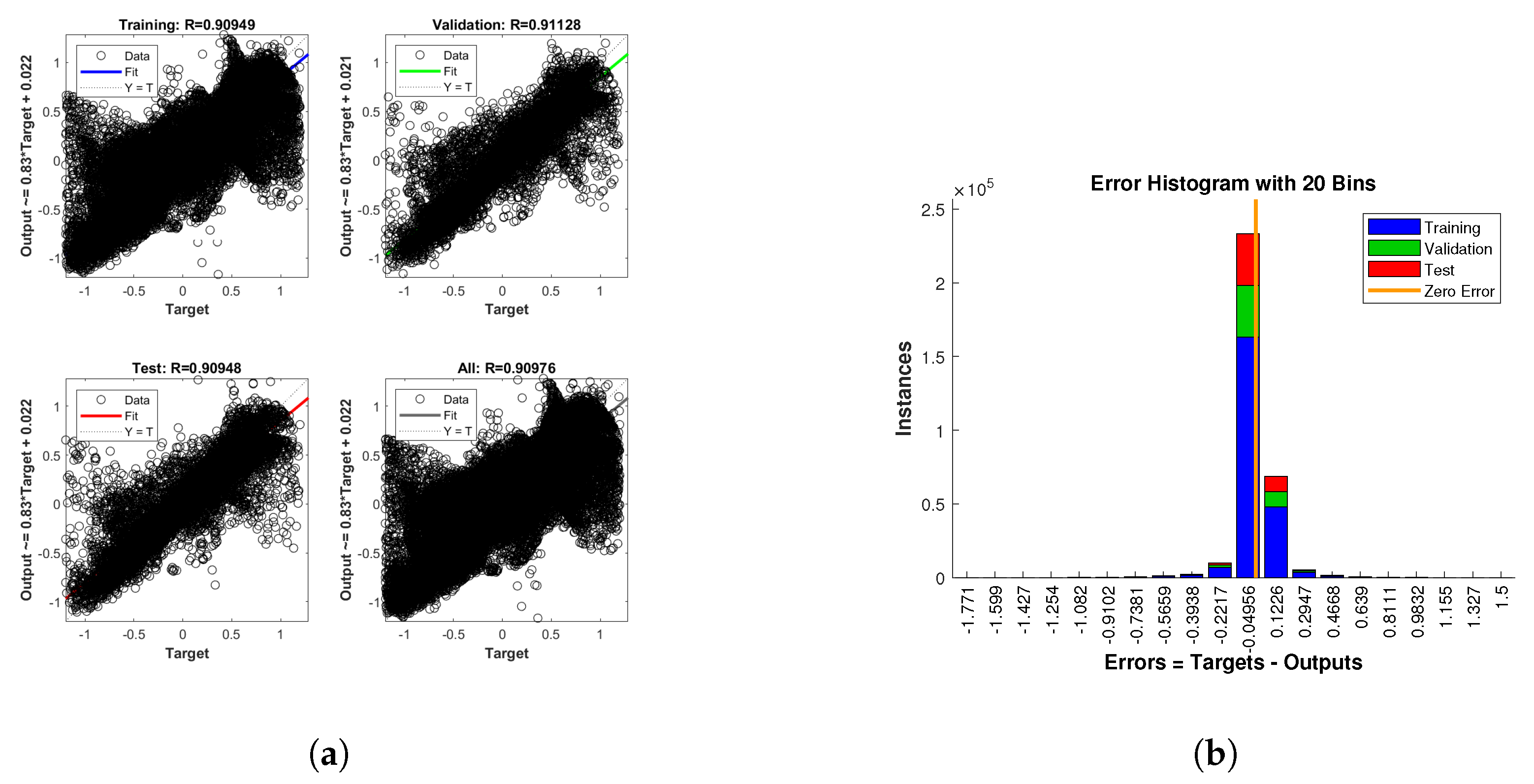
Training concluded after 1000 epochs or when the average error of the test data increased during the last 10 generations. This last criterion was implemented to avoid overfitting and was, in almost all of the training sessions carried out on the net, the limiting criterion. Matlab Deep Learning Toolbox was used for the training process. Usually, it finished after a number of iterations between 400 and 600 and took less than 5 minutes on an Intel Core i7 @2.6 GHz of 8 CPU. The results of the process, which can be seen in Figure 4, show a 90% training performance was achieved.
3.2.3. Redundancy Avoidance
Because eight different values were given for each introduced , a redundancy-avoidance system had to be implemented. Two possibilities were considered: on the one hand, to automatically select the nearest to the current position from all the options given by the nets; one the other, to calculate, for each returned value, its associated using the IK model and to preserve the solution with less error. Both of them gave the correct result more than 99% of the time.
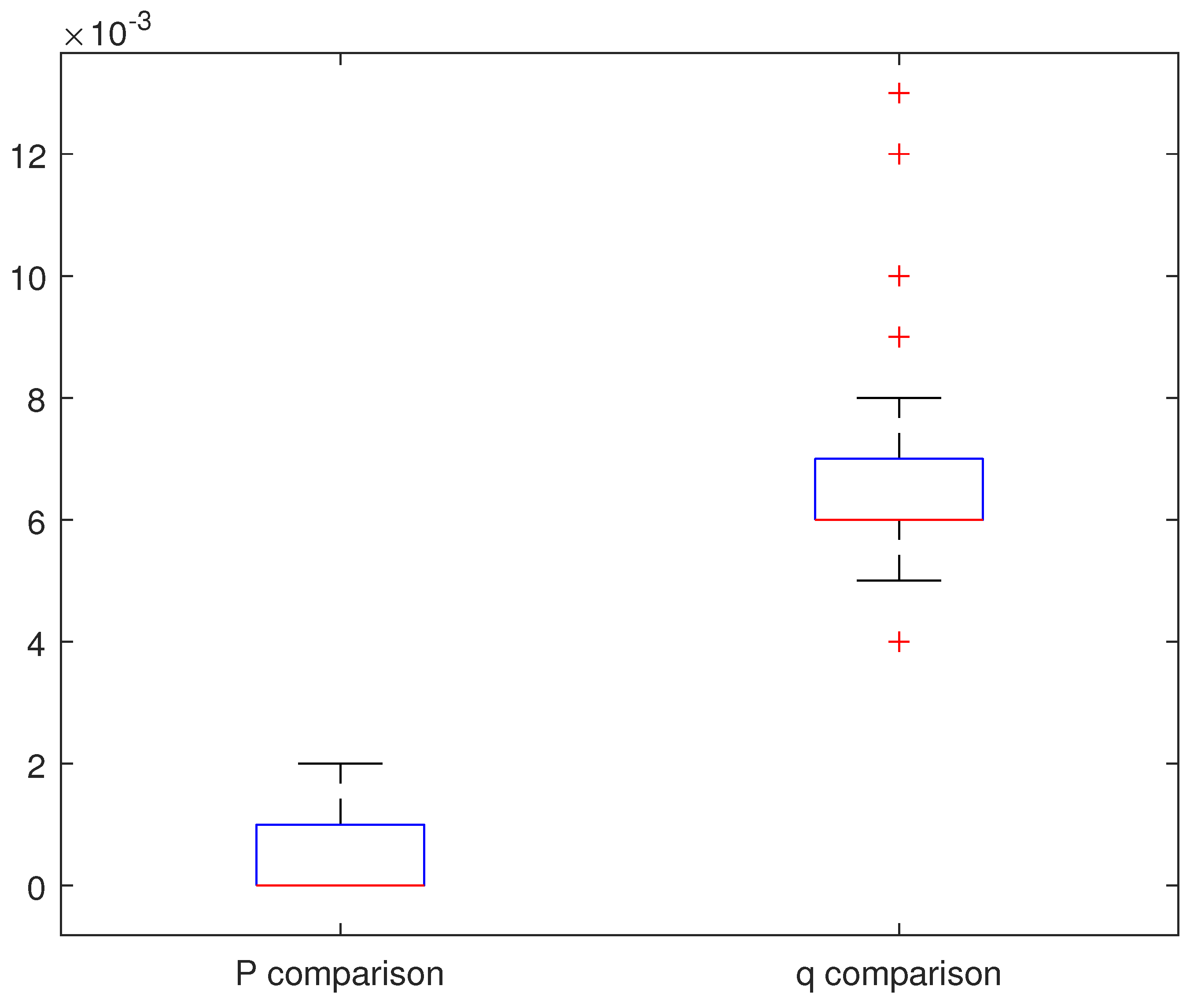
The two possibilities were compared. In terms of time, as seems natural, the first option took less than 1 ms while, the second took 6.4 ms as Figure 5 shows.
Although that difference is significant, option 2 presents two major advantages. First of all, it is valid even if the new configuration is far away from the robot’s present position (i.e., if a path is not followed but the robot is sent to different and distant positions). In addition, it makes it possible to measure the quality of the solutions given by the different nets and, in consequence, to estimate which of them are true solutions, but with another kinematic configuration, and which of them correspond to false tests.
Therefore, option 1 was chosen by default as the redundancy-avoidance method but, if the user specified when setting up the system that no path was followed, option 2 was executed.
3.3. The 3RRR Robot Used for Experiments
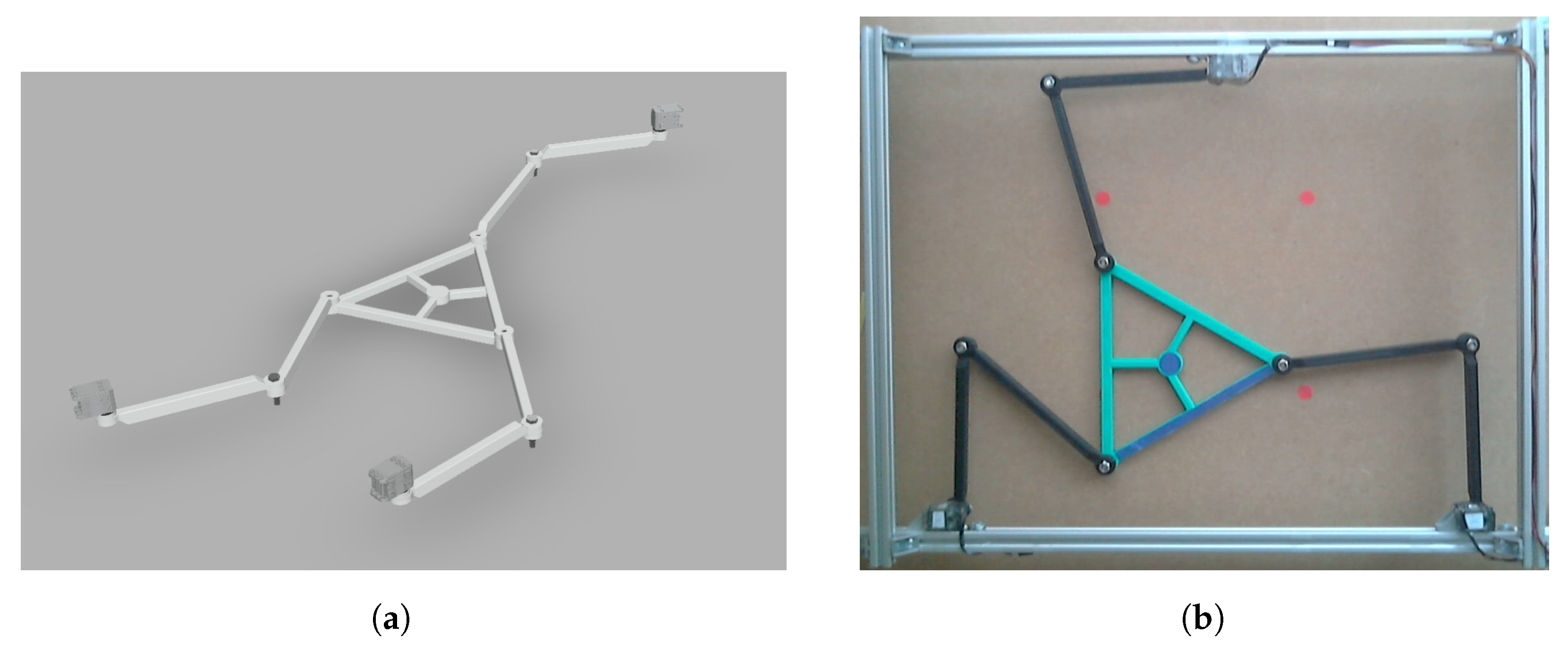
Although all the algorithms presented in this work are valid for any combination of the parameters shown in Table 1, in order to make the results analysis easier, they were implemented and validated on a real robot, whose physical characteristics are as follows:
Its bases, where the actuators are positioned, are located by making an equilateral triangle of the 50 cm sides; so its coordinates are:
A CAD model and a picture of the prototype, made by 3D-printing, can be seen in Figure 6.
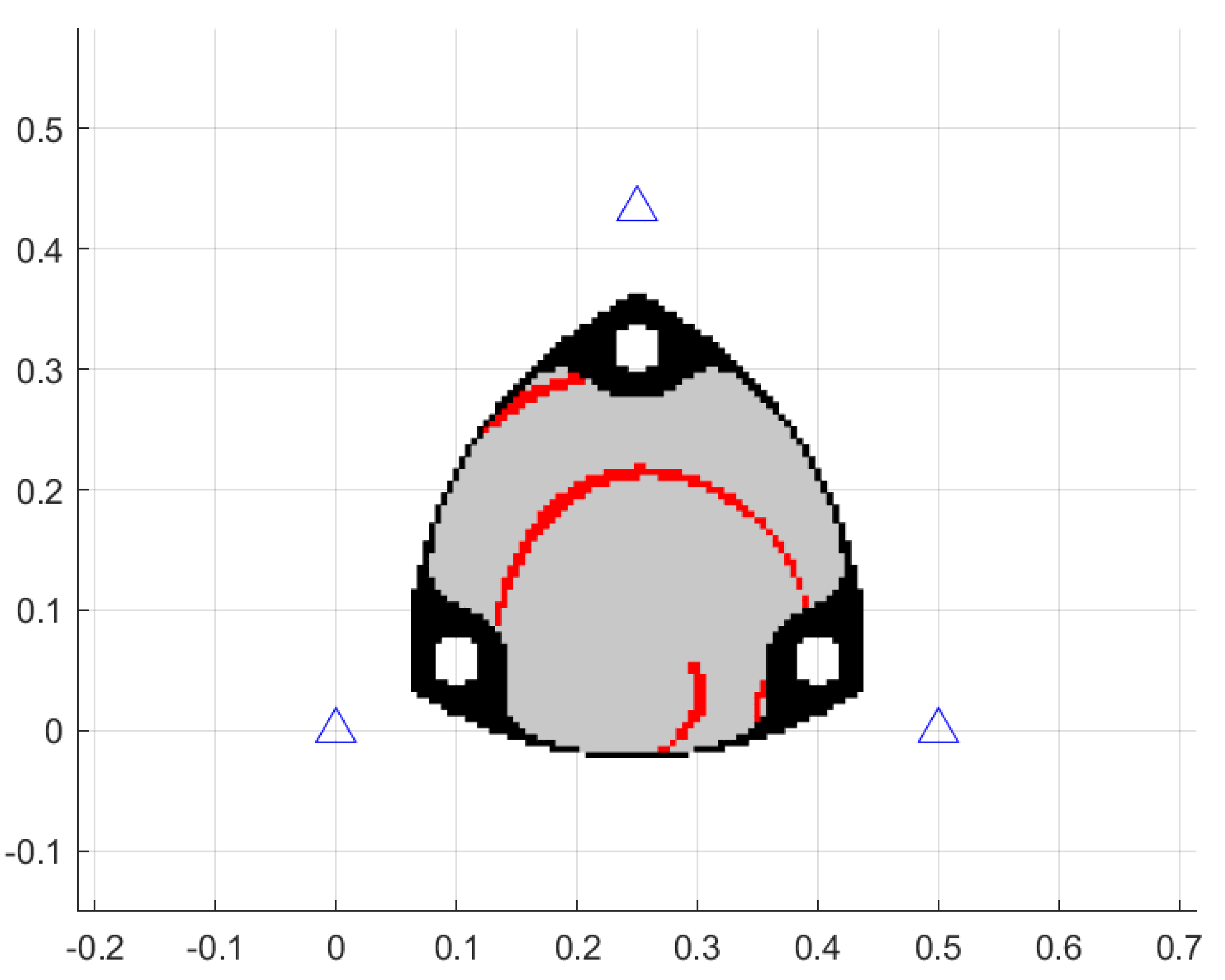
The robot workspace, when signs are taken in Equation (14), can be seen in Figure 7. Indirect singularities are drawn in black and direct singularities in red. The geometrical parameters of the manipulator, presented in Equations (22) and (23), were optimised to reach a workspace as free as possible from singular configurations.
All the algorithms were developed in Matlab R2019b. As mentioned when analysing the neural network training process, all the time measurements refer to the mentioned Intel Core i7 @2.6 GHz of 8 CPU processor.
4. Results
This section presents the most significant results achieved by each method. All of them are compared and the advantages and limitations are assessed.
Three experiments were carried out to compare the different methodologies introduced. First of all, the accuracy over the entire workspace was measured. Secondly, the time needed to complete the execution of the algorithm was compared. Finally, the three methods were used to follow different trajectories, such as a straight line and a circle, in order to contrast their performance over paths.
4.1. Accuracy
To carry out this experiment, 1036 points were used, which were uniformly distributed throughout the robot’s workspace, giving a resolution of approximately 96 points/. The robot was placed at each of these points and, using the IK model, the associated values were calculated. These values were then used as input to each model and a value of was obtained. The accuracy of each of the three methodologies was then measured as the distance between this value and the value at which the robot was actually placed, i.e., using the formula:
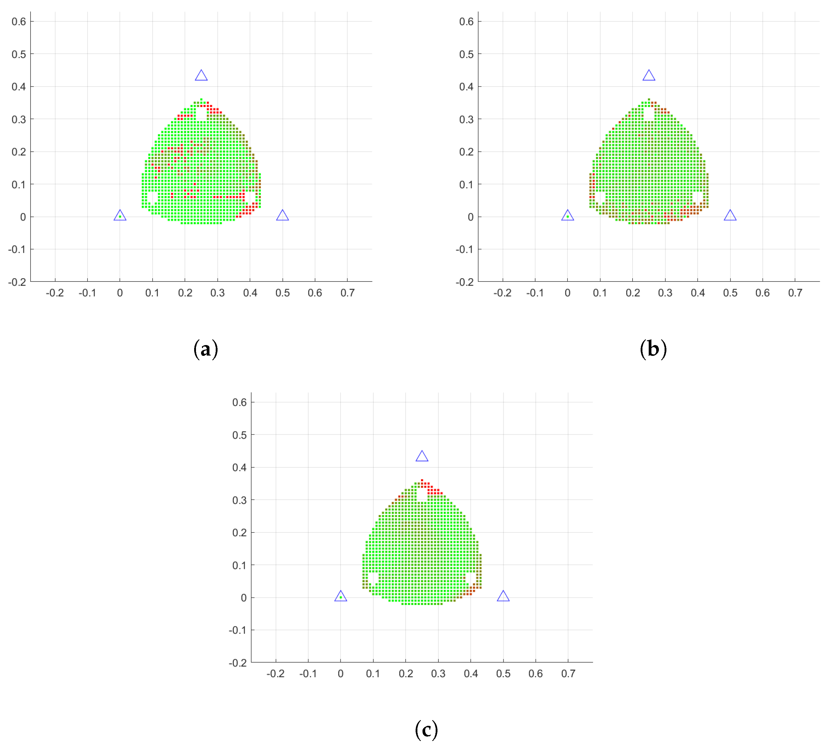
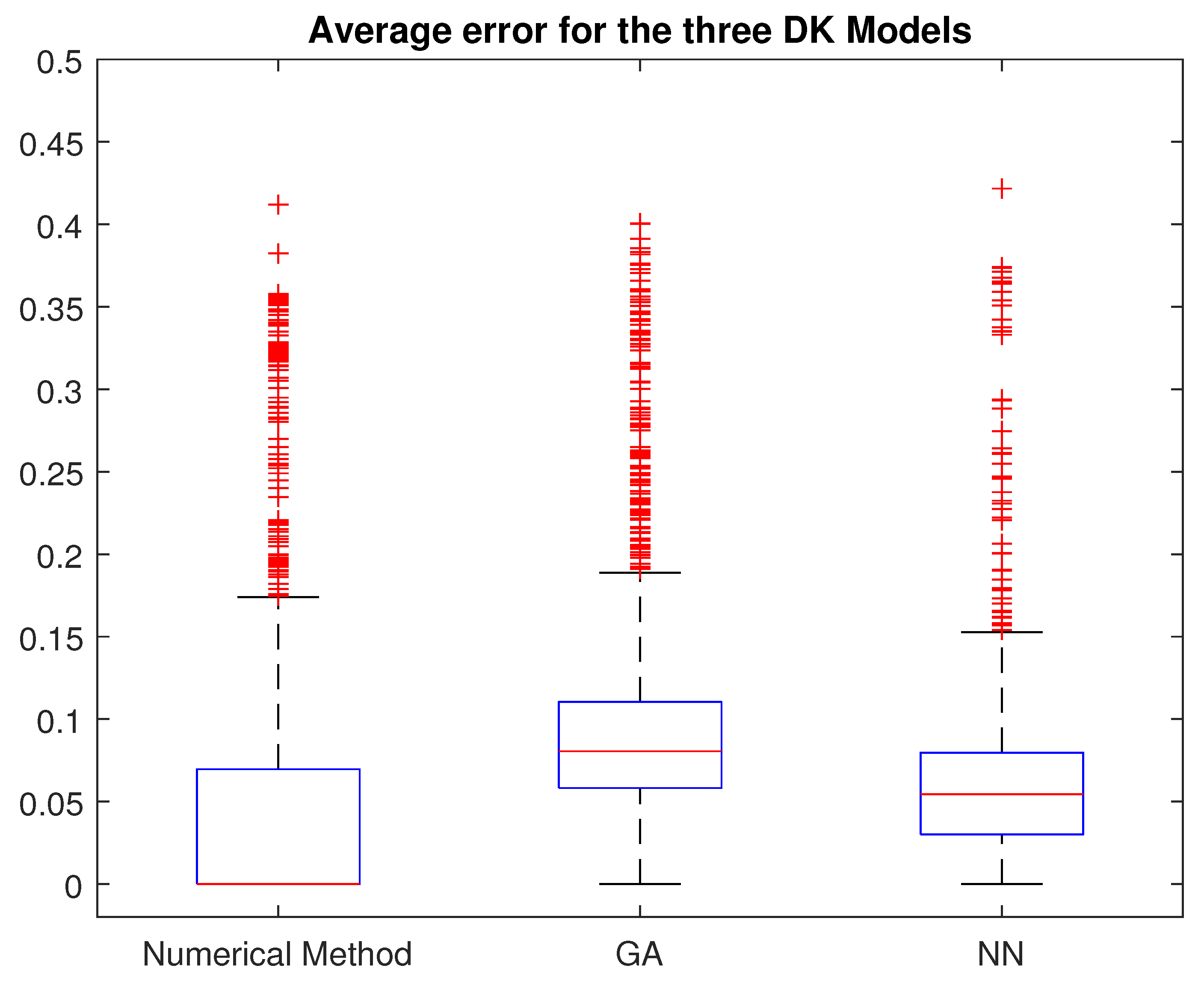
Figure 8 presents the accuracy over the workspace for the tree models. In Figure 9, the performance of the three methods, in terms of accuracy, is compared using a box plot. Table 4 summarises the most important statistical parameters of the experiment.
The numerical method was, looking at the results, the most precise model, although its repeatability, measured using the standard deviation or comparing the interquartile range of the results in Figure 9, was lower than the one provided by the neural network. This may have been caused by the high dependence on the point selected to start the iterations. As shown in Figure 8a, at some random points in the workspace, the algorithm was not able to converge, even in its neighbourhood.
The genetic algorithm offers, on average, lower accuracy than the other two. However, is important to note that, as Figure 9 shows, its typical values had maximum errors similar to the rest of the modelling techniques. The dispersion of the results was similar—even slightly below—the one reached in the numerical method, despite the inherent randomness of genetic algorithms. The points at the limits of the workspace show a poor accuracy. This may have been due to the difficulty to generate valid individuals in those regions. Crossover between two valid and good solutions or small mutations can easily give an individual outside the workspace.
Finally, the neural network model achieved a lower average accuracy than the numerical method but with higher repeatability, improving the results of the latter for the third quartile. Unlike the two previous models, Figure 8c, shows a uniform accuracy along all the points of the same region, with no significant bad results at random positions. In the vertex of the workspace, as happened with the genetic algorithm, the precision was lower than thar attained by the numerical model, probably due to the absence of training data. Some lack of accuracy was also appreciated in the centre of the workspace.
As explained in Section 2.2, in direct singularities, small movements in lead to large displacements in , which makes it interesting, when comparing FK algorithms, to evaluate the performance of all of them in regions close to the singular points. In this regard, it can be seen how several of the points marked in red in the centre of the workspace in Figure 8a correspond to the direct singularities displayed in Figure 7, which could be an indicator of a lack of robustness of the algorithm in these areas.
In order to carry out the comparison, 253 singular points of the workspace were selected and evaluated in the same way as for the entire workspace. The results are shown in Table 5.
As it can be seen, the numerical method suffered a considerable increase in its level of error. This was due to the Jacobian matrix of Equation (18), as a consequence of the large fluctuations of the derivatives at these points varying markedly, leading to instability problems. Therefore, it is necessary to note that, in 34.78% of the evaluated singular points, the algorithm did not converge, whereas this only occurred in less than 10% of the workspace when fully evaluated.
However, the two AI-based methodologies presented in this work, did not suffer, to the same extent, from these modelling shortcomings near the singularities. The genetic algorithm, as expected, was not affected in any way by direct singularities because no relation between the variations of and was considered in it. Its average accuracy in the 253 evaluated points was even better than in the entire workspace due to the fact that they were far from the border and, therefore, did not suffer from the problem of generating a significant number of invalid solutions.
The neural network presented similar—slightly, but not significantly lower—results to those when evaluating the entire workspace. As commented when presenting Figure 8c, some lack of precision was appreciated in the centre of the workspace, probably due to the fact that the net was not able to totally generalise the behaviour of the FK model in those specific areas, but the results are clearly better than the ones provided by the numerical method.
4.2. Time
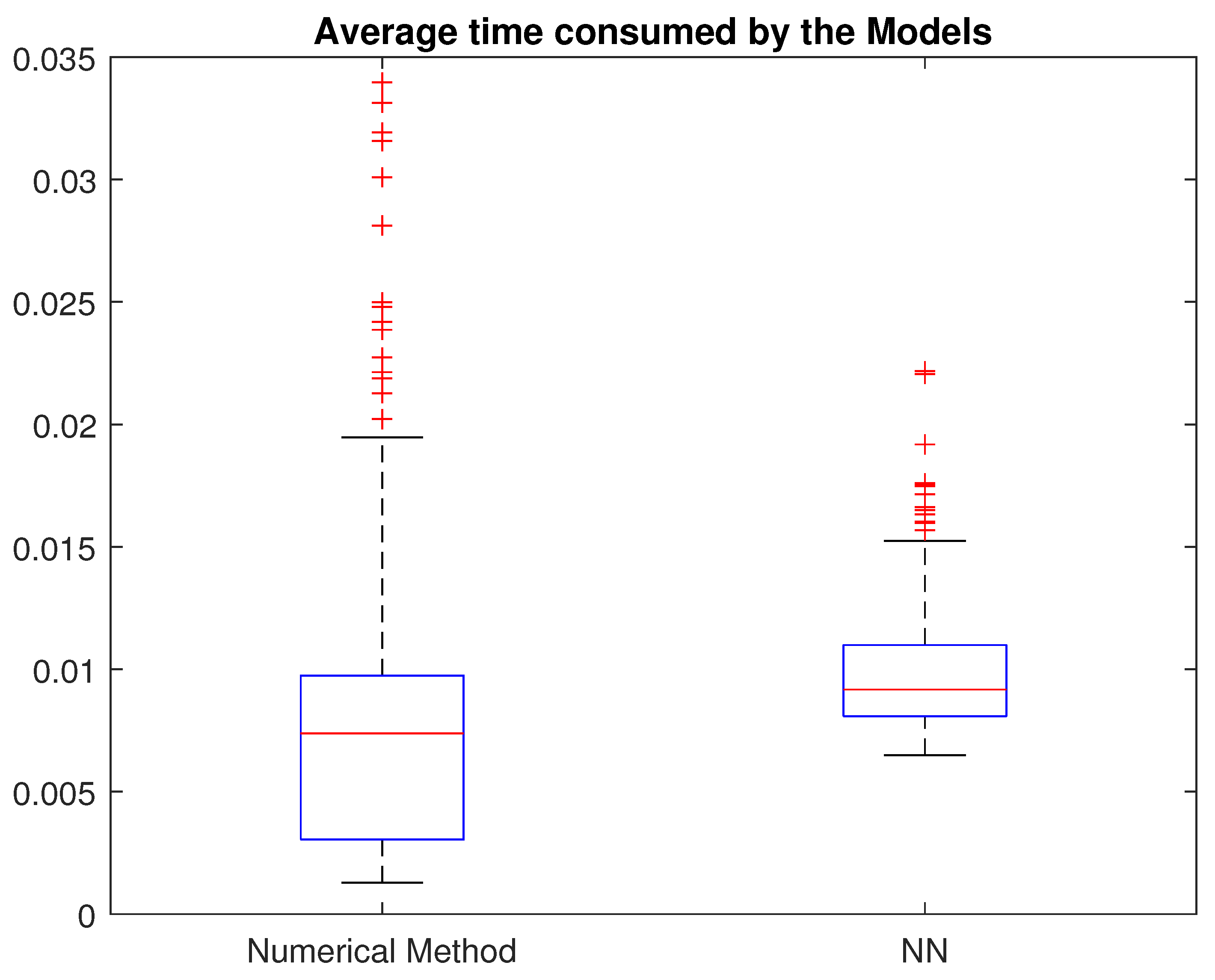
Time was measured over the whole workspace taking into account 100 different random points. Table 6 shows the performance of the three modelling methodologies. As can be observed, the execution of the genetic algorithm was in the order of seconds, while the other two took less than 15 ms. Both of them are compared in Figure 10. Although some significant difference can be observed, it can be ignored when working with real robots wherein even 200 ms is considered sufficiently fast.
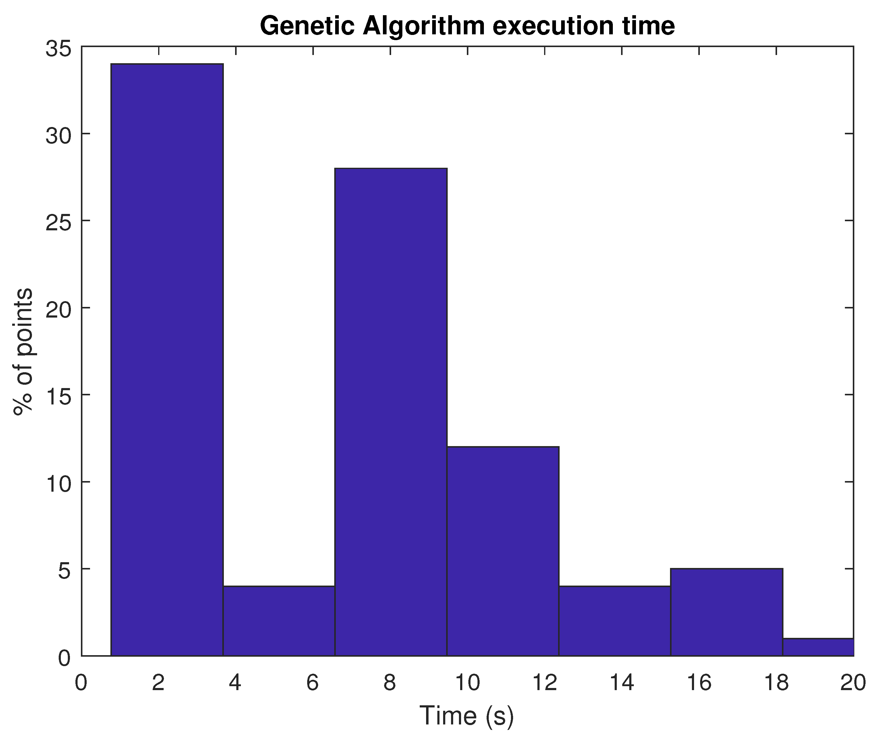
Concerning the genetic algorithm, regarding a limit of a speed that can be considered acceptable, it is important to note that this long execution time was primarily due to executions without early convergence. As Figure 11 shows, in more than a third of the situations, the model took less than 2 s to give the expected value of . Although this cannot be considered, contrary to what happened in the other two methodologies, as real-time values, these can be regarded as reasonable and feasible in applications where time is not a critical parameter.
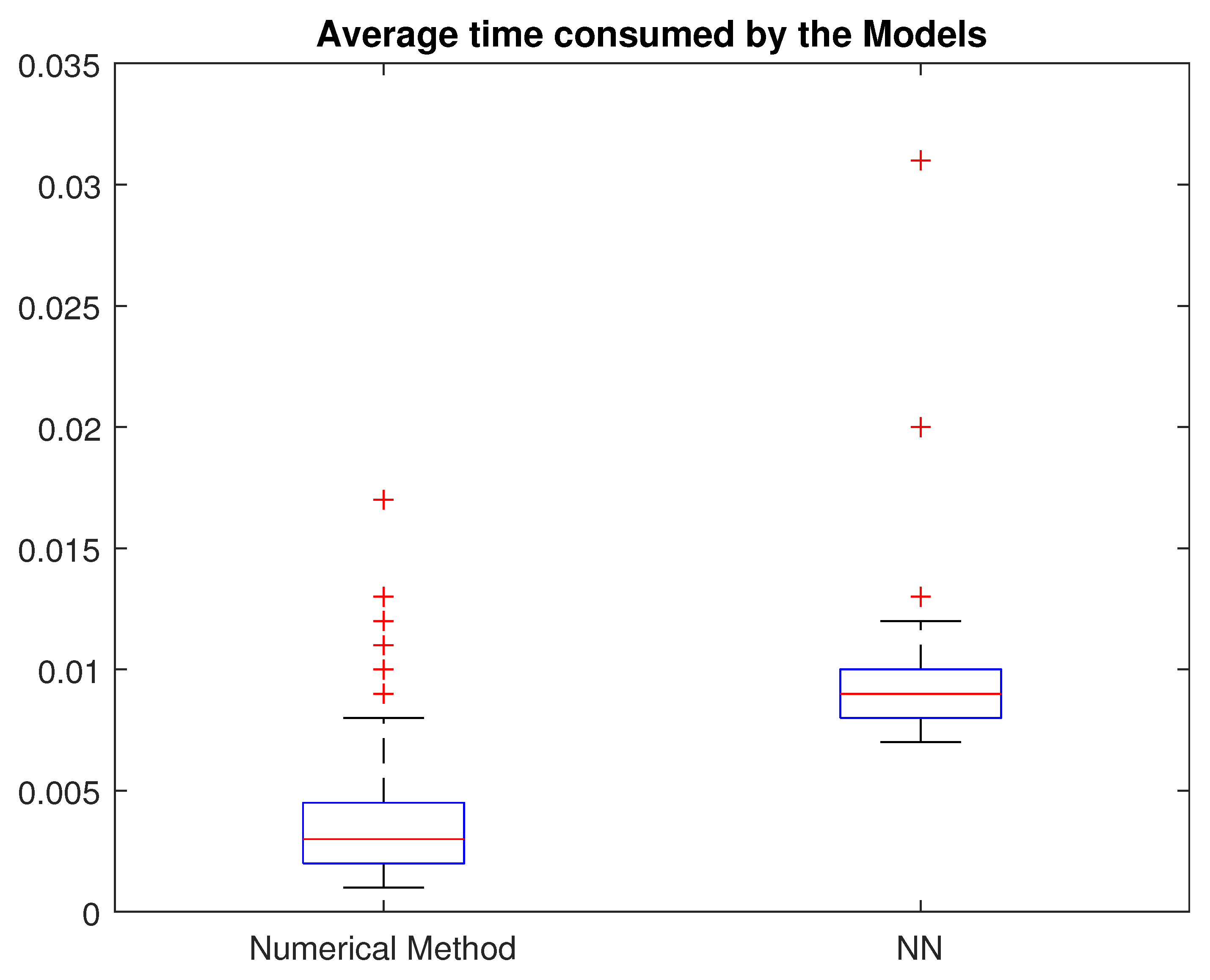
Time was also measured in the same set of singular points as that used in the case of accuracy. As Figure 12 shows, the average consumed time was very similar in the numerical method and using the neural network. Although the first was sometimes able to present faster results, it is also true that its worst-case scenarios were slower than those of the net. The highest number of iterations required for the numerical method is, in consequence, reflected in terms of time, whereas the neural network always took the same amount of time to predict the result.
4.3. Path Following
Finally, a test was designed to make the robot follow previously defined trajectories. No type of kinematic control was carried out, but rather the robot was given a series of points to achieve, in joint coordinates, and then the positions reached were studied and compared with those which, theoretically, should have been reached.
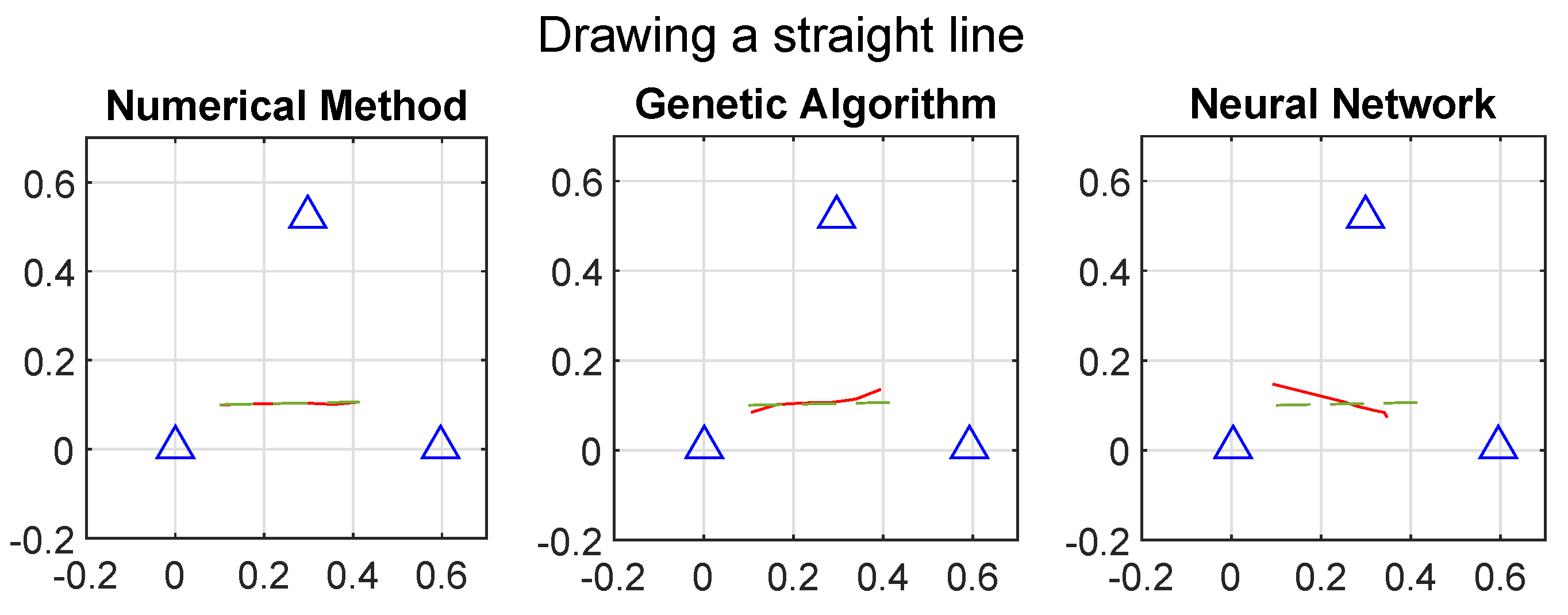
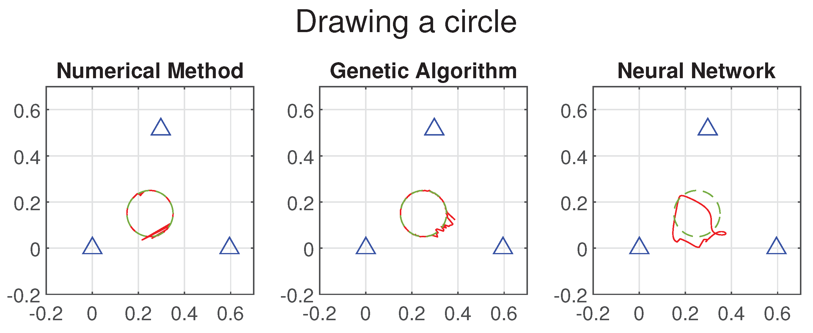
Two paths were studied: a circle and a straight line. They were defined in the task space and converted to coordinates using the IK model. The results of the three methodologies trying to follow these paths can be found in Figure 13 and Figure 14.
For both the numerical and genetic algorithm methods, the initial point for each step of the path was the present point of the robot multiplied by a number randomly taken from a normal distribution . Non-convergent values were removed from the results. This was an attempt to emulate a situation of path planning where the values of were captured by the sensors with some noise.
Because these two methods take, as initial point, the current position of the robot, they outperformed the results obtained during the experiments that took place in the whole workspace. As Table 7 shows, both the mean and standard deviation for the numerical method and the genetic algorithm were considerably lower when following paths, while the error values for the neural network can be considered similar.
5. Discussion
The different experiments carried out showed, first of all, that both methodologies can achieve results similar to the numerical method introduced in [26], but without the need for additional mathematical developments which, moreover, are not intuitive and cannot be systematically transferred to other types of parallel robot. Furthermore, the algorithms developed in this work do not, in contrast to the numerical method, show worse results in singular regions.
However, it can also be said that the two methodologies have significant differences, in terms of accuracy and time, and their areas of application do not fully coincide. This section will discuss the advantages and disadvantages of both methodologies and will analyse when the use of one or the other is preferable.
5.1. Genetic Algorithm
The experiments revealed that the genetic algorithm proposed in this study is both slower compared to the other two methods and is unable to achieve the same level of precision on average. This limitation arises because the genetic algorithm needs to calculate the IK model a total of NRobots times at each generation. While it is conceptually straightforward and highly adaptable to other configurations, it is simultaneously time-intensive. Reducing the number of robots or generations results in a reduced accuracy, rendering the outcomes unacceptable in most cases. With the fine-tuned parameters in this study, the results remained within acceptable ranges: when early convergence was not achieved, movements were attained approximately every 3 s.
However, as mentioned earlier, the genetic algorithm demonstrates a significant improvement in its results when it comes to path following. This improvement is attributed to the fact that individuals are generated around the robot’s current position. Consequently, the probability of generating a favourable individual before the NIter iterations are exhausted, where tolerances are smaller, and accuracy is higher, increases. As a result, not only are benefits in terms of accuracy achieved, but also in terms of time. It was demonstrated that even with slight deviations in defining the current position, effective path tracking can be accomplished.
The challenge of working with points near the boundaries of the workspace within a reasonable time frame was effectively addressed by introducing random generation when a large number of invalid individuals are generated. In the centre of the workspace, where direct singularities occur, the genetic algorithm stands out as the only methodology that is entirely independent of them, with no decrease in accuracy being evident.
5.2. Neural Network
The neural network model, on the other hand, achieves similar practical performance to the numerical method. Once trained, it provides an FK solution in approximately 11 ms. Although this is more than twice the average time consumed by the numerical method, Figure 10 illustrates that this difference cannot be considered significant. Moreover, these time intervals are not critical when considering actuator movements. Furthermore, in singular regions, as depicted in Figure 12, the average performance of both methods is similar, with the worst cases being faster for the neural network than for the numerical method.
In terms of accuracy, more consistent values were obtained here. Unlike the other two methods, which rely on a random component, the neural network can be considered, in a certain sense, as a continuum model, where no isolated points offer better or worse results than the ones in their vicinity. The precision achieved in a region remains uniform within that region. Comparing the numerical method and the neural network in Figure 8 shows that the latter has neither brilliant green points (points with a very good precision) nor brilliant red points (points with a very low accuracy), but everything is much more modulated. This phenomenon arises because the numerical method, due to its iterative reliance on a Jacobian matrix, encounters notable difficulties in converging near singularities.
As expected, the corners of the workspace, where fewer points are available for training, offered worse results than the average. However, this effect was relatively minor compared to the genetic algorithm and was similar to the numerical method, which also exhibits instabilities in this region. There was a small reduction in accuracy in the centre of the workspace, probably due to singularities, which can make net interpolation difficult.
Furthermore, the accuracy of the model is not related to the size of the robot’s workspace, unlike what happens in both the numerical method, where points that are too far away may not be reached after 100 iterations, and the genetic algorithm, where a bigger workspace will generate more dispersed individuals, which reduces the likelihood of quickly finding a very accurate solution. For this model, larger workspaces imply longer training times if the same dataset resolution (and consequently accuracy) is maintained, but once trained, the solution is provided in a matter of milliseconds.
Regarding path tracking, the proximity between the points does not offer an advantage here, because each call to the method is independent from the previous ones and cannot be conditioned by the robot’s current position. Although errors are generally acceptable, the shapes of the figures are more difficult to appreciate. Nevertheless, if no online planning is required, some path correction methodologies can be implemented.
Moreover, compared to the other two methodologies, neural networks offer two major advantages, although they have not fully been developed in this work. On the one hand, the model, as implemented here, can be easily prepared to handle multiple solutions. Using the second of the criteria presented in Section 3.2.3 and experimentally fixing a maximum error threshold between the values of the desired and the obtained using the IK model, various solutions can be returned.
On the other, this methodology can be implemented without the necessity of any form of kinematic modelling. Because training of the net is based on data, which relate the values of with the corresponding ; if it is possible to capture them using a vision system and reading the actuators’ positions, a dataset can be generated. It is true that a large amount of data are required, but the idea can be very useful when obtaining the robot kinematics is challenging.
6. Conclusions
Although solving the FK modelling of parallel manipulators is a challenge with no analytical solution, AI-based methodologies have demonstrated their ability to achieve good results in tackling this task. The two approaches introduced in this work—a genetic algorithm and a neural network—have shown that they can produce results comparable in terms of accuracy and time to existing techniques in the literature.
Furthermore, these AI-based approaches address the two main challenges associated with the numerical method. Firstly, they do not require the development of non-intuitive mathematical reasoning. By solely using the IK model, which can be easily obtained through geometric reasoning, both methodologies correctly predict the robot’s position based on the actuator angles. Secondly, their performance is not compromised when operating near singular points, which is a significant advantage as these points are abundant in parallel planar robots and are typically located in the centre of the workspace. However, the differences in methodology make each model preferable for different situations.
The genetic algorithm is useful for applications where trajectory tracking is a priority (because the robot’s current position is taken as reference) and where time is not a limiting factor (due to the computational cost of the method and its associated randomness, which can lead to high convergence times in some situations). It is also advisable to use this technique in regions that are not too close to the border of the workspace. Several of the applications discussed in the Introduction, such as high-precision tasks or those linked to rehabilitation exercises—especially in its early stages—fit within these characteristics. It must also be said, given the markedly research-oriented nature of 3RRR robots, that the genetic algorithm presented here is valid whatever the values of the 15 geometric parameters of the robot (the lengths of the six bars, the length of platform sides, and the position of the actuators), without the need for additional training or modifications.
The neural network model, for its part, is a reliable solution in most cases. It is neither conditioned by the current robot position nor influenced, once the training is completed, by random aspects. As a result, it achieves consistent accuracies over the entire workspace, without isolated points or specific regions where it performs significantly worse—except at the boundary, where a larger number of training points can compensate for this limitation. If no path following is desired (or offline corrections are feasible) and a guaranteed maximum error threshold is needed, this modelling technique is a valuable option to consider.
Moreover, it can be very useful when high accuracies are desired in robots with large working spaces. The only requirement is to have a bigger dataset for the training process. Furthermore, compared to other existing techniques, it allows the multiplicity of solutions to be considered and can be trained experimentally, without even needing to use the IK model.
The success of the two techniques demonstrated in this work opens the door to implementing it in more parallel manipulator typologies. A future line of interest could be the comparison of both methodologies in terms of their ease of application to other planar parallel robotic structures.
Author Contributions
Conceptualization, A.B. and J.F.G.-S.; methodology, J.F.G.-S.; software, J.F.G.-S.; validation, J.F.G.-S.; formal analysis, A.B. and J.F.G.-S.; investigation, J.F.G.-S. and A.B.; resources, A.B.; data curation, J.F.G.-S.; writing—original draft preparation, J.F.G.-S.; writing—review and editing, A.B. and J.F.G.-S.; visualization, J.F.G.-S. and A.B.; supervision, A.B.; project administration, A.B.; funding acquisition, A.B. All authors have read and agreed to the published version of the manuscript.
Funding
This research was possible thanks to the financing of “Ayudas para contratos predoctorales para la realización del doctorado con mención internacional en sus escuelas, facultad, centros e institutos de I+D+i”, funded by Programa Propio I+D+i 2022 from Universidad Politécnica de Madrid and RoboCity2030-DIH-CM, Madrid Robotics Digital Innovation Hub, S2018/NMT-4331, funded by “Programas de Actividades I+D en la Comunidad Madrid”.
Data Availability Statement
The data and the code presented in this study are openly available at https://github.com/Robcib-GIT/3RRR (accessed on 11 October 2023).
Conflicts of Interest
The authors declare no conflict of interest. The funders had no role in the design of the study; in the collection, analyses, or interpretation of data; in the writing of the manuscript; or in the decision to publish the results.
Abbreviations
The following abbreviations are used in this manuscript:
| FK | Forward Kinematics |
| IK | Inverse Kinematics |
| GA | Genetic Algorithm |
| NN | Neural Network |
| AI | Artificial Intelligence |
| MSE | Mean Squared Error |
References
- Jin, Y.; Chanal, H.; Paccot, F. Parallel Robots; Springer: London, UK, 2015; pp. 2091–3487. [Google Scholar] [CrossRef]
- Hamdoun, O.; El Bakkali, L.; Baghli, F.Z. Optimal Trajectory Planning of 3RRR Parallel Robot Using Ant Colony Algorithm. In Robotics and Mechatronics; Zeghloul, S., Laribi, M.A., Gazeau, J.P., Eds.; Springer: Cham, Switzerland, 2016; pp. 131–139. [Google Scholar]
- Huynh, B.P.; Kuo, Y.L. Dynamic filtered path tracking control for a 3RRR robot using optimal recursive path planning and vision-based pose estimation. IEEE Access 2020, 8, 174736–174750. [Google Scholar] [CrossRef]
- Merlet, J.P. Direct kinematics of planar parallel manipulators. In Proceedings of the IEEE International Conference on Robotics and Automation, Minneapolis, MN, USA, 22–28 April 1996; Volume 4, pp. 3744–3749. [Google Scholar] [CrossRef]
- Gallardo-Alvarado, J.; Tinajero-Campos, J.H.; Sánchez-Rodríguez, A. Kinematics of a configurable manipulator using screw theory. Rev. Iberoam. AutomáTica InformáTica Ind. 2021, 18, 58–67. [Google Scholar] [CrossRef]
- Mora, J.P.; Samper, J.; Rodriguez, C.F. Bayesian optimization study for energy consumption reduction of a parallel robot during pick and place tasks. Rev. Iberoam. AutomáTica InformáTica Ind. 2023, 20, 1–12. [Google Scholar] [CrossRef]
- Stewart, D. A Platform with Six Degrees of Freedom. Proc. Inst. Mech. Eng. 1965, 180, 371–386. [Google Scholar] [CrossRef]
- Yin, Z.; Qin, R.; Liu, Y. A New Solving Method Based on Simulated Annealing Particle Swarm Optimization for the Forward Kinematic Problem of the Stewart–Gough Platform. Appl. Sci. 2022, 12, 7657. [Google Scholar] [CrossRef]
- Guagliumi, L.; Berti, A.; Monti, E.; Carricato, M. Design Optimization of a 6-DOF Cable-Driven Parallel Robot for Complex Pick-and-Place Tasks. In ROMANSY 24—Robot Design, Dynamics and Control; Kecskeméthy, A., Parenti-Castelli, V., Eds.; Springer: Cham, Switzerland, 2022; pp. 283–291. [Google Scholar]
- Qin, X.; Shi, M.; Hou, Z.; Li, S.; Li, H.; Liu, H. Analysis of 3-DOF Cutting Stability of Titanium Alloy Helical Milling Based on PKM and Machining Quality Optimization. Machines 2022, 10, 404. [Google Scholar] [CrossRef]
- Gagliardini, L.; Caro, S.; Gouttefarde, M.; Wenger, P.; Girin, A. A reconfigurable cable-driven parallel robot for sandblasting and painting of large structures. In Cable-Driven Parallel Robots: Proceedings of the Second International Conference on Cable-Driven Parallel Robots; Springer: Berlin/Heidelberg, Germany, 2015; pp. 275–291. [Google Scholar]
- Mohajer, N.; Abdi, H.; Nelson, K.; Nahavandi, S. Vehicle motion simulators, a key step towards road vehicle dynamics improvement. Veh. Syst. Dyn. 2015, 53, 1204–1226. [Google Scholar] [CrossRef]
- Gosselin, C.M.; Sefrioui, J. Polynomial solutions for the direct kinematic problem of planar three-degree-of-freedom parallel manipulators. In Proceedings of the Fifth International Conference on Advanced Robotics’ Robots in Unstructured Environments, Pisa, Italy, 19–22 June 1991. [Google Scholar]
- Gosselin, C.M.; Merlet, J.P. The direct kinematics of planar parallel manipulators: Special architectures and number of solutions. Mech. Mach. Theory 1994, 29, 1083–1097. [Google Scholar] [CrossRef]
- Arakelian, V.; Smith, M. Design of planar 3-DOF 3-RRR reactionless parallel manipulators. Mechatronics 2008, 18, 601–606. [Google Scholar] [CrossRef]
- Zubizarreta, A.; Cabanes, I.; Marcos, M.; Pinto, C.; Portillo, E. Redundant dynamic modelling of the 3RRR parallel robot for control error reduction. In Proceedings of the 2009 European Control Conference (ECC), Budapest, Hungary, 23–26 August 2009; pp. 2205–2210. [Google Scholar] [CrossRef]
- Popov, D.; Klimchik, A. Optimal Planar 3RRR Robot Assembly Mode and Actuation Scheme for Machining Applications. IFAC-PapersOnLine 2018, 51, 734–739. [Google Scholar] [CrossRef]
- Wu, J.; Wang, J.; Wang, L.; You, Z. Performance comparison of three planar 3-DOF parallel manipulators with 4-RRR, 3-RRR and 2-RRR structures. Mechatronics 2010, 20, 510–517. [Google Scholar] [CrossRef]
- Kucuk, S. A dexterity comparison for 3-DOF planar parallel manipulators with two kinematic chains using genetic algorithms. Mechatronics 2009, 19, 868–877. [Google Scholar] [CrossRef]
- Cardona, M.N. Similarity law for the design and workspace optimization of 3RRR planar parallel robots. In Proceedings of the 2014 IEEE Central America and Panama Convention, CONCAPAN 2014, Panama, Panama, 12–14 November 2014; pp. 1–6. [Google Scholar] [CrossRef]
- Infante-Jacobo, M.; Valdez, S.I.; Hernández, E.; Chavez-Conde, E.; Botello-Aceves, S. Optimización de la Estructura-Control de un Robot Paralelo Planar 3RRR usando Algoritmos Evolutivos, Matlab-Simulink y SimWise 4D. Comun. Del CIMAT 2017. Available online: https://famat.cimat.mx/BiblioAdmin/RTAdmin/reportes/enlinea/I-17-02.pdf (accessed on 11 October 2023).
- Yime, E.; Saltarén, R.J.; Roldán Mckinley, J.A. Inverse Dynamics of Parallel Robots: A tutorial with Lie algebra. Rev. Iberoam. Autom. Inform. Ind. 2023, 20, 327–346. [Google Scholar] [CrossRef]
- Cardona, M. Dimensional Synthesis of 3RRR Planar Parallel Robots for Well-Conditioned Workspace. IEEE Lat. Am. Trans. 2015, 13, 409–415. [Google Scholar] [CrossRef]
- Rodelo, M.; Polo, S.; Duque, J.; Villa, J.L.; Yime, E. Robust adaptive control of a planar 3RRR parallel robot for trajectory-tracking applied to crouch gait cycle in children with cerebral palsy. In Proceedings of the 2019 IEEE 4th Colombian Conference on Automatic Control (CCAC), Medellin, Colombia, 15–18 October 2019. [Google Scholar] [CrossRef]
- Oetomo, D.; Liaw, H.C.; Alici, G.; Shirinzadeh, B. Direct kinematics and analytical solution to 3RRR parallel planar mechanisms. In Proceedings of the 9th International Conference on Control, Automation, Robotics and Vision, 2006, ICARCV ’06, Singapore, 11–13 December 2006. [Google Scholar] [CrossRef]
- Abo-Shanab, R.F. An Efficient Method for Solving the Direct Kinematics of Parallel Manipulators Following a Trajectory. J. Autom. Control. Eng. 2014, 2, 228–233. [Google Scholar] [CrossRef]
- Peidró, A.; Tendero, C.; Marín, J.M.; Gil, A.; Payá, L.; Reinoso, Ó. m-PaRoLa: A Mobile Virtual Laboratory for Studying the Kinematics of Five-bar and 3RRR Planar Parallel Robots. IFAC-PapersOnLine 2018, 51, 178–183. [Google Scholar] [CrossRef]
- Bohigas, O.; Henderson, M.E.; Porta, J.M. Planning Singularity-Free Paths on Closed-Chain Manipulators. IEEE Trans. Robot. 2013, 29, 888–898. [Google Scholar] [CrossRef]
- Peidró, A.; Payá, L.; Cebollada, S.; Román, V.; Reinoso, Ó. Solution of the Forward Kinematics of Parallel Robots Based on Constraint Curves. In Informatics in Control, Automation and Robotics; Gusikhin, O., Madani, K., Zaytoon, J., Eds.; Springer: Cham, Switzerland, 2022; pp. 386–409. [Google Scholar]
- Rodelo, M.; Villa, J.L.; Duque, J.; Yime, E. Kinematic Analysis and Performance of a Planar 3RRR Parallel Robot with Kinematic Redundancy using Screw Theory. In Proceedings of the 2018 IEEE 2nd Colombian Conference on Robotics and Automation (CCRA), Barranquilla, Colombia, 1–3 November 2018; pp. 1–6. [Google Scholar] [CrossRef]
- Omran, A.; Bayoumi, M.; Kassem, A.; El-Bayoumi, G. Optimal Forward Kinematics Modeling of a Stewart Manipulator using Genetic Algorithms. Jordan J. Mech. Ind. Eng. 2009, 3, 280–293. [Google Scholar]
- Momani, S.; Abo-Hammour, Z.S.; Alsmadi, O.M. Solution of inverse kinematics problem using genetic algorithms. Appl. Math. Inf. Sci. 2016, 10, 225–233. [Google Scholar] [CrossRef]
- Wu, D.; Zhang, W.; Qin, M.; Xie, B. Interval Search Genetic Algorithm Based on Trajectory to Solve Inverse Kinematics of Redundant Manipulators and Its Application. In Proceedings of the 2020 IEEE International Conference on Robotics and Automation (ICRA), Paris, France, 31 May–31 August 2020; pp. 7088–7094. [Google Scholar] [CrossRef]
- Lee, C.T.; Chang, J.Y.J. A Workspace-Analysis-Based Genetic Algorithm for Solving Inverse Kinematics of a Multi-Fingered Anthropomorphic Hand. Appl. Sci. 2021, 11, 2668. [Google Scholar] [CrossRef]
- Li, S.; Zhang, Y.; Jin, L. Kinematic Control of Redundant Manipulators Using Neural Networks. IEEE Trans. Neural Netw. Learn. Syst. 2017, 28, 2243–2254. [Google Scholar] [CrossRef] [PubMed]
- Tavassolian, F.; Khotanlou, H.; Varshovi-Jaghargh, P. Forward Kinematics Analysis of a 3-PRR Planer Parallel Robot Using a Combined Method Based on the Neural Network. In Proceedings of the 2018 8th International Conference on Computer and Knowledge Engineering (ICCKE), Mashhad, Iran, 25–26 October 2018; pp. 320–325. [Google Scholar] [CrossRef]
- Zubizarreta, A.; Larrea, M.; Irigoyen, E.; Cabanes, I.; Portillo, E. Real time direct kinematic problem computation of the 3PRS robot using neural networks. Neurocomputing 2018, 271, 104–114. [Google Scholar] [CrossRef]
- Prado, A.; Zhang, H.; Agrawal, S.K. Artificial Neural Networks to Solve Forward Kinematics of a Wearable Parallel Robot with Semi-rigid Links. In Proceedings of the IEEE International Conference on Robotics and Automation, Xi’an, China, 30 May–5 June 2021; pp. 14524–14530. [Google Scholar] [CrossRef]
- Wagaa, N.; Kallel, H.; Mellouli, N. Analytical and deep learning approaches for solving the inverse kinematic problem of a high degrees of freedom robotic arm. Eng. Appl. Artif. Intell. 2023, 123, 106301. [Google Scholar] [CrossRef]
- Lopez-Franco, C.; Hernandez-Barragan, J.; Alanis, A.Y.; Arana-Daniel, N. A soft computing approach for inverse kinematics of robot manipulators. Eng. Appl. Artif. Intell. 2018, 74, 104–120. [Google Scholar] [CrossRef]
- Gosselin, C.; Angeles, J. Singularity analysis of closed-loop kinematic chains. IEEE Trans. Robot. Autom. 1990, 6, 281–290. [Google Scholar] [CrossRef]
- Marchi, T.; Mottola, G.; Porta, J.M.; Thomas, F.; Carricato, M. Position and Singularity Analysis of a Class of Planar Parallel Manipulators with a Reconfigurable End-Effector. Machines 2021, 9, 7. [Google Scholar] [CrossRef]
- Chen, X.; Xie, F.; Liu, X.J. Singularity analysis of the planar 3-RRR parallel manipulator considering the motion/force transmissibility. In Proceedings of the Intelligent Robotics and Applications: 5th International Conference, ICIRA 2012, Montreal, QC, Canada, 3–5 October 2012; Volume 7506, pp. 250–260. [Google Scholar] [CrossRef]
- Bohigas, O.; Manubens, M.; Lluis, R. Singularities of Robot Mechanisms. Numerical Computation and Avoidance Path Planning; Springer International Publishing: Berlin/Heidelberg, Germany, 2018. [Google Scholar]
- Hamdoun, O.; Baghli, F.Z.; Bakkali, L.E.L. Inverse kinematic Modeling of 3RRR Parallel Robot. In Proceedings of the CFM 2015—22ème Congrès Français de Mécanique, Lyon, France, 24–28 August 2015. [Google Scholar]
- Pulloquinga, J.L.; Escarabajal, R.J.; Valera, Á.; Vallés, M.; Mata, V. A Type II singularity avoidance algorithm for parallel manipulators using output twist screws. Mech. Mach. Theory 2023, 183, 105282. [Google Scholar] [CrossRef]
- Huang, M. Design of a Planar Parallel Robot for Optimal Workspace and Dexterity. Int. J. Adv. Robot. Syst. 2011, 8, 49. [Google Scholar] [CrossRef]
- Kardan, I.; Akbarzadeh, A. An improved hybrid method for forward kinematics analysis of parallel robots. Adv. Robot. 2015, 29, 401–411. [Google Scholar] [CrossRef]
- Nazari, A.A.; Hasani, A.; Beedel, M. Screw theory-based mobility analysis and projection-based kinematic modeling of a 3-CRRR parallel manipulator. J. Braz. Soc. Mech. Sci. Eng. 2018, 40, 357. [Google Scholar] [CrossRef]
- Zou, S.; Liu, H.; Liu, Y.; Yao, J.; Wu, H. Singularity Analysis and Representation of 6DOF Parallel Robot Using Natural Coordinates. J. Robot. 2021, 2021, 9935794. [Google Scholar] [CrossRef]
- Ji, P.; Wu, H. An efficient approach to the forward kinematics of a planar parallel manipulator with similar platforms. IEEE Trans. Robot. Autom. 2002, 18, 647–649. [Google Scholar] [CrossRef]
- Gallardo-Alvarado, J. Unified infinitesimal kinematics of a 3-RRR/PRR six-degree-of-freedom parallel-serial manipulator. Meccanica 2023, 58, 795–811. [Google Scholar] [CrossRef]
Figure 1.
3RRR parallel manipulator.

Figure 2.
Definition of the central platform parameters.

Figure 3.
Eight possible solutions of the inverse kinematic model. Source: authors.

Figure 4.
Results of the network training. (a) Regression plot for the last iteration. (b) Error histogram for the last iteration.
Figure 4.
Results of the network training. (a) Regression plot for the last iteration. (b) Error histogram for the last iteration.

Figure 5.
Comparison of methods to manage redundancy in NN modelling. The boxes cover all samples in the second and third quartile, while the red lines indicate the median of the distribution. Whisker length corresponds to 1.5 the interquartile range (IQR) or to the minimum and maximum value of the series if they are reached before. Outliers are marked as red crosses.

Figure 6.
3RRR robot used for experiments. (a) CAD model. (b) Real robot.

Figure 7.
Workspace of the robot used for the experiments. Inverse singularities are drawn in black and direct singularities in red. The blue triangles indicate the position of each of the three bases .
Figure 7.
Workspace of the robot used for the experiments. Inverse singularities are drawn in black and direct singularities in red. The blue triangles indicate the position of each of the three bases .

Figure 8.
Accuracy across the entire workspace for each model. Greener dots indicate higher accuracy and redder dots indicate higher error. (a) Numerical method. (b) Genetic algorithm. (c) Neural network.
Figure 8.
Accuracy across the entire workspace for each model. Greener dots indicate higher accuracy and redder dots indicate higher error. (a) Numerical method. (b) Genetic algorithm. (c) Neural network.

Figure 9.
Comparison of the accuracy of the three methodologies.

Figure 10.
Comparison of the execution time of the numerical method and the neural network model.

Figure 11.
Histogram with 20 bins presenting the execution time for the significant values of the genetic algorithm.
Figure 11.
Histogram with 20 bins presenting the execution time for the significant values of the genetic algorithm.

Figure 12.
Comparison of the execution time of the numerical method and the neural network model in singular points.
Figure 12.
Comparison of the execution time of the numerical method and the neural network model in singular points.

Figure 13.
Comparison of the results of drawing a straight line using the three implemented models. The line to be drawn is shown in green. The trajectory performed by the robot with the corresponding methodology, in red. The blue triangles indicate the position of each of the three bases .
Figure 13.
Comparison of the results of drawing a straight line using the three implemented models. The line to be drawn is shown in green. The trajectory performed by the robot with the corresponding methodology, in red. The blue triangles indicate the position of each of the three bases .

Figure 14.
Comparison of the results of drawing a circle using the three implemented models. The circle to be drawn is shown in green. The trajectory performed by the robot with the corresponding methodology, in red. The blue triangles indicate the position of each of the three bases .
Figure 14.
Comparison of the results of drawing a circle using the three implemented models. The circle to be drawn is shown in green. The trajectory performed by the robot with the corresponding methodology, in red. The blue triangles indicate the position of each of the three bases .


Table 1.
Nomenclature used in this work.
| Parameter | Definition |
|---|---|
| Actuated joint vector | |
| Cartesian coordinate vector | |
| Coordinates of the rotating joint in the chain i | |
| Coordinates of the rod–platform union in the chain i | |
| Coordinates of the actuator in the chain i | |
| Passive angle of chain i | |
| Length of element j of chain i | |
| Length of the side of the central triangle starting at |
Table 2.
Parameters of the genetic algorithm.
| Parameter | Definition | Value |
|---|---|---|
| NRobots | Number of individuals at each generation | 80 |
| PParents | % of individuals selected as parents for the next generation | 20% |
| MutPr | Mutation probability | 0.7 |
| MigrPr | Migration probability | 0 |
| MaxGen | Maximum number of generations | 100 |
| tolG1 | Error threshold to achieve an early stop (explained in Section 3.1.6) | |
| tolG2 | Maximum error allowable at the end of the algorithm (explained in Section 3.1.6) |
Table 3.
Ranges of the generation values of the individual genes for boundary points.
| Parameter | Interval |
|---|---|
| x | |
| y | |
| ] |
Table 4.
Mean and standard deviation for the accuracy of each one of the three modelling methodologies.
Table 4.
Mean and standard deviation for the accuracy of each one of the three modelling methodologies.
| Model | Mean Error (cm) | Std. Deviation (cm) |
|---|---|---|
| Numerical method | 4.92 | 10.1 |
| Genetic algorithm | 10.24 | 7.36 |
| Neural network | 6.45 | 5.57 |
Table 5.
Mean and standard deviation for the accuracy of each one of the three modelling methodologies at singular points.
Table 5.
Mean and standard deviation for the accuracy of each one of the three modelling methodologies at singular points.
| Model | Mean Error (cm) | Std. Deviation (cm) |
|---|---|---|
| Numerical method | 13.4 | 25.1 |
| Genetic algorithm | 7.28 | 3.91 |
| Neural network | 7.45 | 8.09 |
Table 6.
Mean and standard deviation for the execution time of each one of the three modelling methodologies.
Table 6.
Mean and standard deviation for the execution time of each one of the three modelling methodologies.
| Model | Average Time (ms) | Std. Deviation (ms) |
|---|---|---|
| Numerical method | 4.2 | 3.4 |
| Genetic algorithm | 3098 | 1807 |
| Neural network | 11.0 | 5.57 |
Table 7.
Mean and standard deviation for the accuracy of each one of the three modelling methodologies when plotting figures.
Table 7.
Mean and standard deviation for the accuracy of each one of the three modelling methodologies when plotting figures.
| Model | Straight Line | Circle | ||
|---|---|---|---|---|
|
Mean Error (cm) |
Std. Deviation (cm) |
Mean Error (cm) | Std. Deviation (cm) | |
| Numerical method | 0.15 | 0.32 | 0.32 | 1.56 |
| Genetic algorithm | 1.96 | 2.95 | 0.40 | 0.81 |
| Neural network | 5.37 | 2.30 | 9.22 | 4.99 |
Disclaimer/Publisher’s Note: The statements, opinions and data contained in all publications are solely those of the individual author(s) and contributor(s) and not of MDPI and/or the editor(s). MDPI and/or the editor(s) disclaim responsibility for any injury to people or property resulting from any ideas, methods, instructions or products referred to in the content. |
© 2023 by the authors. Licensee MDPI, Basel, Switzerland. This article is an open access article distributed under the terms and conditions of the Creative Commons Attribution (CC BY) license (https://creativecommons.org/licenses/by/4.0/).
Share and Cite
MDPI and ACS Style
García-Samartín, J.F.; Barrientos, A. Kinematic Modelling of a 3RRR Planar Parallel Robot Using Genetic Algorithms and Neural Networks. Machines 2023, 11, 952. https://doi.org/10.3390/machines11100952
AMA Style
García-Samartín JF, Barrientos A. Kinematic Modelling of a 3RRR Planar Parallel Robot Using Genetic Algorithms and Neural Networks. Machines. 2023; 11(10):952. https://doi.org/10.3390/machines11100952
Chicago/Turabian StyleGarcía-Samartín, Jorge Francisco, and Antonio Barrientos. 2023. "Kinematic Modelling of a 3RRR Planar Parallel Robot Using Genetic Algorithms and Neural Networks" Machines 11, no. 10: 952. https://doi.org/10.3390/machines11100952
Note that from the first issue of 2016, this journal uses article numbers instead of page numbers. See further details here.