Empirical Filtering-Based Artificial Intelligence Learning Diagnosis of Series DC Arc Faults in Time Domains

Abstract

Direct current (DC) networks play a pivotal role in the growing integration of renewable energy sources. However, the occurrence of DC arc faults can introduce disruptions and pose fire hazards within these networks. In order to ensure both safety and optimal functionality, it becomes imperative to comprehend the characteristics of DC arc faults and implement a dependable detection system. This paper introduces an innovative arc fault detection algorithm that leverages current filtering based on the empirical rule in conjunction with intelligent machine learning techniques. The core of this approach involves the sampling and subsequent filtration of current using the empirical rule. This filtering process effectively amplifies the distinctions between normal and arcing states, thereby enhancing the overall performance of the intelligent learning techniques integrated into the system. Furthermore, this proposed diagnosis scheme requires only the signal from the current sensor, which reduces the complexity of the diagnosis scheme. The results obtained from the detection process serve to affirm the effectiveness and reliability of the proposed DC arc fault diagnosis scheme.

1. Introduction

DC power networks are presently finding widespread use as distribution systems in a variety of applications, including data centers, electric vehicles, aircraft, spacecraft, and more. The adoption of DC networks is driven by their potential advantages, including a reduced need for conversion stages and fewer transmission lines. These attributes collectively contribute to an enhanced overall efficiency and reduced space requirements [1,2]. Nevertheless, the occurrence of series high-impedance faults remains a prominent challenge that jeopardizes the safe operation of these networks. Within a DC network, there exists a vast network of cables and junction connections. The potential for DC arc faults arises from factors such as ionization transpiring within the air gaps positioned between conductors, constituting a prevalent occurrence within both alternating current (AC) and DC systems. Series arc faults can arise due to various factors, including the vibration of loosely connected or deteriorated terminal junctions, ruptures within electrical circuits, the aging of cables, the wear and tear of conductive components, inadequate maintenance practices, and contamination by substances such as fluids and chemicals [3,4,5].

DC arc faults can manifest in both series and parallel fault scenarios. Detecting a parallel arc fault is relatively straightforward due to a substantial current shift. In contrast, identifying a series arc fault poses a more intricate challenge due to its minimal current fluctuation, heightening the complexity of fault detection in comparison to parallel arc faults [6]. In contrast to an AC arc fault, a DC arc fault lacks a current zero-crossing point, which means it can persist for a more extended duration, potentially resulting in severe system failures. Moreover, a series arc fault introduces additional arc resistance into the system, causing a reduction in the loop current. Consequently, the fault current fails to activate the conventional overcurrent protection devices [7]. Arc faults result in energy losses, and this lost energy is transformed into heat energy, which can, in turn, contribute to fire accidents within power systems. DC arc fault detection methods primarily rely on analyzing the physical and electrical characteristics of the arc. Arc faults can be identified through the examination of physical attributes, including sound, light, and electromagnetic radiation signals [8,9,10,11,12,13]. Implementing these detection techniques necessitates dedicated sensors and data acquisition systems. For example, acoustic sensors [9] and infrared meters [10] can be strategically positioned near the switchgear to identify arcs resulting from switching operations. Antennas are employed to capture the electromagnetic radiation signals generated by arcs, enabling arc fault detection in photovoltaics (PV) systems [11,12,13].

Several methods for detecting DC series arcs have been investigated, encompassing current sensing, voltage sensing, and physical change detection. Current sensing techniques involve identifying series arc anomalies by monitoring the PV string current using noise sensors and scrutinizing the current’s noise profile during an arc event. Research has explored methods for arc noise analysis and detection in the frequency domain, leveraging the fast Fourier transform (FFT) technique. In [14], a comparison of FFT waveforms in terms of arc presence is presented, while ref. [15] demonstrates the application of feature extraction to arc detection. Additionally, ref. [16] introduces an arc detection algorithm that employs FFT analysis and is implemented in a microcontroller for real-time applications. However, it is worth noting that FFT analysis has limitations, including the requirement for more time to transform the time–domain signals into frequency–domain signals and an inability to analyze the time–domain characteristics effectively. Modern research endeavors have increasingly turned to artificial-intelligence-driven methods for fault detection and diagnosis, a trend that has proven highly beneficial in the context of arc fault diagnosis [17,18].

This study leverages these advanced techniques within the domain of DC arc fault diagnosis, yielding noteworthy and affirmative outcomes. Specifically, the research employs a fusion of an empirical-rule-based filtering technique and artificial intelligence learning to diagnose DC arc faults. The process unfolds as follows: during each sampling interval, the arc current signal is extracted and subsequently subjected to rigorous analysis. Next, the empirical-rule-based filtering process is applied to remove undesirable signal components. Subsequently, the filtered signal serves as input for artificial intelligence learning (AIL). The diagnostic outcomes confirm the effectiveness of this proposed detection scheme, particularly in scenarios characterized by low switching frequencies, where it significantly enhances detection accuracy.

This paper is structured as follows: Section 2 provides an overview of the experimental setup, detailing variations in current characteristics in the time domain during both normal and arcing phases. In Section 3, we delve into the AIL algorithms used for arc fault detection and explore the empirical filtering techniques incorporated into this study. Section 4 systematically presents the results of the arc fault detection process, employing four AIL algorithms in conjunction with the filtering technique. This evaluation encompasses scenarios with varying current amplitudes and operational frequencies. Finally, Section 5 summarizes the key findings and insights derived from AIL-driven arc fault detection, bringing this study to a close.

2. Arc Fault Experimental Hardware and Characteristics of DC Arc Failure

2.1. Arc Fault Experimental Hardware

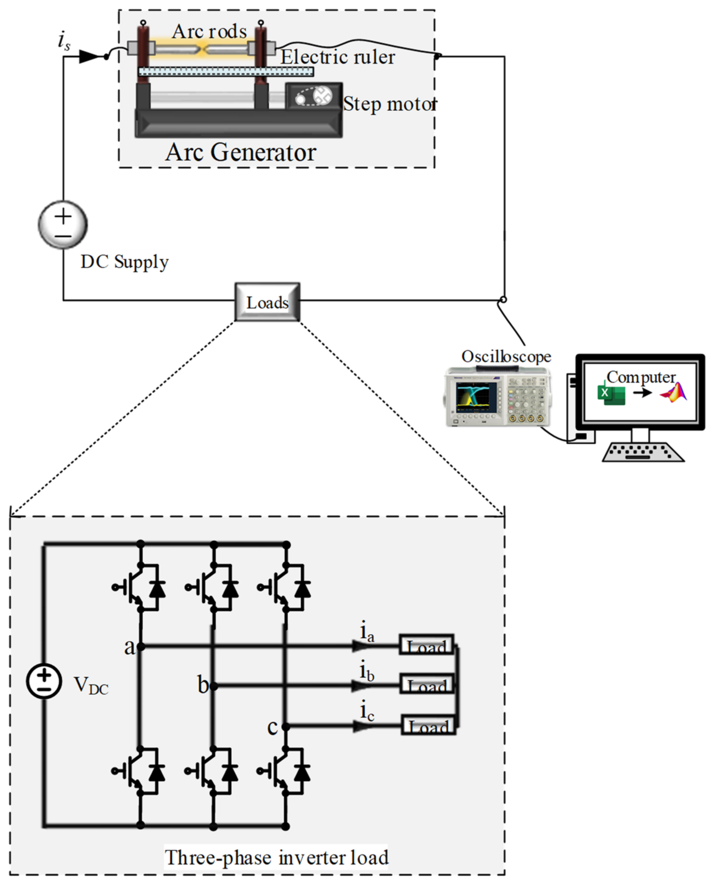
Figure 1 provides a detailed schematic representation of the process involved in acquiring DC arc data, following the guidelines stipulated in UL1699B (Underwriters Laboratories, Northbrook, IL, USA) [19]. The designed arc-generating circuit facilitated the creation of a series arc between the power source line and the load, as depicted in Figure 1. The controlled separation of the arc rods initiated the arc event, followed by the utilization of an oscilloscope to record the current waveforms passing through the rods both before and after the arcing incident. The Tektronix TCP312 current probe (Tektronix, Beaverton, OR, USA), capable of measuring frequency components from 0 to 100 MHz, was employed for accurate current measurement. Subsequent analysis of these arc currents was conducted using the MATLAB R2021b software (The Mathworks, Inc., Natick, MA, USA). The experimental setup for arc generation encompassed essential components, including a DC power supply, arc generator, and various loads. Notably, an N8741A DC power supply from Keysight Technologies, Santa Rosa, CA, USA, was employed, as illustrated in Figure 1. This power supply ensured precise control over the DC voltage supplied to the load. The separation of the arc rods was meticulously achieved by using a step motor mechanism, monitored by an electric ruler installed parallel to the rods. To ensure accurate data collection, an oscilloscope (Tektronix MSO3054, Beaverton, OR, USA) operating at a sampling frequency of 250 kHz was utilized. The precise measurement of arc current was facilitated using the Tektronix TCP312 current probe (Tektronix, Beaverton, OR, USA). The analysis of the DC arc faults encompassed both the temporal and spectral domains, and systematic DC arc generation was performed under various experimental conditions to enable comprehensive data collection. The specific experimental scenarios are outlined in

Table 1. Specifications of the arc fault experimental hardware.

Experimental Specifications	Supply Voltage	Switching Frequencies (${\mathit{f}}_{\mathit{s}\mathit{w}\mathit{i}}$)	Sampling Frequency (${\mathit{f}}_{\mathit{s}\mathit{a}\mathit{m}}$)	Current Amplitudes	Resistor Load	Inductor Load
Values	300 V	5, 10, 15, 20 kHz	250 kHz	5, 8 A	10 Ω	10 mH

for reference.

Figure 1 also presents the structural configurations of the three-phase inverter modules, which served as the primary load components in this research. The three-phase pulse width modulation (PWM) inverter, comprising SEMIKRON SKM50GB123D (SEMIKRON, Nuremberg, Germany) components with a 20 kW rating, supplied power to a three-phase load consisting of resistors and inductors. These inverters were responsible for converting the DC signals into AC signals, with only one switch within each phase leg active at any given time. This configuration resulted in eight distinct switching vectors, integral to the comprehensive functionality of the three-phase inverter system. Precise control over these inverter units was achieved using the implementation of space vector modulation (SVPWM), an advanced modulation technique known for its ability to finely regulate pulse width modulation. This control mechanism aimed to maintain a predetermined DC voltage while accurately manipulating the status of six individual switches, enabling the faithful replication of the sinusoidal waveforms typical of a three-phase AC system. This level of control ensured precise adjustments in both the frequency and amplitude parameters, thus guaranteeing accurate regulation throughout the experiments.

In this study, the control of these inverter units was adeptly executed by using the application of space vector modulation (SVPWM), an advanced modulation technique employed for precise control of pulse width modulation. The primary objective was to utilize a predetermined DC voltage and manipulate the status of six individual switches to accurately replicate the sinusoidal waveforms characteristic of a three-phase AC system. This control afforded the flexibility to finely tune both the frequency and amplitude parameters, ensuring precise regulation.

2.2. Characteristics of DC Arc Failure

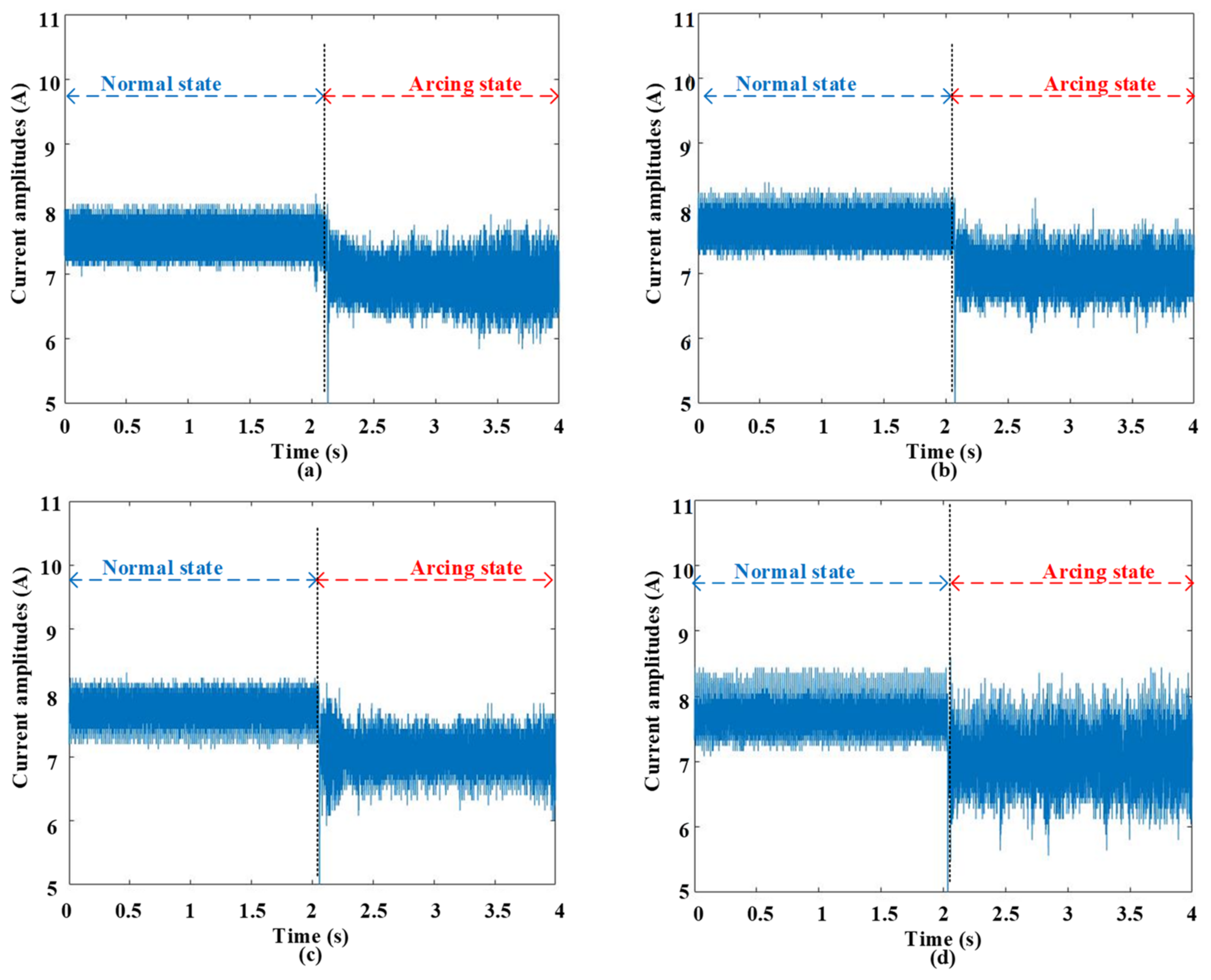
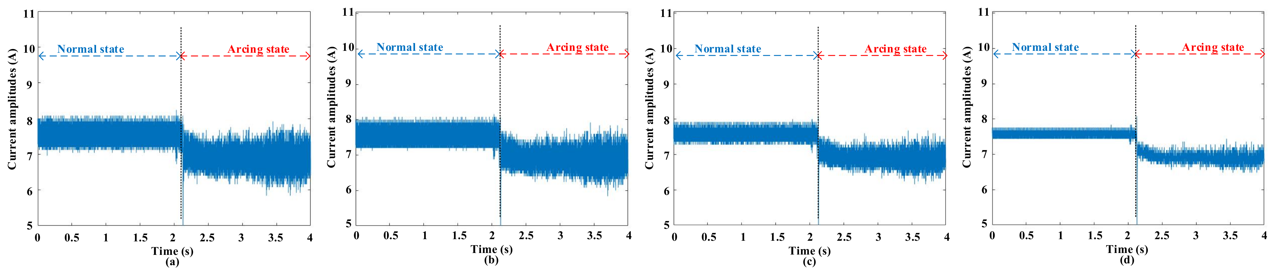
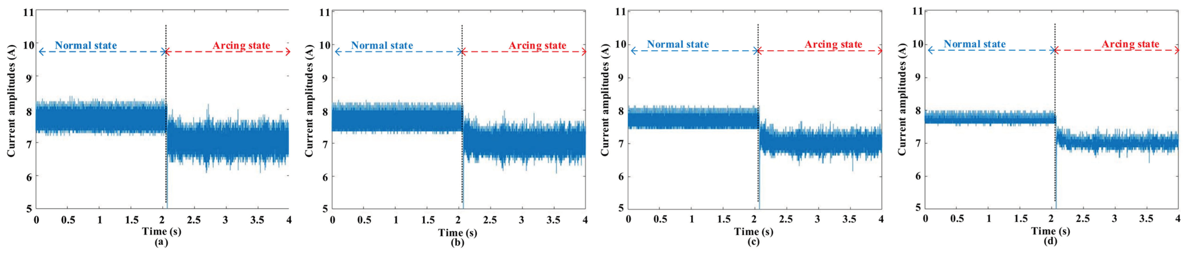
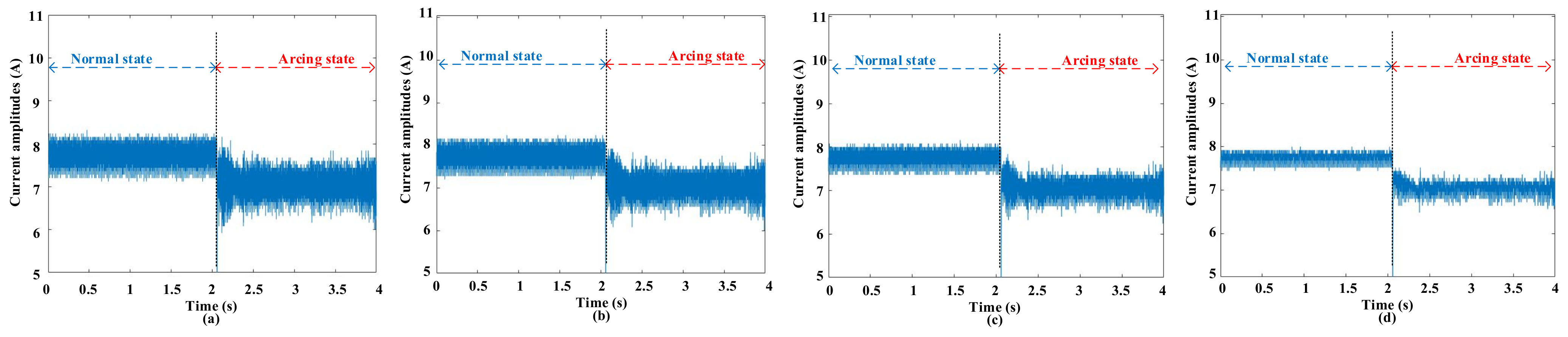
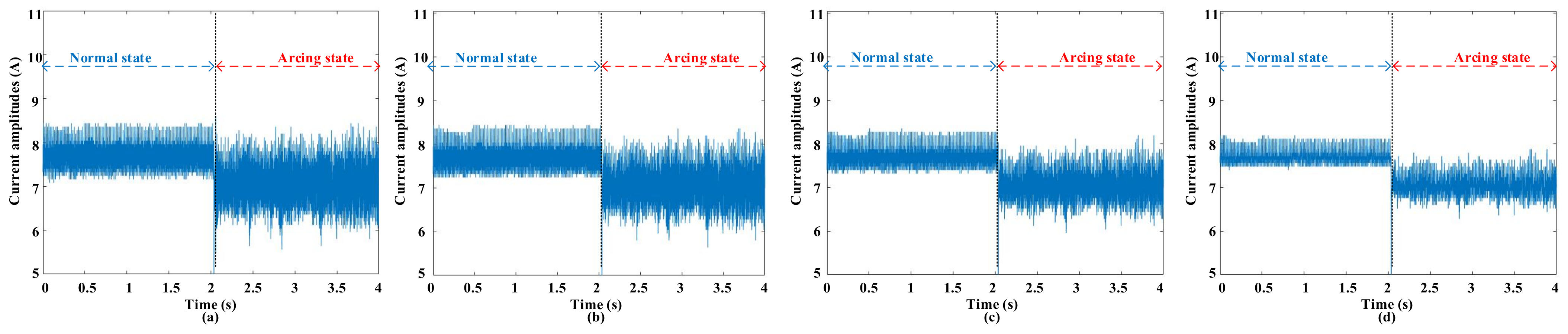
Figure 2 visually illustrates the waveforms corresponding to both normal and arcing states, recorded at different switching frequencies while maintaining a constant current amplitude of 8 A. Across the range of switching frequencies, the waveforms exhibit a consistent configuration before the onset of arcing. However, the emergence of an arc introduces a multitude of irregularities into these waveforms.

These anomalies include the introduction of harmonic components alongside the load current, resulting in a distortion of the load current waveform, as well as a slight reduction in current amplitude. The initial phase of arcing is distinctly characterized by prominent spikes in amplitude, a notable feature attributed to the electrical sparks generated during this phase. It is worth noting that the magnitude of these electrical sparks varies with the choice of switching frequencies. These pronounced deviations in the waveform behavior hold significant promise for utilization as discriminative features in the realm of arc fault detection.

3. Empirical Filtering Process and Artificial Intelligence Learning Algorithms

3.1. Empirical Rule

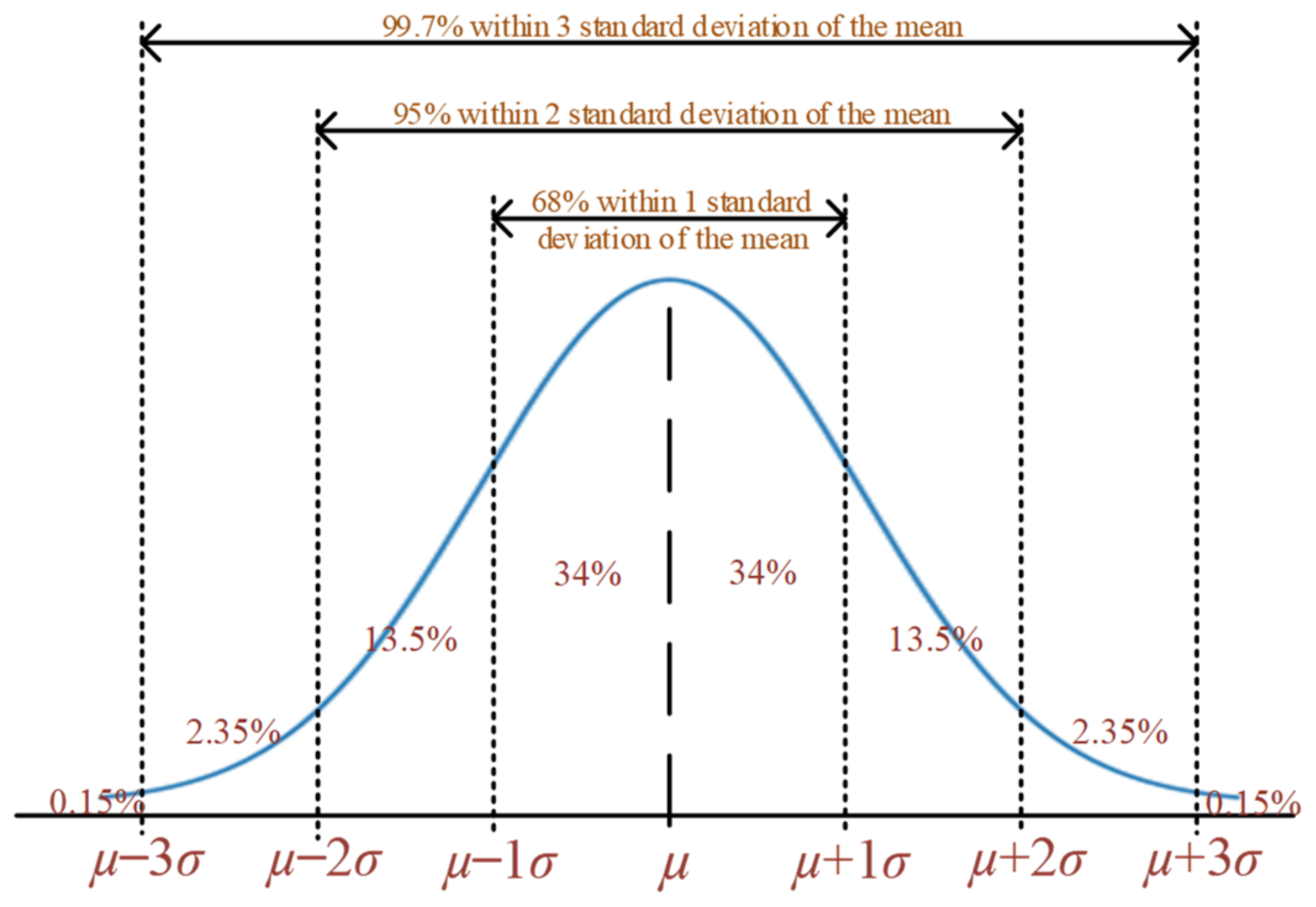
Analysts frequently employ the empirical rule to make predictions and assess the probabilities and distributions associated with the phenomena under investigation. This tool proves invaluable as it facilitates predictions based on easily calculable statistical metrics. An initial step involves confirming that the data align, at least approximately, with a normal distribution. In the realm of statistics, the empirical rule serves as a valuable asset for predicting eventual outcomes. Prior to the collection of precise data, it aids in generating rough estimates of the anticipated results. This is achieved using the calculation of standard deviations, enabling analysts to provide preliminary insights into the probable outcomes of forthcoming data collection and analysis endeavors.

This probability distribution, stemming from the empirical rule, assumes the role of an evaluative technique. It proves especially beneficial when acquiring precise data is a time-consuming or even unfeasible endeavor in certain scenarios. Such considerations come into prominence when organizations assess their quality control protocols or endeavor to gauge their exposure to various risks. The empirical rule, sometimes referred to as the three-sigma rule or the 68-95-99.7 rule, is a fundamental statistical guideline. It posits that in the context of data conforming to a normal distribution, nearly all observed data points cluster within three standard deviations (σ or std) of the mean (µ) [20]. As shown in Figure 3, the empirical rule is illustrated. It anticipates that within such distributions, approximately 68% of data points will reside within the range of the first standard deviation (µ ± σ), about 95% within the span of the first two standard deviations (µ ± 2σ), and an overwhelmingly vast majority of roughly 99.7% within the expanse of the first three standard deviations (µ ± 3σ) centered around the mean.

3.2. Filtering-Process-Based Empirical Rule

For any group of x, the mean (µ) and standard deviation (σ) could be obtained to find the probability density (pdf) of the variable taking on that group of x [21]. The formula of the normal probability distribution is expressed as:

$$pdf\left(x\right)=\frac{1}{\sigma \sqrt{2\pi }}{\epsilon }^{-\frac{{\left(x-\mu \right)}^2}{2{\sigma }^2}}$$

(1)

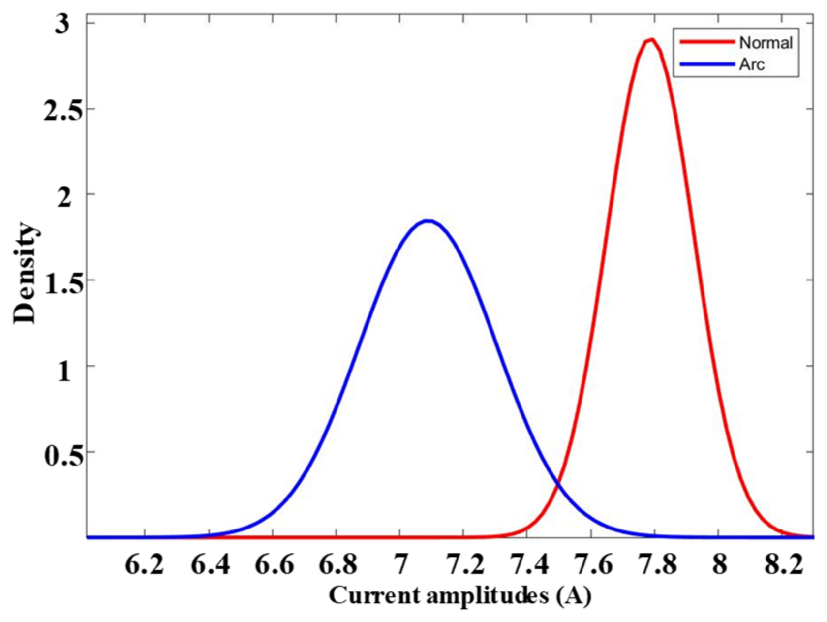
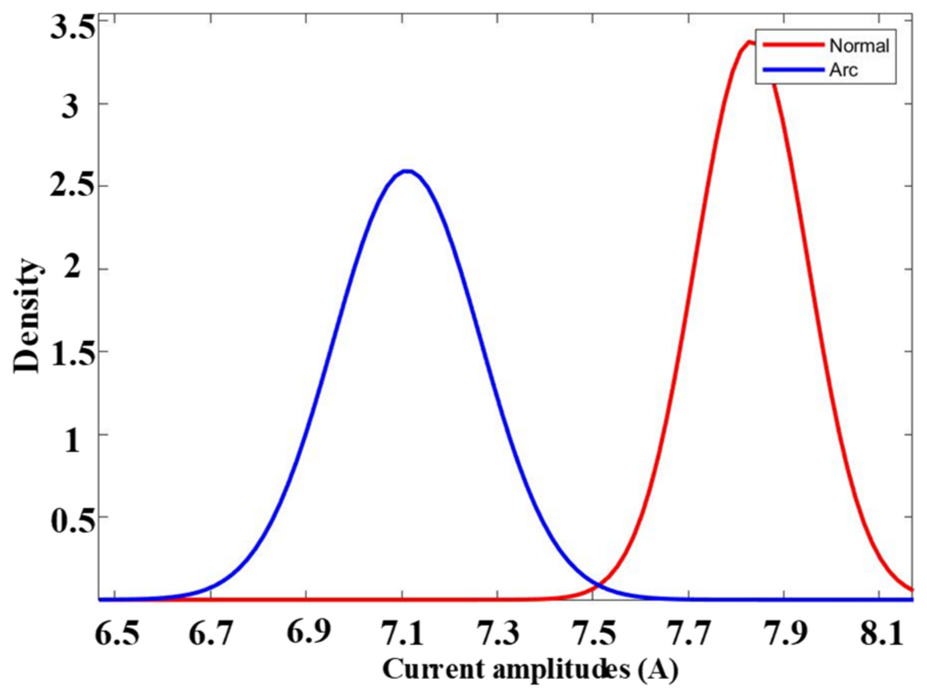
Figure 4 presents the probability distribution of the current for both normal and arcing states, focusing on scenarios with an 8 A current and a switching frequency of 10 kHz. This illustration involves the sampling of data over a duration of two seconds for both the stable normal and steady arcing states. Within each dataset, there are 200 data values, and the sampling frequency is set at 250 kHz, effectively capturing one second of data per set and accumulating a total of 1250 datasets for each state. Consequently, for the steady normal state and the steady arcing state, there are 1250 datasets, each containing 250,000 data values. This extensive dataset range for acquiring the normal distribution is substantially large, ensuring the fulfillment of the requirements for a normal distribution. On the other hand, the normal state current is primarily distributed between 7.4 A and 8.2 A, while the arcing state current is concentrated between 6.6 A and 7.6 A. This reveals an overlapping region between the normal and arcing states, potentially causing confusion when classifying these states directly. Utilizing such mixed data for classification can lead to reduced accuracy and erroneous predictions being made by the machine learning classifiers. To address this issue, an empirical filtering process is implemented to enhance classification accuracy.

The data, sampled at a frequency of 250 kHz, are segmented into smaller 0.8 ms datasets for filtering. Within each dataset, the mean and standard deviation are calculated, and the upper and lower limits are determined as

$$lower limit n=\mu \left(set\right)-n\times \sigma \left(set\right)$$

(2)

$$upper limit n=\mu \left(set\right)+n\times \sigma \left(set\right)$$

(3)

where n is 1, 2, or 3 and it represents the number of the standard deviation. Consequently, three distinct empirical filtering ranges are defined. Data falling within the specified range are retained, while data outside of the range are filtered out and replaced by the mean (µ).

Figure 5, Figure 6, Figure 7 and Figure 8 illustrate the current waveforms at 8 A and various switching frequencies before and after filtering using different filter ranges. When applying a filter with a three-standard-deviation range, only 0.3% of the data is filtered, resulting in minimal alteration to the waveform, which remains almost identical to the original signal. Conversely, the use of one and two standard deviation ranges produces noticeable dissimilarities between the filtered waveforms of the normal and arcing states, particularly with a one-standard-deviation range.

In comparison to alternative filtering methods, such as Xia et al.’s approach [22], which involves passing the signal through a bandpass filter ranging from 40 to 100 kHz and subsequently extracting the spectrum information using FFT, this method differs in some crucial aspects. Ref. [22] relied on a fixed threshold for arc fault identification, a limitation that can significantly constrain the algorithm’s adaptability. The issue arises because high-frequency components typically exhibit minute magnitudes, and variations in the specific conditions of solar PV stations can lead to different threshold requirements. In a similar vein, Wang and Balog’s study [8] delved into series arc current spectrum analysis using both discrete wavelet transform (DWT) and FFT. The DWT analysis offered insights into the spectrum variations over time, addressing a critical drawback of FFT, which fails to pinpoint the initiation time of the arc. However, the DWT approach, by decomposing the current signal into distinct frequency ranges, introduced increased complexity into the feature extraction process. In contrast, the proposed technique excels in detecting DC arcs by focusing on time–domain analysis of the arc currents subjected to empirical-rule-based filtering. This methodology balances complexity and robustness, enhancing the accuracy of arc detection.

Figure 9 provides a visual representation of the probability distribution of the current for steady normal and arcing states, emphasizing scenarios characterized by an 8 A current and a switching frequency of 10 kHz. The data depicted in this figure mirror that of Figure 4, capturing both the stable normal and arcing states, but with the added element of empirical filtering utilizing one standard deviation. This comparison reveals distinctive differences between the waveforms of normal and arcing states following empirical filtering, particularly within the one-standard-deviation range. These disparities in the filtered signals hold the potential to significantly enhance the efficacy of artificial intelligence learners (AILs) in accurately distinguishing between normal and arcing states.

3.3. Artificial Intelligence Learning Algorithms

The support vector machine (SVM) algorithm aims to identify an optimal hyperplane that effectively separates data points of one class from those of another class [23]. The K-nearest neighbor (KNN) algorithm operates on the premise that objects with similar attributes tend to be close neighbors, meaning similar entities cluster together [24]. In contrast, the decision tree (DT) methodology is versatile, serving for both classification and regression tasks. Its name reflects its tree-like structure, resembling a flowchart, which guides predictions based on a series of feature-driven divisions. The process begins at a root node and concludes with a decision at the terminal nodes [25]. Random forest (RF), as its name suggests, comprises an ensemble of individual decision trees. This collection of trees collaboratively contributes to making predictions. Each tree in the random forest generates a class prediction, and the class with the most votes determines the model’s prediction [26]. On the other hand, Naïve Bayes (NB) classifiers consist of a family of classification algorithms grounded in Bayes’ theorem. While not a single algorithm, these methods share a common principle: they assume independence between each pair of features being classified [27].

4. Intelligence Diagnosis of Series DC Arc Fault with Empirical Filtering

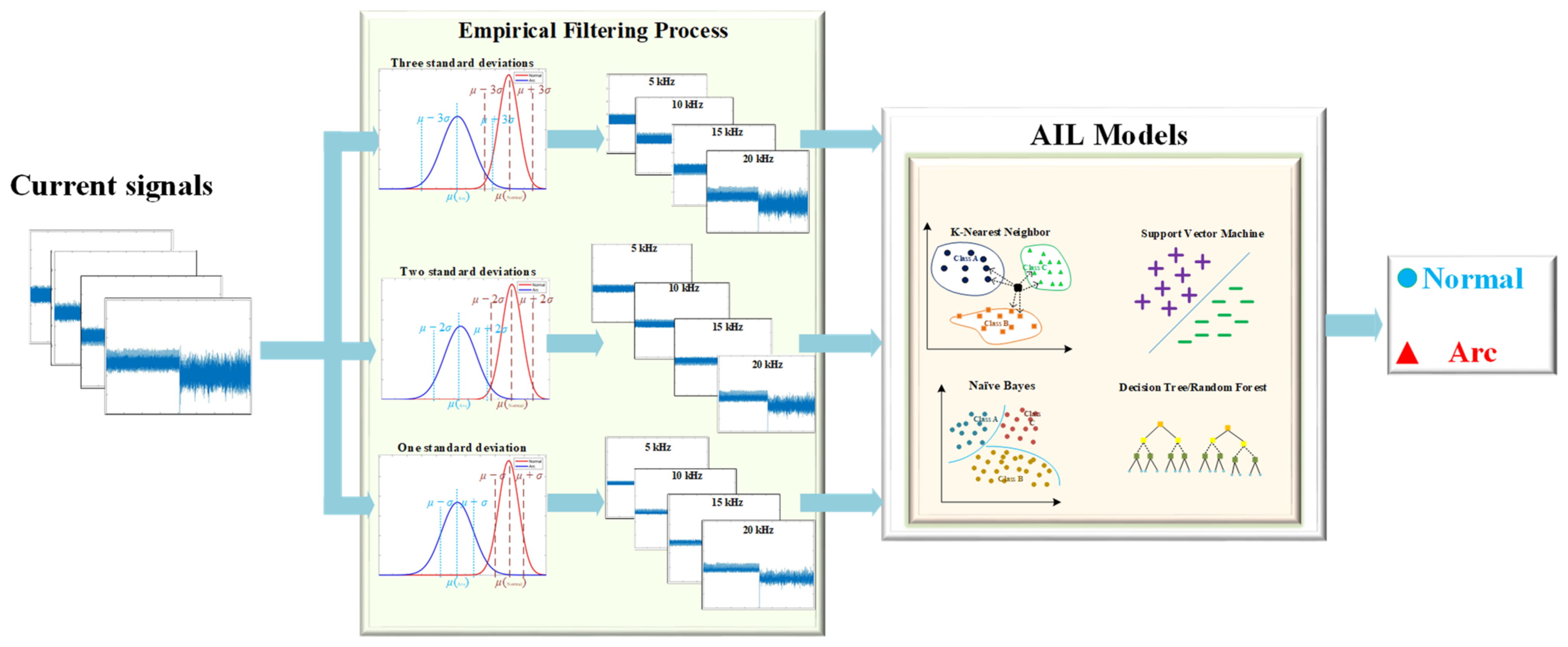
Figure 10 presents a schematic block diagram outlining the conceptual framework for the diagnosis of arc faults. The continuous current data undergo a precise sampling procedure and are subsequently partitioned into subdatasets, each containing 200 data points. These individual subsets of data then undergo a specialized filtering process, meticulously designed to remove data points that fall outside predefined ranges. To elucidate further, the data are initially sampled at a rapid rate of 250 kHz and segmented into smaller datasets, each with a duration of 0.8 ms, amounting to 200 data values per subset. Following this initial segmentation, the empirical filtering technique is meticulously applied, resulting in smoother and clearer signals. These refined signals subsequently serve as inputs for the AIL models within the context of DC arc fault diagnosis. It is important to note that the dataset encompasses two distinct current amplitudes, namely 5 A and 8 A, and four different switching frequencies, which include 5, 10, 15, and 20 kHz. Consequently, there are a total of eight distinct cases, with each case utilizing 3000 datasets for training and 1000 datasets for testing, resulting in a cumulative dataset of 24,000 for training and 8000 for testing. It is noteworthy that the distribution ratio between the normal and arc instances is meticulously maintained at a 1:1 proportion for both the training and testing phases. On the other hand, the ripple components increase with the increase in the switching frequency regardless of whether empirical filtering is employed or not, as shown in Figure 5, Figure 6, Figure 7 and Figure 8. It is noteworthy that the presence and magnitude of ripple components in the current signals could have a notable impact on the performance of the AIL models, especially at higher switching frequencies. Ripples introduce noise into the current signal. This noise may not be very significant at lower switching frequencies, but as the switching frequency increases, the amplitude of these ripples becomes more prominent. This can make it harder for AIL models to discern the underlying patterns in the data, as the ripples can mask the relevant information. The influence of ripple components can result in the AIL models making incorrect predictions or diagnoses, especially when the ripples coincide with the frequency ranges associated with fault signatures.

In the evaluation of AML algorithms, various metrics are employed as the primary criteria. The Accuracy detection rate, in particular, quantifies the proportion of correctly predicted datasets relative to the total number of test datasets. It is expressed as

$$\% of Accuracy=\frac{\# of correct predicted data set}{\# of total test data sets}.$$

(4)

The False Detection rate is calculated as the ratio of normal state datasets that are incorrectly predicted as the arcing state to the total number of normal state datasets. It is obtained as follows

$$\% of False Detection=\frac{\# of normal data sets predicted as arcing state}{total \# of normal data sets}.$$

(5)

Conversely, the Missing Detection rate is determined by the ratio of arcing state datasets that are inaccurately predicted as the normal state to the total number of arcing state datasets. It is determined as follows

$$\% of Missing Detection=\frac{\# of arcing datasets predicted as normal state}{total \# of arcing datasets}.$$

(6)

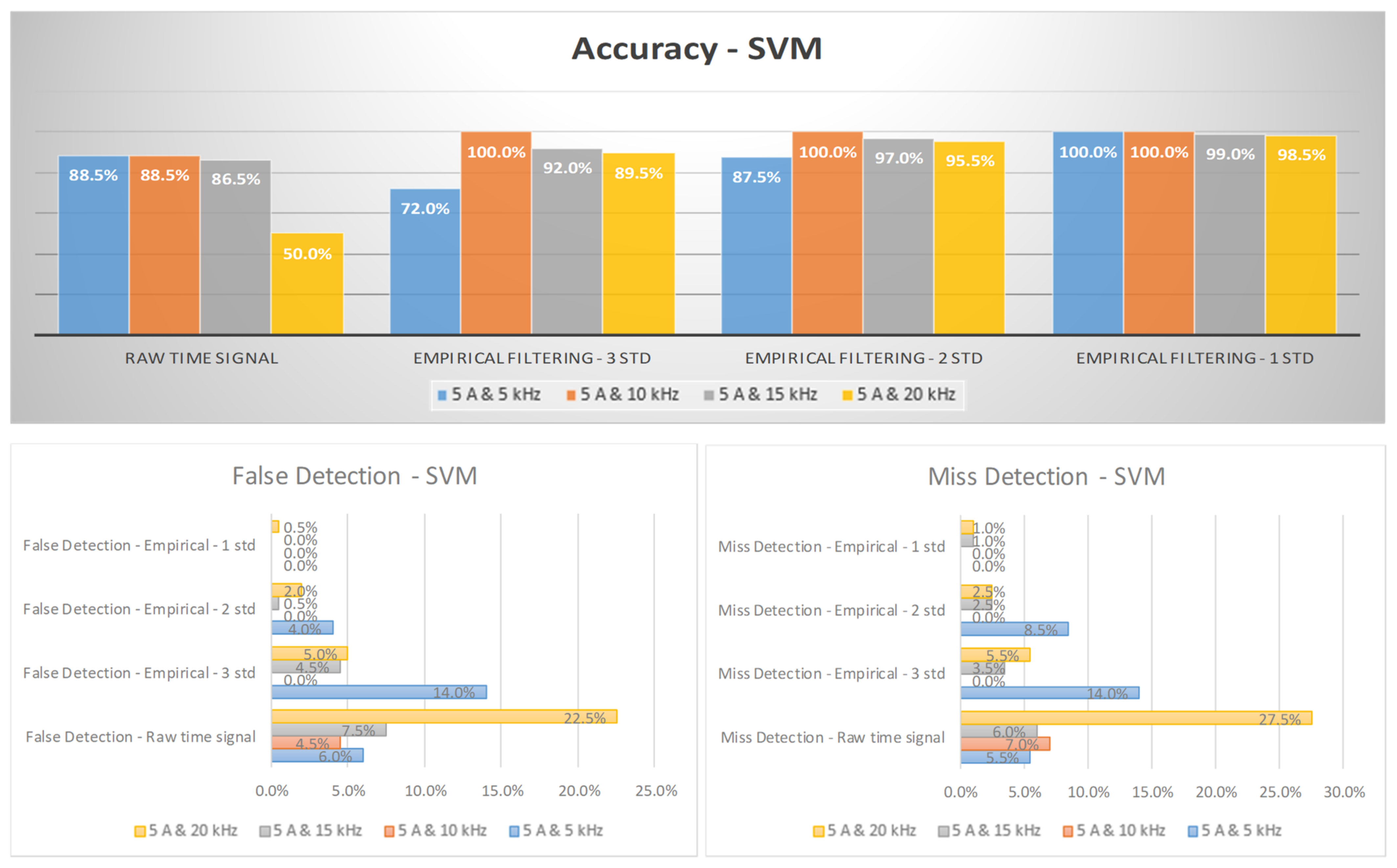
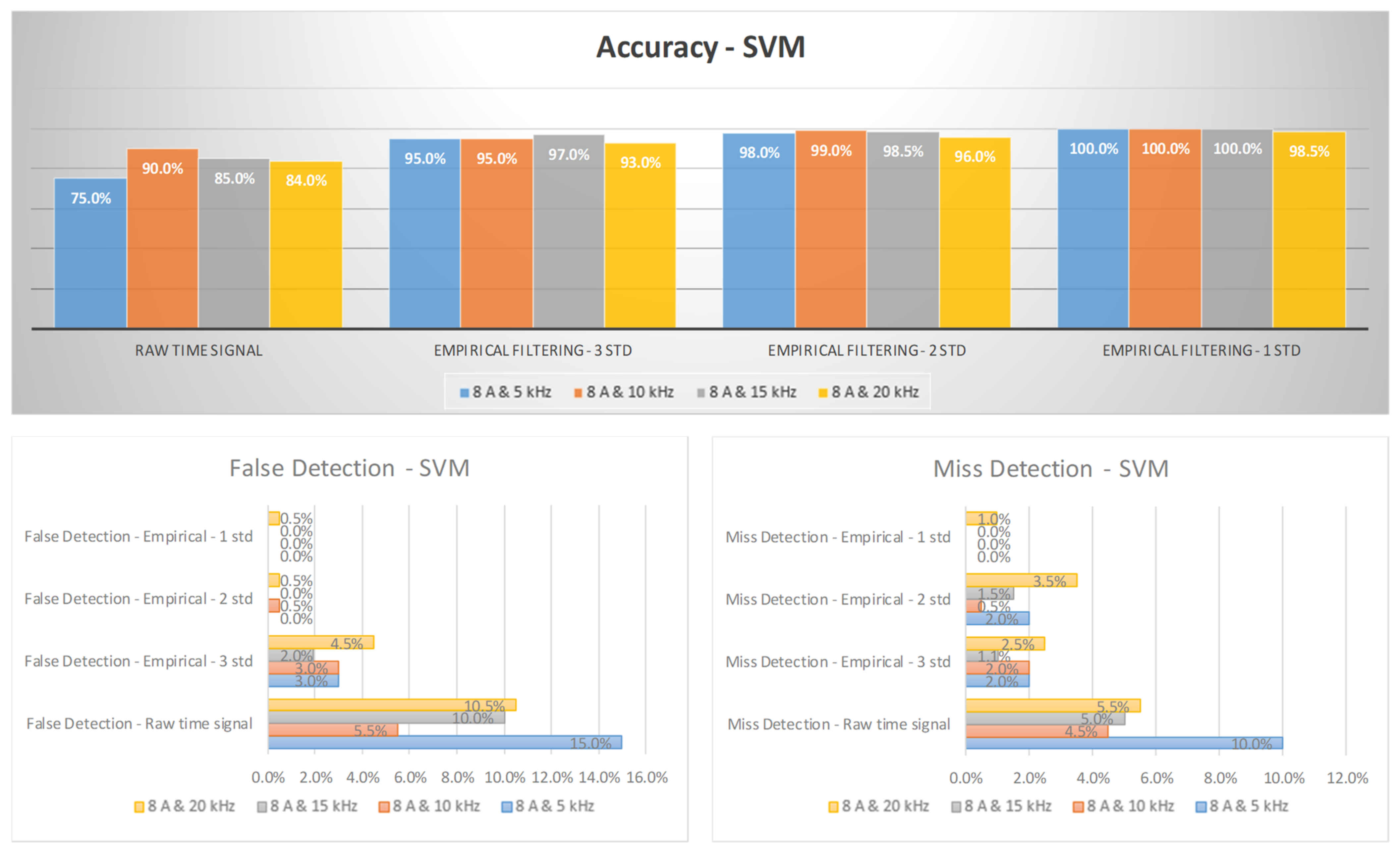
Figure 11 and Figure 12 depict the arc failure diagnosis rates for a three-phase inverter operating at 5 A and 8 A, respectively, across various switching frequencies. These rates are determined using empirical filtering and SVM. When the empirical filtering signals within the three σ ranges are utilized as inputs, there is a noticeable improvement in the accuracy of the fault detection compared to using the raw signals alone. Moreover, as the empirical filtering ranges are further refined to two and one σ ranges, the diagnosis rates for arc failure show additional enhancements. As elucidated in the filtering section, narrowing down the filtering ranges to two and one σ ranges renders the distinctions between normal and arcing states more discernible than the broader three σ range, thereby resulting in improved diagnosis accuracies. Furthermore, the adoption of the empirical filtering process concurrently leads to a reduction in false detection rates. This, in turn, mitigates false alarms, thereby bolstering the overall stability of the system. On the other hand, the diagnosis accuracies are highest at a 10 kHz switching frequency and gradually decrease with an increase in the switching frequency. The impact of ripple components is tied to the switching frequency and remains consistent, whether empirical filtering is utilized or not. While these ripples might be relatively inconspicuous at lower switching frequencies, their significance amplifies with increasing switching frequencies. As the switching frequency rises, so does the amplitude of these ripples. This heightened presence of ripples poses a notable challenge for AIL models. It complicates the task of uncovering the core data patterns since the ripples have the potential to overshadow the relevant information. This influence of ripple components can lead to inaccurate predictions or diagnoses being made by the AIL models, undermining their effectiveness in scenarios with higher switching frequencies.

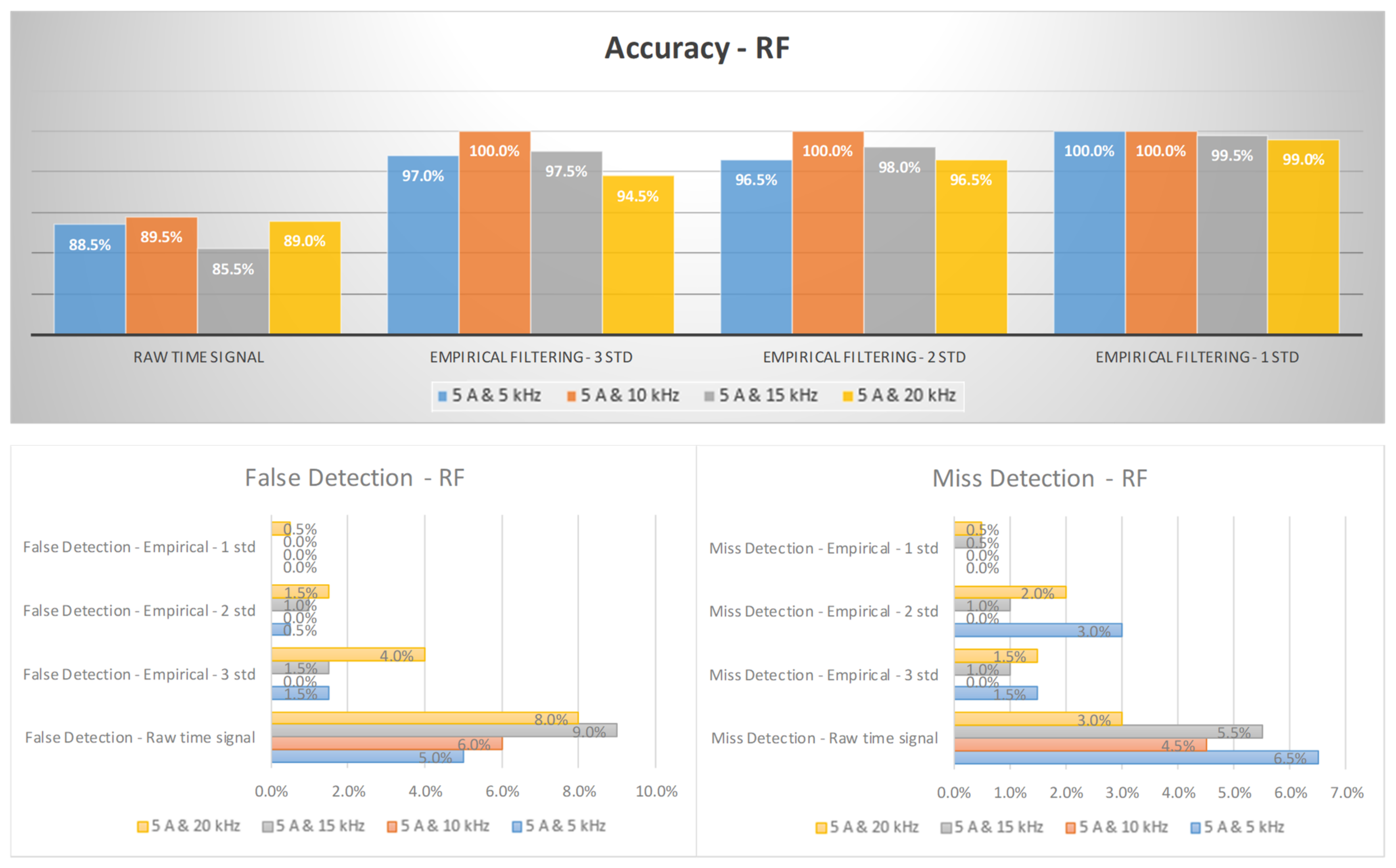
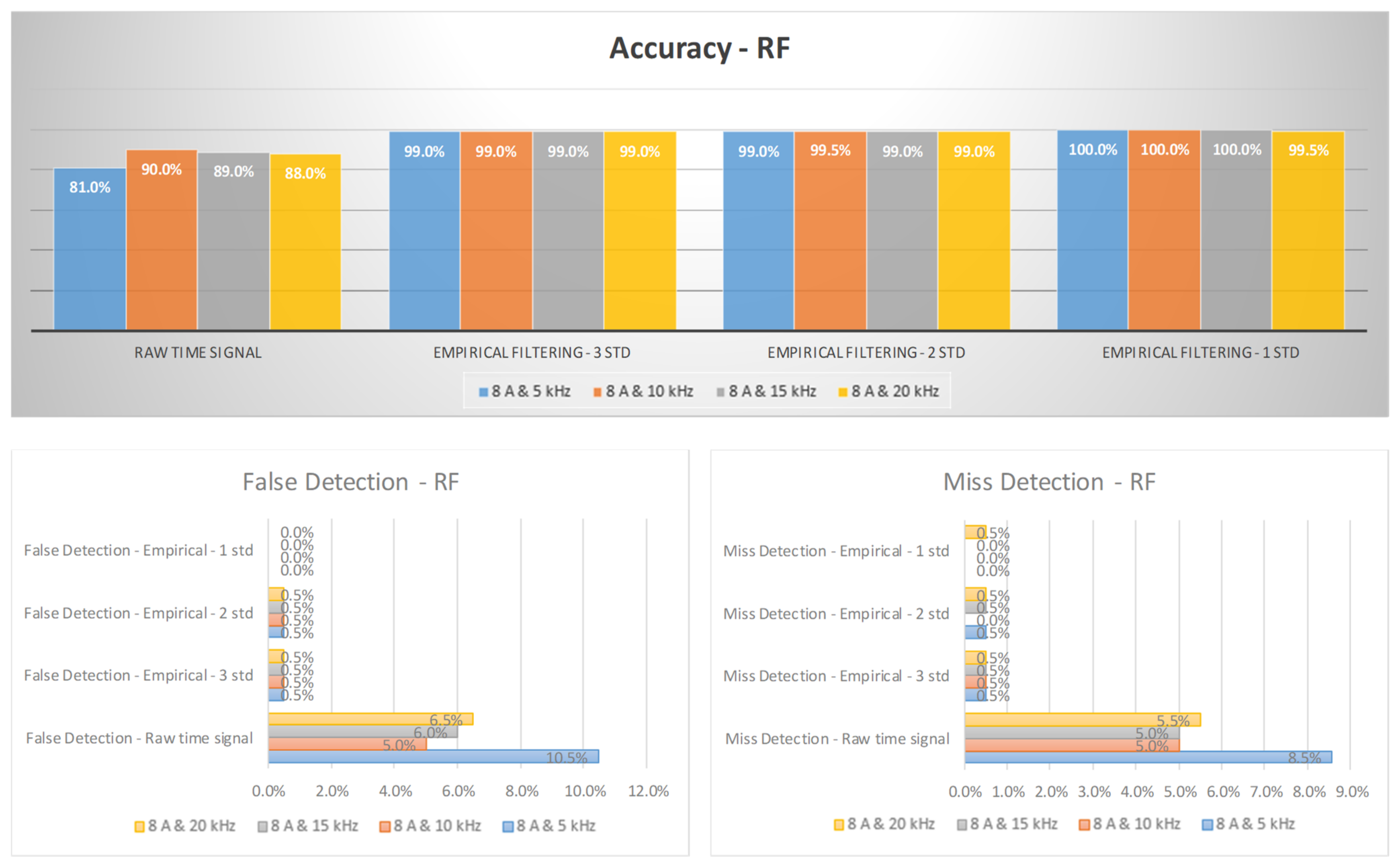
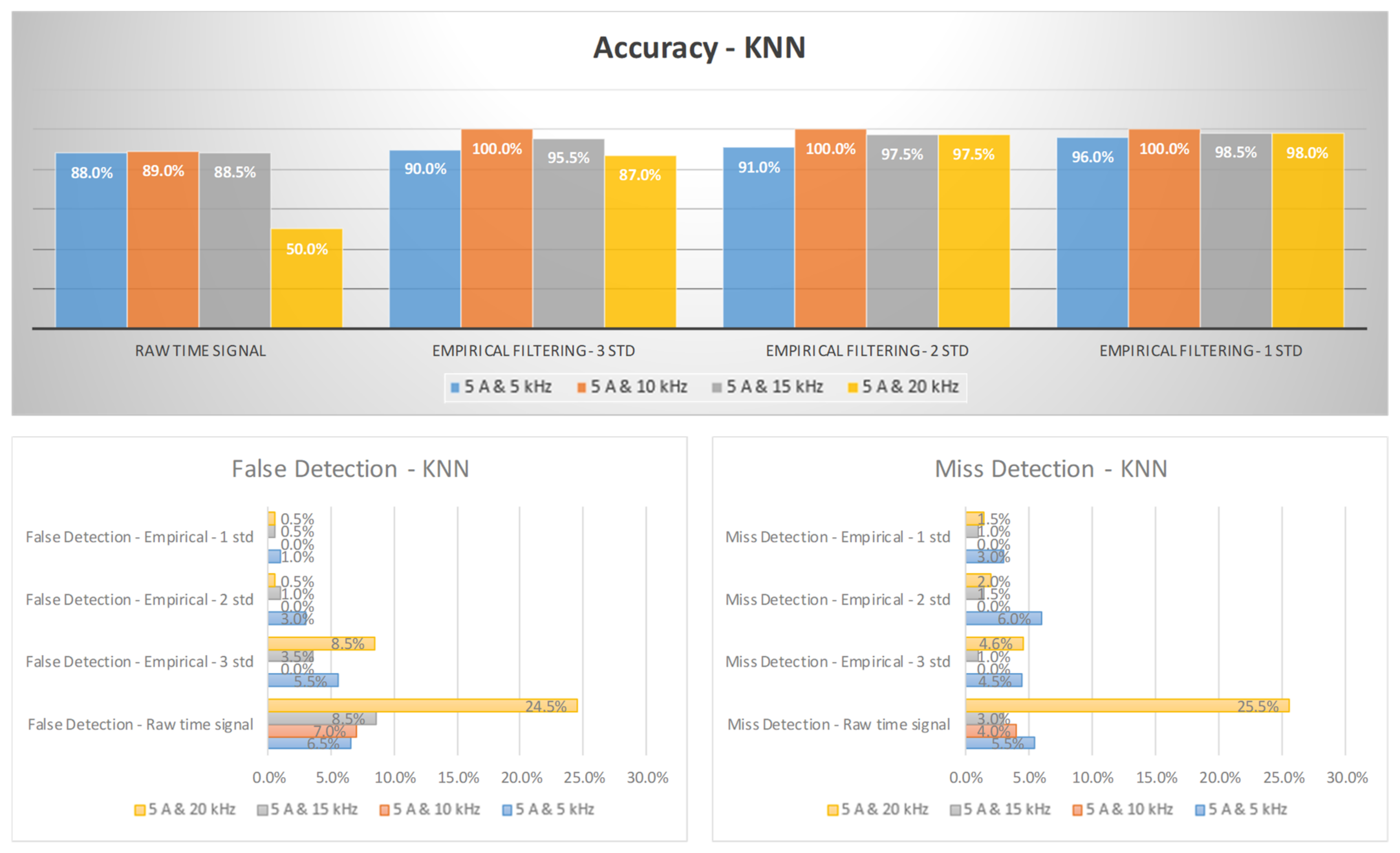
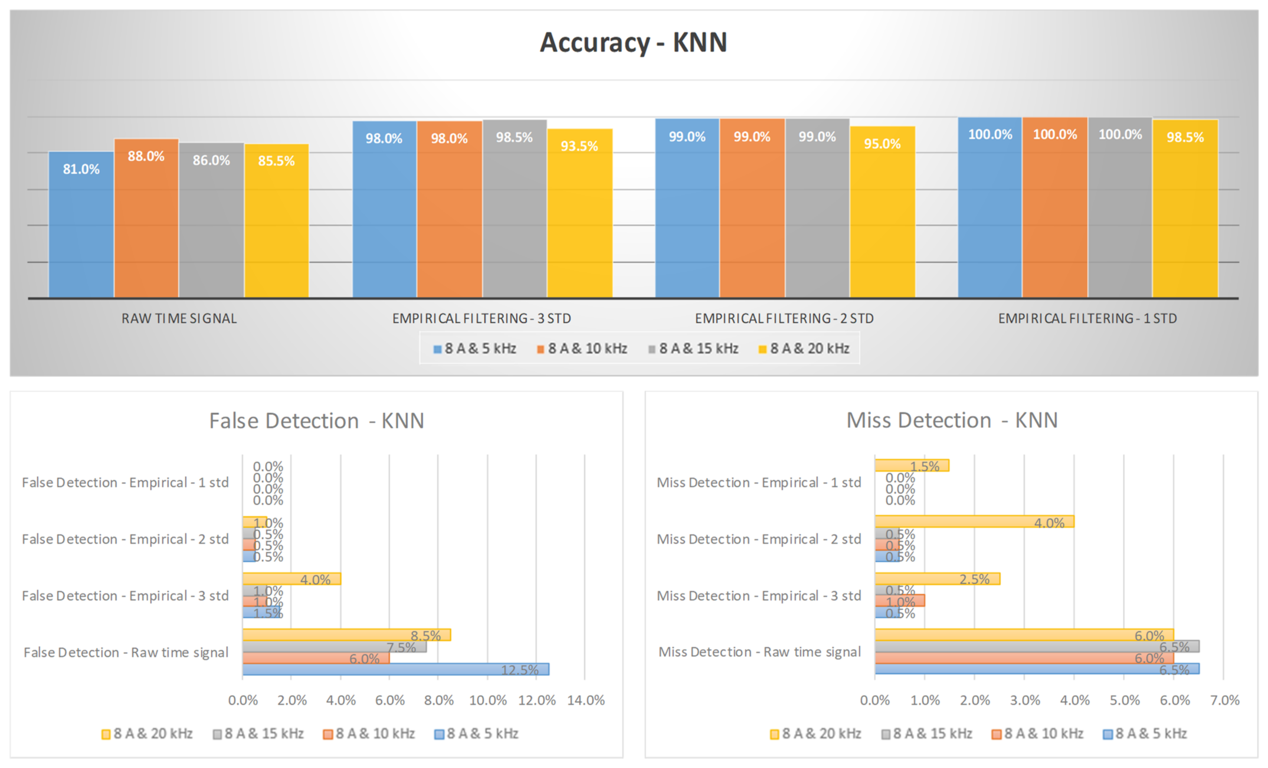
Figure 13 and Figure 14 illustrate the arc failure diagnosis rates for a three-phase inverter operating at 5 A and 8 A, respectively, across various switching frequencies. These rates are determined using empirical filtering in conjunction with an RF. The utilization of empirical filtering signals within the three σ ranges as inputs yields a discernible enhancement in the accuracy of arc fault detection when compared to relying solely on raw signals. Furthermore, as the empirical filtering ranges are further refined to two and one σ ranges, there are additional improvements in the diagnosis rates for arc failure. Figure 15 and Figure 16 illustrate the arc failure diagnosis rates for a three-phase inverter operating at 5 A and 8 A, respectively, across various switching frequencies. These rates are determined using empirical filtering in conjunction with the KNN algorithm. When the empirical filtering signals within the three σ ranges are utilized as inputs, a notable improvement in the accuracy of arc fault detection is observed compared to using the raw signals alone. Furthermore, as the empirical filtering ranges are further refined to two and one σ ranges, there are additional enhancements in the diagnosis rates for arc failure.

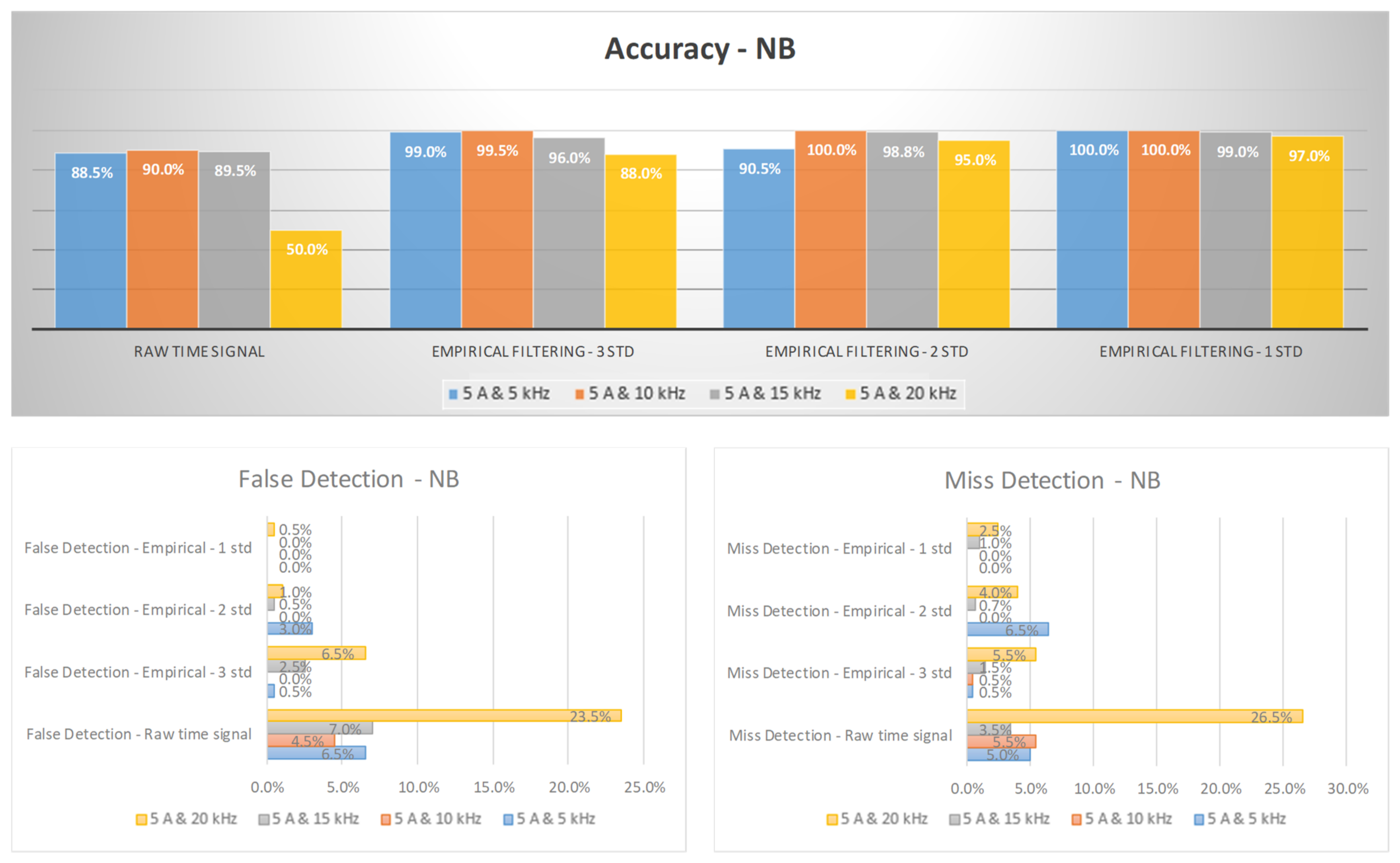
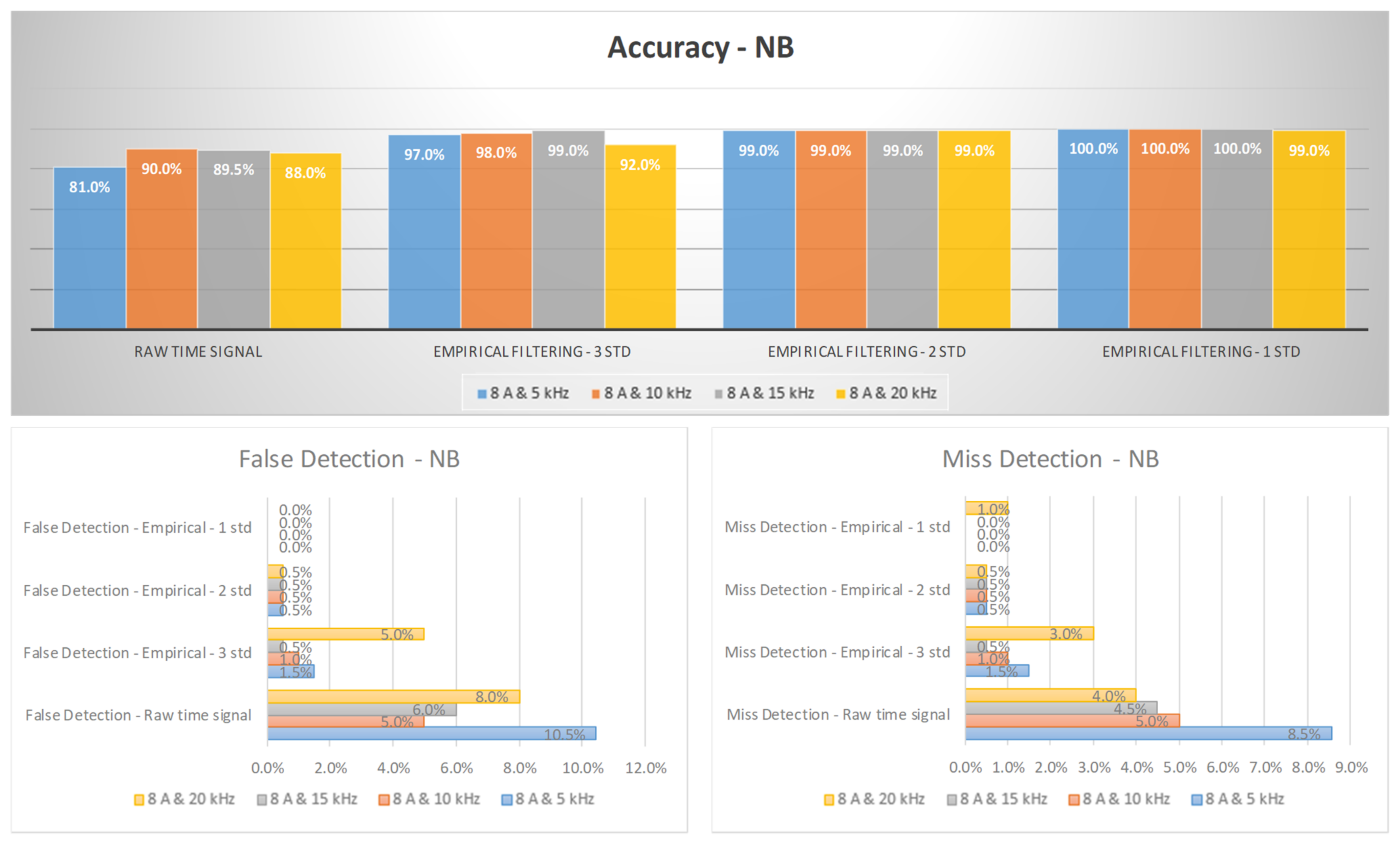
Figure 17 and Figure 18 provide a visual representation of the arc failure diagnosis rates for a three-phase inverter operating at 5 A and 8 A, respectively, across different switching frequencies. These rates have been computed by employing empirical filtering in tandem with the NB algorithm. Similarly to the mentioned AIL models, it is evident that when the empirical filtering signals within the three σ ranges are employed as inputs, a marked improvement in the accuracy of arc fault detection is discernible when compared to using the raw signals in isolation. Furthermore, as we further fine-tune the empirical filtering ranges to two and one σ ranges, we observe additional enhancements in the diagnosis rates for arc failure.

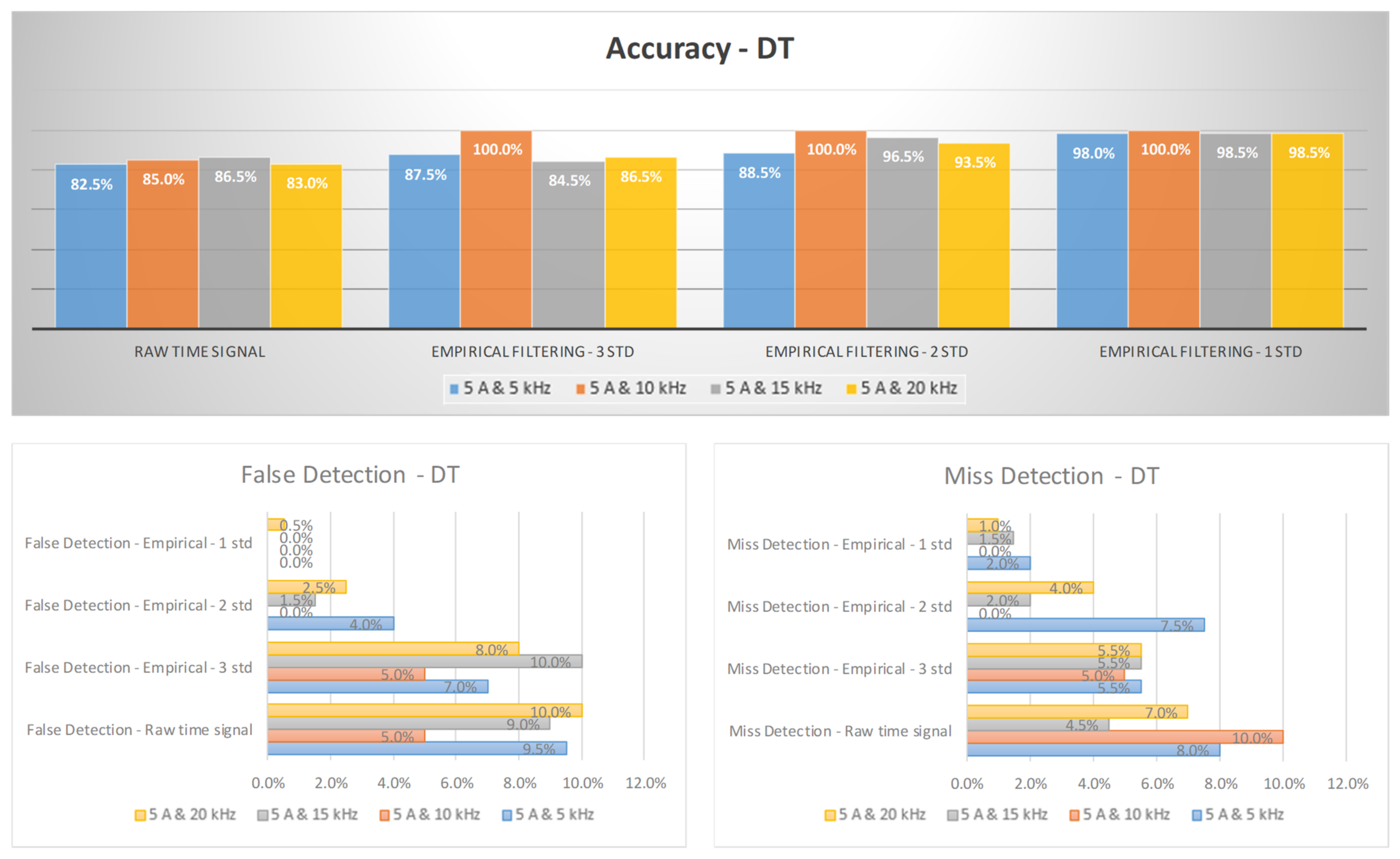
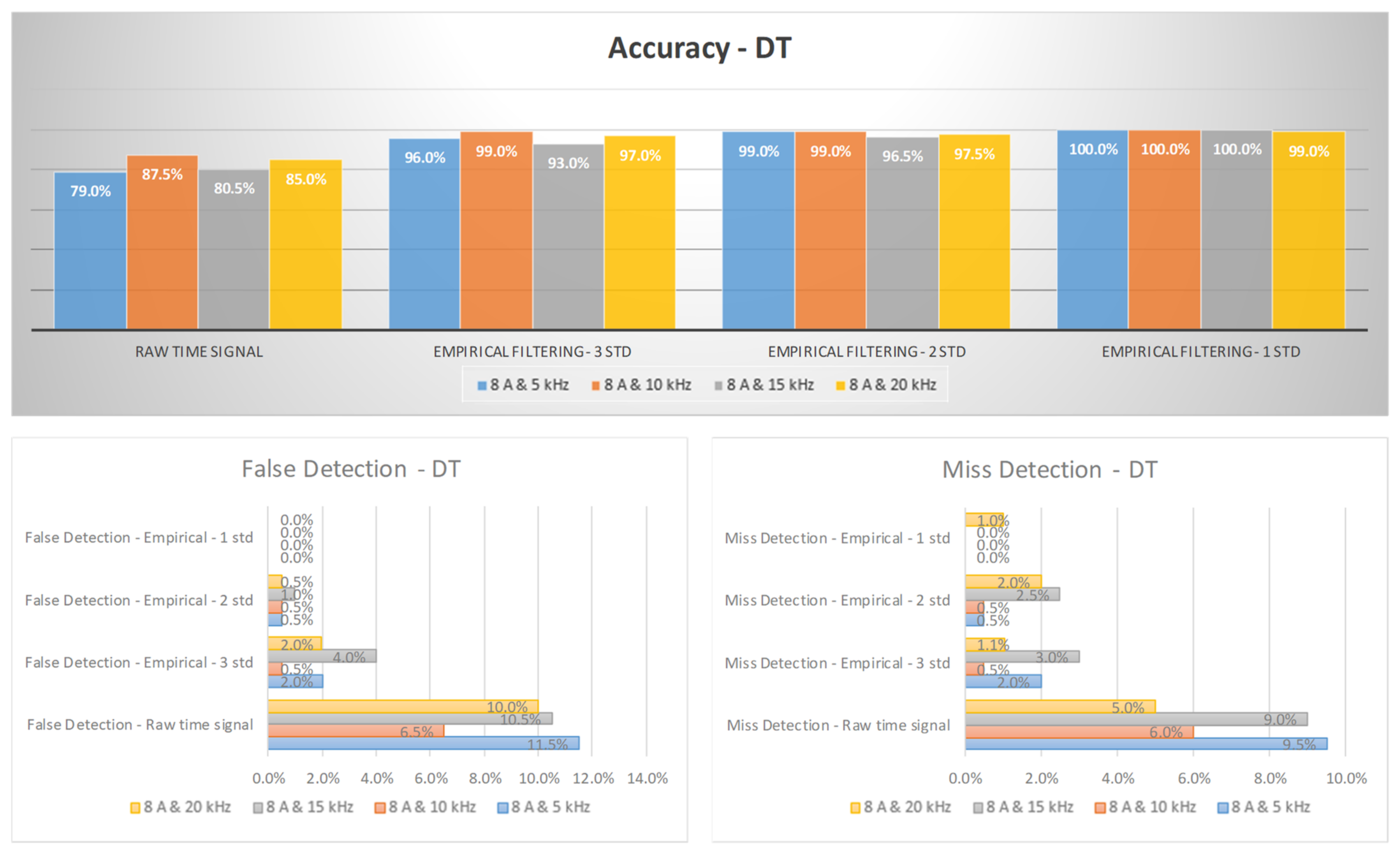
Figure 19 and Figure 20 provide a visual representation of the arc failure diagnosis rates for a three-phase inverter operating at 5 A and 8 A, respectively, across different switching frequencies. These rates have been computed using empirical filtering in tandem with the DT algorithm. It is evident that when the empirical filtering signals within the three σ ranges are employed as inputs, a marked improvement in the accuracy of arc fault detection is discernible when compared to using the raw signals in isolation. Furthermore, as we further fine-tune the empirical filtering ranges to two and one σ ranges, we observe additional enhancements in the diagnosis rates for arc failure.

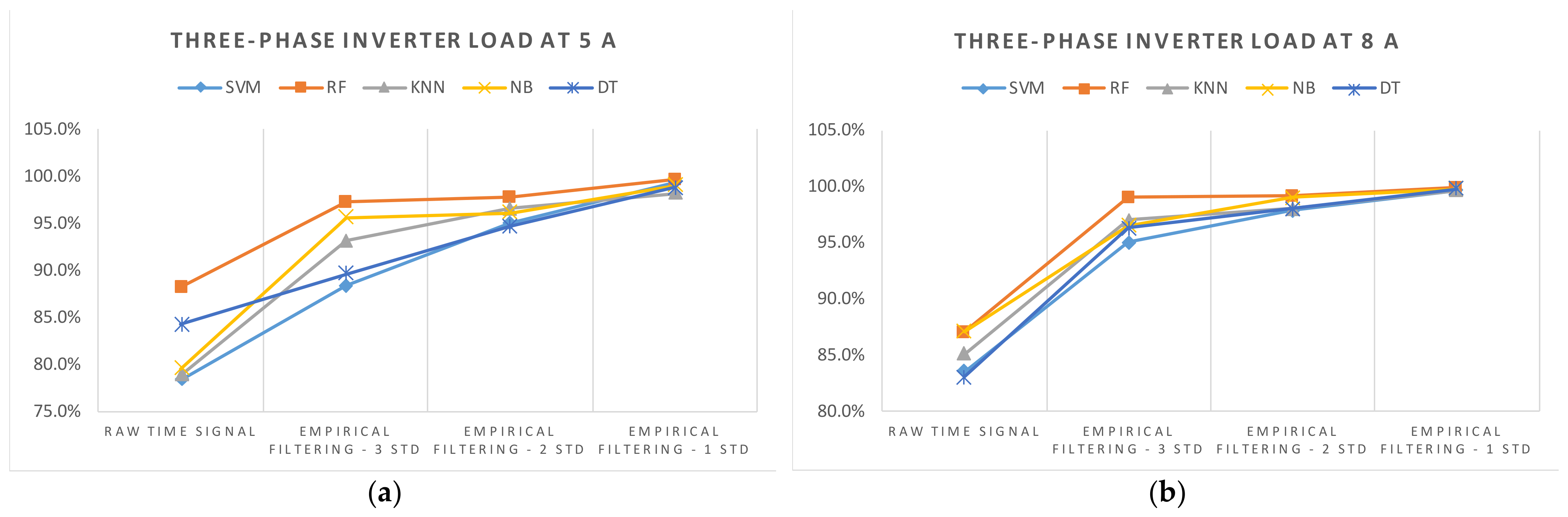
Figure 21 illustrates the comprehensive accuracy of the AIL models in detecting DC arc faults. Remarkably, among the inputs, the employment of empirical filtering with a one σ range yields the highest accuracies across all AIL models and switching frequencies. Notably, all the empirical filtering signals outperform the raw signals in terms of accuracy. Additionally, when considering the AIL models, an RF consistently emerges as the top-performing model, consistently achieving the highest diagnosis rates regardless of the inputs or switching frequencies. These diagnostic results unequivocally validate the efficacy of the proposed DC arc failure diagnosis scheme.

5. Conclusions

This research has successfully introduced an efficient and less complex diagnostic scheme for DC arc failure. The implementation of the empirical filtering procedure notably enhances signal clarity, resulting in more pronounced and distinct manifestations of arc distortions. This improvement in signal quality holds the potential to enhance the effectiveness of AIL models in arc diagnosis. The diagnostic results provide strong evidence for the efficiency of the proposed detection scheme. The analysis of the probability distribution of raw signals reveals an overlapping region between normal and arcing states, which can potentially lead to confusion when directly classifying these states. Using such mixed data for classification can reduce accuracy and result in incorrect predictions being made by machine learning classifiers. To address this issue, an empirical filtering process is applied to enhance the classification accuracy. By reducing this overlap, the empirical filtering technique significantly contributes to improved diagnostic performance. Furthermore, as the empirical filtering ranges are further refined to two and one σ ranges, the diagnosis rates for arc failure show additional improvements. Narrowing down the filtering ranges to two and one σ ranges makes the distinctions between normal and arcing states more discernible than the broader three σ range, leading to enhanced diagnosis accuracies. In addition, when considering AIL models, the RF consistently emerges as the top-performing model, achieving the highest diagnosis rates across various inputs and switching frequencies. The diagnostic evaluations conducted across all switching frequencies corroborate the effectiveness of the proposed arc detection scheme when integrated with the empirical filtering technique, notably enhancing the accuracy rates of all AIL models.

References

- Izquierdo, D.; Azcona, R.; Cerro, F.J.L.D.; Fernández, C.; Delicado, B. Electrical power distribution system (HV270DC), for application in more electric aircraft. In Proceedings of the 2010 Twenty-Fifth Annual IEEE Applied Power Electronics Conference and Exposition, Palm Springs, CA, USA, 21–25 February 2010; pp. 1300–1305. [Google Scholar]
- Herrera, L.; Zhang, W.; Wang, J. Stability analysis and controller design of DC microgrids with constant power loads. IEEE Trans. Smart Grid 2015, 8, 881–888. [Google Scholar]
- Alam, M.K.; Khan, F.; Johnson, J.; Flicker, J. A comprehensive review of catastrophic faults in PV arrays: Types detection and mitigation techniques. IEEE J. Photovolt. 2015, 5, 982–997. [Google Scholar] [CrossRef]
- Armijo, K.M.; Johnson, J.; Hibbs, M.; Fresquez, A. Characterizing fire danger from low-power photovoltaic arc-faults. In Proceedings of the 2014 IEEE 40th Photovoltaic Specialist Conference (PVSC), Denver, CO, USA, 8–13 June 2014; pp. 3384–3390. [Google Scholar]
- Pillai, D.S.; Rajasekar, N. A comprehensive review on protection challenges and fault diagnosis in PV systems. Renew. Sustain. Energy Rev. 2018, 91, 18–40. [Google Scholar] [CrossRef]
- He, C.; Mu, L.; Wang, Y. The detection of parallel arc fault in photovoltaic systems based on a mixed criterion. IEEE J. Photovolt. 2017, 7, 1717–1724. [Google Scholar] [CrossRef]
- Dhar, S.; Patnaik, R.K.; Dash, P.K. Fault detection and location of photovoltaic based DC microgrid using differential protection strategy. IEEE Trans. Smart Grid 2017, 9, 4303–4312. [Google Scholar] [CrossRef]
- Wang, Z.; Balog, R.S. Arc fault and flash signal analysis in DC distribution systems using wavelet transformation. IEEE Trans. Smart Grid 2015, 6, 1955–1963. [Google Scholar] [CrossRef]
- Vasile, C.; Ioana, C. Arc fault detection & localization by electromagnetic-acoustic remote sensing. In Proceedings of the IEEE Radio and Antenna Days of the Indian Ocean, Réunion Island, France, 10–13 October 2016; pp. 1–2. [Google Scholar]
- Ha, H.; Han, S.; Lee, J. Fault detection on transmission lines using a microphone array and an infrared thermal imaging camera. IEEE Trans. Instrum. Meas. 2011, 61, 267–275. [Google Scholar] [CrossRef]
- Zhao, S.; Wang, Y.; Niu, F.; Zhu, C.; Xu, Y.; Li, K. A series DC arc fault detection method based on steady pattern of high-frequency electromagnetic radiation. IEEE Trans. Plasma Sci. 2019, 47, 4370–4377. [Google Scholar] [CrossRef]
- Xiong, Q.; Ji, S.; Zhu, L.; Zhong, L.; Liu, Y. A novel DC arc fault detection method based on electromagnetic radiation signal. IEEE Trans. Plasma Sci. 2017, 45, 472–478. [Google Scholar] [CrossRef]
- Zhu, L.; Li, J.; Liu, Y.; Ji, S. Initial features of the unintended atmospheric pressure DC arcs and their application on the fault detection. IEEE Trans. Plasma Sci. 2017, 45, 742–748. [Google Scholar] [CrossRef]
- Balamurugan, R.; Al-Janahi, F.; Bouhali, O.; Shukri, S.; Abdulmawjood, K.; Balog, R.S. Fourier transform and short-Time fourier transform decomposition for photovoltaic Arc fault detection. In Proceedings of the 2020 47th IEEE Photovoltaic Specialists Conference (PVSC), Calgary, AB, Canada, 15 June–21 August 2020; pp. 2737–2742. [Google Scholar]
- Syafi’i, M.H.R.A.; Prasetyono, E.; Khafidli, M.K.; Anggriawan, D.O.; Tjahjono, A. Real time series DC Arc fault detection based on fast Fourier transform. In Proceedings of the 2018 International Electronics Symposium on Engineering Technology and Applications, Bali, Indonesia, 29–30 October 2018; pp. 25–30. [Google Scholar]
- Gu, J.; Lai, D.; Wang, J.; Huang, J.; Yang, M. Design of a DC series Arc fault detector for photovoltaic system protection. IEEE Trans. Ind. Appl. 2019, 55, 2464–2471. [Google Scholar] [CrossRef]
- Dang, H.-L.; Kwak, S.; Choi, S. Parallel DC Arc Failure Detecting Methods Based on Artificial Intelligent Techniques. IEEE Access 2022, 10, 26058–26067. [Google Scholar] [CrossRef]
- Dang, H.-L.; Kwak, S.; Choi, S. Identifying DC Series and Parallel Arcs Based on Deep Learning Algorithms. IEEE Access 2022, 10, 76386–76400. [Google Scholar] [CrossRef]
- UL 1699B; Outline of Investigation for Photovoltaic (PV) dc Arc-Fault Circuit Protection, Issue 2. Underwriters Laboratories, Inc.: Northbrook, IL, USA, 2013.
- Pukelsheim, F. The Three Sigma Rule. Am. Stat. 1994, 48, 88–91. [Google Scholar]
- Mehri-Dehnavi, H.; Agahi, H.; Mesiar, R. A New Nonlinear Choquet-Like Integral with Applications in Normal Distributions Based on Monotone Measures. IEEE Trans. Fuzzy Syst. 2019, 28, 288–293. [Google Scholar] [CrossRef]
- Xia, K.; He, Z.; Yuan, Y.; Wang, Y.; Xu, P. An arc fault detection system for the household photovoltaic inverter according to the DC bus currents. In Proceedings of the 2015 18th International Conference on Electrical Machines and Systems (ICEMS), Pattaya, Thailand, 25–28 October 2015; pp. 1687–1690. [Google Scholar]
- Boser, B.E.; Guyon, I.M.; Vapnik, V.N. A training algorithm for optimal margin classifiers. In Proceedings of the Fifth Annual Workshop on Computational Learning Theory, (COLT′92), Pittsburgh, PA, USA, 27–29 July 1992; pp. 144–152. [Google Scholar]
- Cover, T.; Hart, P. Nearest neighbor pattern classification. IEEE Trans. Inf. Theory 1967, 13, 21–27. [Google Scholar] [CrossRef]
- Breiman, L.; Friedman, J.; Olshen, R.; Stone, C. Classification and Regression Trees; Statistics/Probability Series; Wadsworth and Brooks: Belmont, CA, USA, 1984. [Google Scholar]
- Breiman, L.; Learn, M. Random forests. Mach. Learn. 2001, 45, 5–32. [Google Scholar] [CrossRef]
- Langley, P.; Iba, W.; Thompson, K. An analysis of Bayesian classifiers. In Proceedings of the Tenth National Conference on Artificial Intelligence, San Jose, CA, USA, 12–16 July 1992; pp. 223–228. [Google Scholar]
Figure 1.
DC arc fault experimental setup. a, b, and c are the names of three-phase of inverter.
Figure 2.
Current signals for different switching frequencies at 8 A current amplitude. (a) 5 kHz. (b) 10 kHz. (c) 15 kHz. (d) 20 kHz.