A New Automated Classification Framework for Gear Fault Diagnosis Using Fourier–Bessel Domain-Based Empirical Wavelet Transform

Abstract

Gears are the most important parts of a rotary system, and they are used for mechanical power transmission. The health monitoring of such a system is needed to observe its effective and reliable working. An approach that is based on vibration is typically utilized while carrying out fault diagnostics on a gearbox. Using the Fourier–Bessel series expansion (FBSE) as the basis for an empirical wavelet transform (EWT), a novel automated technique has been proposed in this paper, with a combination of these two approaches, i.e., FBSE-EWT. To improve the frequency resolution, the current empirical wavelet transform will be reformed utilizing the FBSE technique. The proposed novel method includes the decomposition of different levels of gear crack vibration signals into narrow-band components (NBCs) or sub-bands. The Kruskal–Wallis test is utilized to choose the features that are statistically significant in order to separate them from the sub-bands. Three classifiers are used for fault classification, i.e., random forest, J48 decision tree classifiers, and multilayer perceptron function classifier. A comparative study has been performed between the existing EWT and the proposed novel methodology. It has been observed that the FBSE-EWT with a random forest classifier shows a better gear fault detection performance compared to the existing EWT.

1. Introduction

Gearbox fault diagnosis is the process of analyzing the health and performance of gears in machinery to detect potential faults or issues before they become major problems. It involves using techniques like vibration analysis, oil analysis, acoustic emission testing, and thermography to identify and diagnose gear conditions. S. Sheng [1] proposed some first-hand oil and wear debris analysis based on the testing of full-scale wind turbine gearboxes. T. Nowakowski et al. [2] proposed a system for monitoring the condition of tram gearboxes that is based on trackside acoustic data. Infrared thermography for a condition monitoring tool was described in S. Bagavathiappan et al. [3] as a method that does not involve physical touch and can be used to monitor the temperatures of things or processes in real time. Gearbox fault diagnosis is essential for minimizing downtime, reducing the risk of catastrophic failures, and extending the lifespan of gears, ensuring the safety, the reduction in maintenance costs, and the reliable operation of machines and systems which rely on gears [4]. Several different factors might cause a gear to fail, including fatigue, impact, wear, or plastic deformation. The most common cause of failure in gearing is fatigue. When a fault is going to propagate, the system generates noise and vibration. Further down the line, gear failure occurs due to the excessive vibration. When it comes to monitoring the status of machines during startups, breakdowns, and regular operations [5], vibration measuring is a technology that is successful, discrete, adaptable, and cost-effective. Furthermore, article [6] provides a detailed evaluation or selection of signal processing techniques that have been applied to try to minimize the amount of noise that exists in the vibration signals, as well as to isolate and emphasize the elements of the signals that are connected to faults in order to accomplish the goal of reliable fault identification. Considering the basics of various signal processing approaches, these methods are capable of being divided into three distinct groups. Analysis in the time domain, analysis in the frequency domain, and analysis in the time–frequency domain are the three basic types of methodologies that are employed in vibration analysis. The fact that nonstationary or variable-in-time signals are amplitude- and frequency-modulated means that the time domain and frequency domain methods cannot be used to analyze these types of signals. In real-world circumstances, the operation of a gearbox leads to the generation of nonstationary signals due to vibration [7]. Vibration analysis is an effective tool for diagnosing such signals. For local gear faults such as the levels of a gear tooth crack [8], identification is needed to prevent any unanticipated gear failure because of the tooth breakage of gear initiates due to an incipient crack in the gear [9,10]. Severe vibration is one of the key contributing variables that might lead to an investigation into a local defect in a gearbox [11]. This investigation might be necessary because of the severity of the vibration. The evaluation of nonstationary signals frequently makes use of time–frequency domain analysis techniques such as the short-time Fourier transform (STFT), the continuous wavelet transform (CWT), the discrete wavelet transform (DWT), the Tunable-Q wavelet transform (TQWT), the Hilbert–Huang transform (HHT), the Wigner–Ville distribution (WVD), the empirical mode decomposition (EMD), the wavelet packet transform (WPT), and the variational mode decomposition (VMD) [12,13,14,15,16,17,18,19,20]. Because STFT uses a fixed-moving window, a time–frequency (TF) multiresolution analysis was not feasible with this technique. In order to work around this limitation, WT offers a useful representation of nonstationary signals that may be used with the TF domain. Morlet et al. introduced the wavelet transform (WT) in the 1980s [21]. Wavelet analysis is a TF analysis technique that can provide high-resolution time–frequency representations of nonstationary signals such as sound and vibration signals [21]. Saravanan et al. [15] employed an ANN and proximal support vector machines (PSVM) to diagnose a malfunction in a bevel gearbox using features derived from the CWT wavelet. Syed et al. [22] applied the DWT with the mean square energy to demonstrate outstanding defect diagnostic qualities using different classifiers and, as a result, it is strongly encouraged. Upadhyay et al. [14] presented a new technique based on tunable Q-wavelet transform and fractal-based features for the diagnosis of bearing defects. WT struggles with the dilemma of which mother wavelet to use and how many decomposition levels to use [23]. The WVD, on the other hand, offers a better time–frequency resolution; however, it does contain a few cross-terms [23]. For the investigation of nonstationary signals, Gilles [24] developed an innovative constructing approach called the empirical wavelet transform (EWT). The authors [25] conducted more research on the EWT method to determine its applicability with multivariate signals; also, they presented a multivariate TF formulation that was based on the EWT method. The EWT performs substantially better than the ensemble empirical mode decomposition (EEMD) and EMD techniques when it comes to the estimating mode, and it also greatly cuts down the amount of time needed for computation [26]. EWT is a method of adaptive decomposition that eliminates narrow-band frequency bands within the examined signal depending on the frequency details of the spectrum. After locating the boundary frequencies in the FT-based spectrum, it next applies adaptive wavelet-based filters to the signals in order to deconstruct them [25]. However, EWT is unable to accurately depict frequency components that are tightly spaced. Challenges similar to those experienced with the EWT approach have been found in the suggested method. A limited amount of work has been reported for the fault detection of gear considering EWT. Anupam et al. [27] applied the EWT technique over polymer gear to detect faults, but they have not worked on enhancing the EWT performance with a combination of other filter methods such as FBSE. In this study, the established EWT procedure is revised using the FBSE. It has been noted that the nonstationary class of the Bessel function is based on the FBSE in nature [25]. Further, it is what makes the FBSE coefficients effective for the spectrum analysis of such signals. Although, FBSE-EWT was mostly employed in biological signals like vectorcardiogram signals, electroencephalography (EEG) signals, etc. [25]. Researchers used the multifrequency scale-based two-dimensional FBSE-EWT method for glaucoma detection, which requires the segmentation of fundus photographs into sub-images. This method proposes a rhythm separation technique and enhanced local polynomial (LP) approximation-based total variation (TV) for the filtering of ocular artefacts from the EEG signals. The FBSE-EWT technique is not used to investigate gear faults like chipped teeth, missing teeth, cracks in the root, and worn gear faces with classifiers. As a result, FBSE-EWT has been applied in this research to identify the gear crack faults at various levels and compare their performance with EWT.

Correct feature selection is necessitated by pattern recognition and the gathering of knowledge-based data. Statistically based characteristics have been shown to successfully detect bevel gear vibration signals in signal analysis in refs. [15,28]. Therefore, this work employed the use of statistical characteristics such as kurtosis, variance, root mean square, and Shannon entropy to draw out relevant information. The Kruskal–Wallis test is applied to determine whether or not the statistical result is significant; hence, features extracted from a group of samples may be utilized as a classification input parameter. Nonstationary properties of a signal, such as a change in frequency throughout an operation, provide an unacceptable circumstance for gear vibration signals [29]. Therefore, it is extremely difficult to analyze such signals when they are flawed. Machine-learning-based defect detection is advantageous in this situation [29,30,31]. Researchers have made extensive use of classifiers over the past decade to increase the effectiveness of applicable signal-processing algorithms for fault identification. Artificial neural networks (ANN), linear discriminant analysis (LDA), support vector machines (SVM), genetic algorithms (GA), K-nearest neighbor (KNN), fuzzy logic, Bayesian networks, and decision trees are some of the machine learning approaches that can be used as classification tools for low fault identification and gearbox condition monitoring [15,27,28,29,32,33]. The ANN technique is based on learning to recognize patterns. But it may lead to overfitting the dataset, which is undesirable. When it comes to minimizing risk, SVM misses the mark [32]. Using a classification approach based on a decision tree algorithm, Muralidharan et al. [29] reported that the accuracy of gearbox fault identification was improved. As a result, the classifier’s reliability in detecting gear issues still remains uncertain. In this research, we compared three well-known classifiers to see which one is the most effective in this condition: the random forest, the J48, and the multilayer perceptron.

In this study, a machinery fault simulator (MFS) outfitted with a single-stage bevel gearbox was used for trials. Vibration signals were evaluated for both a conventional bevel gear and a gear with varying levels of crack defects. EWT and EWT-FBSE were used to diagnose the gear fault issue. To classify multi-class gear signals, we employ classifiers, each of which uses significant features based on the Kruskal–Wallis test that were derived from the NBCs. An automated gear problem diagnosis utilizing statistical characteristics in the EWT-FBSE domain is a major contribution to this study. With this novel technique, gear faults can be diagnosed with high accuracy.

As a result of the above discussion, the key findings of this paper are summarized as follows:

• Using the FBSE technique, the current empirical wavelet transform will be revised.
• It has also been proposed to automate the process by employing the Fourier–Bessel series expansion-based empirical wavelet transform (FBSE-EWT).
• Crack fault with different levels in gear is the missing area of research.
• From each NBC, different statistical features were obtained.
• Multiple classifiers are used to categorize signals from the significant features; it is determined by the Kruskal–Wallis test.
• A comparative study has been carried out between existing EWT and proposed a novel methodology.

2. Proposed Methodology

Figure 1 here describes the steps in the proposed approach. The bevel gear test rig was used to collect gear signals under various crack fault conditions for the suggested approach. It employed two separate methods, EWT and the suggested approach, FBSE-EWT, to break down the different levels of gear crack vibration signals into sub-bands. Features were extracted from each sub-band. Further identification of significant features is obtained using the Kruskal–Wallis test. Therefore, multi-class classifiers were used to carry out the fault diagnosis. Find out how the suggested novel methodology, FBSE-EWT, compares to the existing EWT.

2.1. Brief Introduction to Fourier–Bessel Series Expansion—Empirical Wavelet Transform (FBSE-EWT)

The FBSE-EWT signal processing technology combines two approaches for studying nonstationary signals, FBSE [34] and EWT [24]. A technique known as FBSE-EWT takes a nonstationary finite energy signal and splits it up into many NBCs, each of which indicate the nature of the signal’s underlying frequency components. The boundary detection approach in EWT uses the Fourier spectrum [24], whereas the Fourier–Bessel frequency spectrum is used in FBSE-EWT [25], which results in an improvement over the conventional EWT’s subsequent wavelet filter bank [24].

EWT sub-band signals have unique center frequencies as well as compactly defined frequency bands. The authors [25] developed EWT in conjunction with FBSE for the analysis of nonstationary signals. It was observed that the time–frequency representation (TFR) with FBSE gives better results as compared to the existing EWT, which is based on the Fourier-transform-based spectrum. Bessel functions with nonstationary properties are utilized as the basis function in FBSE, it is better suited to studying nonstationary data than the Fourier transform [25]. The EWT, on the other hand, uses a segmentation technique to separate narrow-band signals using empirical wavelets created from the spectrum. The EWT is an adaptive signal decomposition approach for nonstationary signals that was proposed in [24]. The generation of adaptive wavelet-based filters is an inherent process of EWT. The spectral information of the signal can potentially be identified with the use of these wavelet-based filters. After EWT decomposition, the resultant sub-band signals have particular center frequencies and compact frequency supports.

The FBSE-EWT is based on the building of an empirical wavelet filter bank for the EEG signal in the FBSE domain [24]. Bessel functions must be used as the base set of functions for the FBSE-based depiction of signals. These Bessel functions have the characteristic of decaying with time, making them well-suited for the efficient encoding and analysis of nonstationary signals [25]. In addition to this, the Bessel functions are convergent and nonperiodic [34]. The FBSE-based representation does not have any negative frequency components, so the FBSE approach gives double-frequency resolution when compared to the Fourier-based representation [25]. A description of the FBSE-EWT approach for the signals is presented in the following steps [24,25,34]:

Step1: The FBSE system is utilized as an analytical tool for the purpose of acquiring the frequency spectrum of a signal $x\left(n\right)$ that exists within the frequency band [0, π]. The following is an analytical formulation for the FBSE approach, which is founded on the zero-order Bessel function [34]:

$$x\left(n\right)=\sum _{m=1}^M{G}_m B_0\left(\frac{{\psi }_{m}n}{M}\right),\hspace{1em}n=0, 1, 2, 3,\dots \dots \dots M-1$$

(1)

where $G_m$ indicates the FBSE coefficients for the input signal $x\left(n\right)$ and these coefficients, which may be represented as follows [25]:

$$G_m=\frac{2}{M^2{\left(B_1\left({\psi }_m\right)\right)}^2} \sum _{n=0}^{M-1}ny\left(n\right) B_0\left(\frac{{\psi }_{m}n}{M}\right)$$

(2)

$B_0\left(·\right)$ and $B_1\left(·\right)$ are the notations that refer to the zero-order and first-order Bessel functions, respectively. A zero-order Bessel function’s $B_0\left(\psi \right)=0$ and the positive roots are denoted by ${\psi }_m$, where $m=1, 2, 3\dots M.$ The appropriate continuous time frequency $C_m\left({\mathrm{H}}_{\mathrm{Z}}\right)$ [34], the $m$th order of FBSE coefficients, is defined as follows [34]:

$${\psi }_m\approx \frac{2\pi C_{m}M}{C_s},\hspace{1em}\mathrm{w}\mathrm{h}\mathrm{e}\mathrm{r}\mathrm{e} {\psi }_k{\approx \psi }_{m-1}+\pi \approx m \pi$$

(3)

where $C_S$ represents the sample rate. The previously mentioned expression may also be presented as [25]:

$$m\approx \frac{2C_{m}M}{C_s}$$

(4)

The range of $m$ should be extended from 1 to $M$, where $M$ is the signal length, and it encompasses all frequency bands of the sampled signal. The FBSE spectral is displayed between the absolute values of the FBSE coefficients $\left(G_m\right)$ versus frequencies $\left(C_m\right)$.

Step 2: In order to extract the relevant $N+1$ boundary frequencies ${\alpha }_i$ and segment the FBSE spectrum into $N$ sub-band signals, a scale–space boundary recognition technique is formed. This algorithm’s purpose is to extract those frequencies. The EWT boundary recognition technique is utilized in order to determine the $N-1$ intermediate boundary frequencies that lie between 0 and π. After the FBSE spectral is segmented, the boundary frequency ranges can be mathematically expressed as follows:

$$\left[0,{\alpha }_1\right], \left[{\alpha }_1,{\alpha }_2\right],\left[{\alpha }_2,{\alpha }_3\right]\dots \dots \dots \left[{\alpha }_{N-1},\hspace{1em}\pi \right]$$

Step 3: The bandpass filters developed by Littlewood-Paley and Meyer were developed with a combination of scaling and empirical wavelet functions. These are arranged by the various adaptive segregations of the FBSE spectrum. The following mathematical equations can be used to describe scaling and empirical wavelet functions [24,25]:

$${\mu }_i\left(\alpha \right)=\left\{\begin{array}{cc}\hfill 1,\hfill & \hspace{1em}\hspace{1em}\hspace{1em}\hspace{1em}\hspace{1em}\mathrm{if} \left|\alpha \right|\le \left(1-ϵ\right){\alpha }_{i }\hfill \\ \cos \left[\frac{\pi \varnothing \left(ϵ,{\alpha }_i\right)}{2}\right],& \hspace{1em}\hspace{1em}\hspace{1em}\hspace{1em}\hspace{1em}\mathrm{if} \left(1-ϵ\right){\alpha }_{i }\le \left|\alpha \right|\le \left(1+ϵ\right){\alpha }_{i }\hfill \\ 0,& \hspace{1em}\hspace{1em}\hspace{1em}\hspace{1em}\hspace{1em}\mathrm{otherwise}\hfill \end{array}\right.$$

(5)

$${\gamma }_i\left(\alpha \right)=\left\{\begin{array}{cc}1,& \hspace{1em}\hspace{1em}\hspace{1em}\mathrm{if} \left(1+ϵ\right){\alpha }_{i }\le \left|\alpha \right|\le \left(1-ϵ\right){\alpha }_{i+1 }\hfill \\ \cos \left[\frac{\pi \varnothing \left(ϵ,{\alpha }_{i+1}\right)}{2}\right],& \hspace{1em}\hspace{1em}\hspace{1em}\mathrm{if} \left(1-ϵ\right){\alpha }_{i+1 }\le \left|\alpha \right|\le \left(1+ϵ\right){\alpha }_{i+1 }\hfill \\ \hspace{1em}\sin \left[\frac{\pi \varnothing \left(ϵ,{\alpha }_i\right)}{2}\right],& \hspace{1em}\hspace{1em}\hspace{1em}\mathrm{if} \left(1-ϵ\right){\alpha }_{i }\le \left|\alpha \right|\le \left(1+ϵ\right){\alpha }_{i }\hfill \\ \hspace{1em}\hspace{1em}0,& \hspace{1em}\hspace{1em}\hspace{1em}\mathrm{otherwise}\hfill \end{array}\right.$$

(6)

where the variable $ϵ$ signifies the tight frame and the function $\varnothing \left(ϵ, {\alpha }_{i+1}\right)$ is defined in Equation (7). After that, the generation of the tight frame of scaling as well as empirical wavelet functions will be possible if the condition that is given in Equation (8) is achieved. $\delta \left(z\right)$ is an arbitrary function, and the following is the definition of the parameter $\delta$ [24]:

$$\varnothing \left(ϵ, {\alpha }_{i+1}\right)=\delta \left[\frac{\left(\left|\alpha \right|\right)-\left(1-ϵ\right){\alpha }_i}{2ϵ{\alpha }_i}\right]$$

(7)

$$ϵ<{\mathrm{m}\mathrm{i}\mathrm{n}}_i \left(\frac{{\alpha }_{i+1 }-{\alpha }_i}{{\alpha }_{i+1 }+{\alpha }_i}\right)$$

(8)

$$\delta \left(z\right)=\left\{ \begin{array}{cc}0,& \hspace{1em}\hspace{1em}\hspace{1em}\mathrm{if} z\le 0\hfill \\ \delta \left(z\right)+\delta \left(1-z\right),& \hspace{1em}\hspace{1em}\hspace{1em}\mathrm{if} \forall z\in \left[0 1\right]\hfill \\ 1,& \hspace{1em}\hspace{1em}\hspace{1em}\mathrm{if} z\ge 0\hfill \end{array}\right.$$

(9)

The inner product is being utilized for the scaling and the wavelet function towards acquiring detail as well as approximate coefficients from arbitrary signals $x\left(n\right)$. The following are a description of the detailed $T_{\left(i\right)}\left(k\right) \left(i=1, 2, 3, \dots \dots \dots \dots J\right)$, as well as the approximate coefficients $A_1\left(s\right)$. Here, $J$ gives the total number of coefficients [24].

$$T_i\left(k\right)=\sum _{\mathsf{\Omega }=1}^{N}x\left(\mathsf{\Omega }\right)\overline{{\omega }_i\left(\mathsf{\Omega }-k\right)}$$

(10)

$$E_1\left(k\right)=\sum _{\mathsf{\Omega }=1}^{N}x\left(\mathsf{\Omega }\right)\overline{K_i\left(\mathsf{\Omega }-k\right)}$$

(11)

The reconstruction of the $i\mathrm{t}\mathrm{h}$ detail and the approximation coefficient signals are expressed as [24]:

$$x_{T_{\left(i\right)}}\left(n\right)=\sum _{k=1}^{N_i}{T}_{\left(i\right)}\left(k\right){\omega }_i\left(n-k\right)$$

(12)

$$x_{E_{\left(1\right)}}\left(n\right)=\sum _{k=1}^{N_1}{E}_{\left(1\right)}\left(k\right)K_1\left(n-k\right)$$

(13)

where $x_{T_{\left(i\right)}}\left(n\right)$ and $x_{E_{\left(1\right)}}\left(n\right)$ define detailed and approximation sub-band signals of $i\mathrm{t}\mathrm{h}$ level, respectively. $N_{i }$ represents the wavelet length coefficients of $i\mathrm{t}\mathrm{h}$ detailed coefficients and $N_{1 }$ denotes the wavelet length vector corresponding to the approximate coefficients.

The following are some advantages of spectrum representation utilizing FBSE over traditional FT-based spectral representation:

• To begin with, when compared to traditional Fourier representation, the FBSE spectrum has a compact representation [25].
• Second, the FBSE spectrum avoids the spectral representation effect of windowing [25]. To limit the influence of spectral leakage, a window function is incorporated into the spectral representation that is based on FT. On the other hand, without the influence of windowing, the FBSE spectral can obtain signal characteristics even for signals with a short time.

Furthermore, spectral representation using FBSE necessitates several coefficients equal to the discrete signal’s length. This contrasts with the traditional FT spectrum, which has a spectrum length half that of the discrete signal being examined [25]. As a result, the FBSE-based spectrum has a higher spectral resolution than the FT spectrum. Only an interpolated spectrum with a smoother appearance will result from zero-padding with the signal to acquire the same length of FT spectral. The aforementioned characteristics of the FBSE spectrum, in comparison to the FT spectrum, help to locate the optimal boundary frequencies in a more exact manner, which is especially helpful when the signal is compact and consists of components with closed frequency ranges.

2.2. Features Extraction

The statistical and entropy features are extracted from EWT, and a novel approach, FBSE-EWT, is based on sub-bands with different frequency scales of sub-band signals.

2.2.1. Kurtosis

The degree of distribution tailless about a normal distribution is measured. The following is the mathematical representation of kurtosis [35]:

$$K_u=\frac{\frac{1}{N}\sum _{n=1}^N{\left(x\left(n\right)-\overline{x}\right)}^4}{{\left[\frac{1}{N}\sum _{n=1}^N{\left(x\left(n\right)-\overline{x}\right)}^2\right]}^2}$$

(14)

where $\overline{x}$ refers to the average value of the signals $x\left(n\right)$.

2.2.2. Root Mean Square (RMS)

The root mean square (RMS) value of a signal’s vibration amplitude offers information about its energy content. It is possible to formulate it in mathematical terms as follows [35]:

$$RMS=\sqrt{\frac{1}{N}\sum _{n=1}^N{\left[x\left(n\right)\right]}^2}$$

(15)

2.2.3. Variance

It gives the range that the signal has travelled away from its mean value. It provides you with the distribution of the data set for your signal [35].

$${\sigma }^2=\frac{\sum {\left[x\left(n\right)-\overline{x }\right]}^2}{N}$$

(16)

where $N$ and $\overline{x }$ show the sample’s number and mean taken within the signals, and $x\left(n\right)$ is the amplitude of the signal for $n\mathrm{t}\mathrm{h}$ sample.

2.2.4. Shannon Entropy

The Shannon entropy is used to quantify the degree of uncertainty around the occurrence. It analyzes the data and produces a probability distribution that is uniform while maintaining a high entropy value. On the other hand, the entropy values of the data are low when the distribution is peaky and narrow. It is possible to represent the Shannon entropy using the formula [35]:

$$E_{sh}=-\sum _i{x}_i^{2}log\left(x_i^2\right)$$

(17)

where $x_i$ is the coefficient of signal $x$.

2.3. The Kruskal–Wallis Statistical Test

The Kruskal–Wallis test, which was developed in 1952 [36], is a method for the one-way analysis of variance that does not rely on any parameters (ANOVA). The computation of probability (p) was used to determine whether or not there was a statistically significant difference. If the value of p is less than 0.05, then the difference can be considered statistically significant. The lowest p-value is used to determine the level of distinction between the classes that are optimal. In this research, the statistical test known as the Kruskal–Wallis was performed by utilizing the MATLAB program.

2.4. Classifiers

2.4.1. Random Forest

This classification is a representation of the collective conclusion that was reached by several different classification trees. Each final classification choice is reached by independently weighing the contributions of each decision tree. For the construction of a tree, the random tree approach is used [29]. Breiman [37] first proposed this classification approach, which was further refined by Liaw and Wiener [37]. This approach combines a random vector $v_m$ with a tree number $m\mathrm{t}\mathrm{h}$. In order to generate a result, a decision tree has been implemented using $t$ as the training input data and $v_m$ as the random vector. The tree classifier $G\left(t,v_m\right)$ is displayed as a result of this. This is shown in the tree classifier $G\left(t,v_m\right)$. The margin function $\left(MN\right)$ is used to determine the class. Two randomly chosen vector distributions, $C\mathrm{a}\mathrm{n}\mathrm{d}D$, are employed for training.

$$MN\left(C,D\right)=k{v}_{m}I\left(G_m\left(C\right)=D\right)-\underset{j\ne D}{\max }k{v}_{m}I\left(G_m\left(C\right)=j\right)$$

(18)

In the above equation $G_m\left(C\right)=G\left(t, v_m\right)$, $k{v}_m$ represents the average value, and the indicator function is denoted by $I\left(·\right)$ [37].

The mathematical expression of generalization error $\left(GR\right)$ can be written as follows:

$$GR=P_{c,d}\left[MN\left(C,D\right)<0\right]$$

(19)

where $P_{c,d}$ denotes the probability in the $C,D$ space.

2.4.2. C4.5 (J48) Decision Tree

The behavior of the attribute vector is determined by the decision tree algorithm [28]. A training set of tuples are used to build a decision treetop-down. A tuple contains attribute and class values [28]. The algorithm follows contractive rules:

• A tree’s leaf is labeled with the same class for instances of the same class.
• A test on each attribute’s prospective information is calculated. An attribute test determines the information obtained.
• The optimal branching property was chosen using the present criterion.

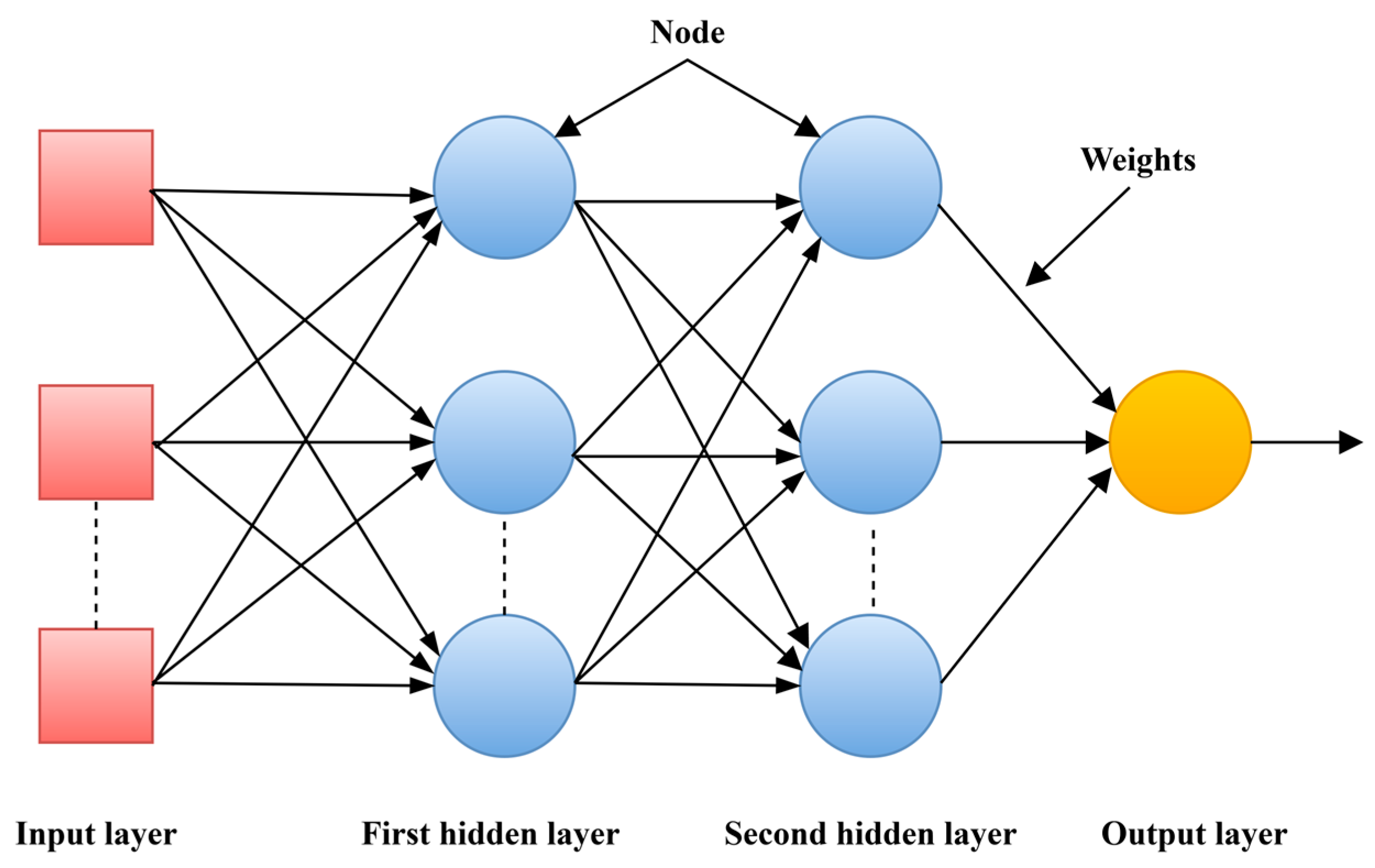
2.4.3. Multilayer Perceptron Classifier

In the multilayer perceptron classifier, neural networks have been utilized [28]. The network is structured as a feed-forward with many layers. Figure 2 shows the sort of network that contains one or more hidden layers of nodes in between both input and output layers. These nodes are linked together by a network that uses weights. Before controlling the layers that are being input and output, intermediary calculations are performed on the hidden layer.

3. Experimental Study

In this experimental investigation, the Machinery Fault Simulator, abbreviated as MFS, was utilized for acquiring the gear vibration signals. Figure 3 illustrates a schematic representation of the MFS. The experimental apparatus included a three-phase alternating current motor that served as the prime mover (3/4 horsepower, 2850 revolutions per minute). This motor was linked to the shaft using a flexible connection. On the other side of the shaft was a coupled belt and pulley agreement, which was then coupled with a straight-tooth bevel gearbox.

Table 1. Technical specifications of the single-stage bevel gearbox.

Description	Value
Module	2 mm
The angle of a pitch for gear	56°19′
The angle of a pitch for pinion	33°41′
No. of teeth (pinion)	18
Gear ratio	1.5:1
No. of teeth (gear)	27
Pressure angle	20°
Material (gear)	Forged steel
Material (pinion)	Forged steel

provides the bevel gearbox’s detailed technical specifications for this work. For this study, the level of crack faults made by the CNC Wire Electrical Discharge Machine (Wire EDM, Company name: Electronica India Limited, Pune (India), Model: ELPlus 15) is shown in Figure 4. In addition, the length of the crack was evaluated using an optical microscope. Figure 5 depicts the health of gears, whereas

Table 2. Details of the types of gear tooth cracks and their relative crack length in bevel gears.

S. No.	Types of Gear Tooth Crack	Crack Image	Crack Length (mm)
1.	Incipient crack tooth		0.25
2.	Slight crack tooth		0.50
3.	Moderate crack tooth		0.75
4.	Severe crack tooth		1.00

shows the types of gear tooth cracks and their relative length in straight bevel gears.

The studies were carried out with the motor operating at a speed range of 15–30 Hz. The motor’s speed was manually controlled using the controller. Additionally, a load of 0–4 Nm was applied to the gearbox’s output shaft using the mechanically controllable magnetic brake. A direct adhesive mounting method was employed for fastening a triaxial accelerometer to the upper surface of the housing of the bearing. This agreement was used to collect gear vibration data. The acceleration readings were recorded with a sample rate of 12.8 kHz in each of the three different directions (x, y, and z) simultaneously. Instead of showing all the directions of the vibration signal, only the z-direction is displayed in

Table 3. The z-direction of vibration signal for gears with different levels of crack faults.

The State of the Bevel Gear	Signal in the z-Direction (Vibration Signal)
Healthy gear
Incipient crack tooth
Slight crack tooth
Moderate crack tooth
Severe crack tooth

. From Table 3, it is shown that the time domain vibration signals vary in amplitude with the respective sample numbers. It was acquired for gears that have varying degrees of crack defects.

4. Results and Discussion

In this work, automated gear defect diagnostics using two different techniques, EWT and the proposed method, FBSE-EWT, also found the comparison performance. For the decomposition of signal input parameters such as global trend removal “none”, regularization “gaussian”, detection method “locmax”, and maximum number of bands “10” were used, respectively. Figure 6a,b shows the EWT-based decomposed sub-bands for all gear signals (healthy signal, incipient crack signal, slight crack signal, moderate crack signal, and severe crack signal) with the magnitude spectrum of their respective sub-bands. Figure 7 represents one example of scale–space-based determined boundaries in the FBSE-based magnitude spectrum. Further, it has been used to develop the FBSE-EWT-based filter bank shown in Figure 8. The spectrum analysis is improved by using the FBSE-EWT approach, as illustrated in Figure 9a,b for the same identical signals. Kurtosis, root mean square (RMS), variance, and Shannon entropy were some of the main characteristics that were extracted using the sub-bands. The Kruskal–Wallis test is conducted to see if there are substantive distinctions between the categories. A calculation of probability, denoted by p, was used to measure it.

Table 4. Obtained p-value for various features from EWT and FBSE-EWT approach.

Methods	EWT				FBSE-EWT (Proposed Method)
Bands	Kurtosis	RMS	Variance	Shannon Entropy	Kurtosis	RMS	Variance	Shannon Entropy
Sub-band 1	1.0591 × 10−9	7.6275 × 10−5	7.7517 × 10−5	4.7474 × 10−7	1.2526 × 10−6	0	0	0
Sub-band 2	0	0	0	0	1.3039 × 10−6	0	0	0
Sub-band 3	0.0001	0	0	0	0	1.0831 × 10−7	1.0839 × 10−7	3.4883 × 10−8
Sub-band 4	0.0021	0	0	0	1.3918 × 10−8	0	0	0
Sub-band 5	0.0001	0	0	0	0.008	0	0	0
Sub-band 6	0.0010	0	0	0	0.0111	0	0	0
Sub-band 7	0.0075	0	0	0	0.0020	0	0	0
Sub-band 8	0.7022	0	0	0	0.0029	9.0985 × 10−9	0	8.0157 × 10−9
Sub-band 9	0.4692	0	0	0	0.0034	1.8916 × 10−7	1.8847 × 10−7	1.4926 × 10−7
Sub-band 10	0	0	0	0	0	0	0	0

shows the EWT and FBSE-EWT p-values for 120 different pairs of gear crack signals. Also from Table 4, the statistical analysis indicated that it is necessary to omit the sub-band signal for those with p-values that are more than 0.05. The classifier obtains the significant statistical features that are extracted from the retentates. There are three different classifiers utilized in the method that has been presented, i.e., random forest, J48 decision tree classifiers, and multilayer perceptron function classifier. To train the classifiers, the 10-fold cross-validation method was applied to both the training data sets and the testing data sets. This was performed so that the classifiers could be properly evaluated.

The complete data set is randomly divided into two groups throughout the cross-validation process. The first group is called the training set and it contains 90 percent of the total data. The second group is called the testing set (10 percent). The procedures were carried out 10 times to conduct 10-fold cross-validation, which removes any potential sources of bias from the process of separating data into training and testing data sets.

Table 5. Performance comparison of classifiers between EWT and FBSE-EWT methods.

S. No.	Features	Performance of the Classifiers (%) Using EWT			Performance of the Classifiers (%) Using FBSE-EWT (Proposed Method)
		Random Forest	Multilayer Perceptron	J48	Random Forest	Multilayer Perceptron	J48
1	Kurtosis	57	43.5	40	77.5	55	42
2	RMS	62.5	51.5	52	67	61.5	51
3	Variance	59	46	43.5	68.5	48.5	43.5
4	Shannon entropy	59.5	59.5	44	67.5	46.5	44
5	Kurtosis and RMS	66.5	55	50	83.5	66	53
6	Kurtosis and variance	66	51.5	53	73	62.5	53.5
7	Kurtosis and Shannon entropy	68.5	50.5	49	84	73	55
8	RMS and variance	59	54	46	66.5	63	46
9	RMS and Shannon entropy	59	53	43	69.5	60	50
10	Variance and Shannon entropy	61	48	41	69.5	48	41
11	Kurtosis, RMS, and variance	65.5	54	44	72.5	68	46.5
12	Kurtosis, variance, and Shannon entropy	66	54.5	42	73	61.5	43
13	RMS, variance, and Shannon entropy	60	51.5	49	64.5	55	49
15	RMS, Shannon entropy, and kurtosis	66.5	53.5	39	82.5	72.5	39

shows the optimized classification results, with the objective of maximizing classification accuracy. According to Table 5, for EWT-based individual features and their combination features, including kurtosis, RMS, variance, and Shannon entropy, the random forest classifier showed the highest possible performance accuracy with 57%, 62.5%, 59%, 59.5%, 66.5%, 66%, 68.5%, 59%, 59%, 61%, 65.5%, 66%, 60%, and 66.5% accuracy, respectively. Additionally, the random forest classifier has demonstrated a high level of accuracy with 77.5%, 67%, 68.5%,67.5%, 83.5%, 73%, 84%, 66.5%, 69.5%, 69.5%, 72.5%, 73%, 64.5%, and 82.5% from Table 5 in FBES-EWT based on the same feature combination. According to Table 5, FBES-EWT achieved the highest classification accuracy, which was 84%, by employing a random forest classifier that incorporated the kurtosis and Shannon entropy characteristics.

The comparison of accuracy between our proposed method with gear signals and other existing methods in the literature is detailed in

Table 6. Comparison of proposed method with exiting methods.

Authors	Vibration Signal	Method	Feature	Classifier	Accuracy (%)
Saravanan et al. [15]	Bevel gearbox signals	CWT	Statistical features	ANN	97.5
Saravanan et al. [16]	Bevel gearbox signals	DWT	Statistical features	ANN	95
Proposed method	Bevel gearbox signals	FBSE-EWT	Kurtosis and Shannon entropy	Random forest	84

. Here, the authors are the first to apply the FBSE-EWT method to the mechanical system in gear fault deduction, which is the key novelty of this work. The maximum classification accuracy, i.e., 84%, has been achieved. On comparing the obtained accuracy of the proposed method with other existing methods, there is a marginal difference of 11%, which can be further improved by small training results. The results show that the proposed method has promising future uses in machine learning algorithms for building a knowledge base system that can aid in the early detection of defects, the implementation of condition-based maintenance to avoid catastrophic failure, and the reduction in operating costs.

5. Conclusions

Any malfunction in gear systems increases maintenance costs and downtime. Automated fault diagnosis of such systems could be a promising way to deal with such conditions. The EWT and FBSE-EWT methods have been used to decompose different levels of bevel gear crack fault signals. The obtained sub-bands are used to evaluate features. To improve the realization, statistically significant features with p < 0.05 are decided using the Kruskal–Wallis statistical test. These statistically significant features are fed to the classifiers. The maximum classification accuracy of 84% is obtained using the FBSE-EWT method with a random forest classifier for kurtosis and Shannon entropy features.

It is observed that FBSE-EWT is better than EWT for gear fault deduction. It is also observed that the classification accuracy for the random forest is better than that of multilayer perceptron and J48 classifiers. Comparative studies provide confirmatory evidence that the proposed approach, FBSE-EWT, is superior to EWT. Moreover, the present investigation and findings of the proposed methodology are quite helpful for the automatic identification of crack gear faults to diagnose the system with good accuracy.

References

- Sheng, S. Monitoring of Wind Turbine Gearbox Condition through Oil and Wear Debris Analysis: A Full-Scale Testing Perspective. Tribol. Trans. 2016, 59, 149–162. [Google Scholar] [CrossRef]
- Nowakowski, T.; Tomaszewski, F.; Komorski, P.; Szymański, G.M. Tram Gearbox Condition Monitoring Method Based on Trackside Acoustic Measurement. Measurement 2023, 207, 112358. [Google Scholar] [CrossRef]
- Bagavathiappan, S.; Lahiri, B.B.; Saravanan, T.; Philip, J.; Jayakumar, T. Infrared Thermography for Condition Monitoring—A Review. Infrared Phys. Technol. 2013, 60, 35–55. [Google Scholar] [CrossRef]
- Su, Y.; Meng, L.; Kong, X.; Xu, T.; Lan, X.; Li, Y. Small Sample Fault Diagnosis Method for Wind Turbine Gearbox Based on Optimized Generative Adversarial Networks. Eng. Fail. Anal. 2022, 140, 106573. [Google Scholar] [CrossRef]
- Jing, L.; Zhao, M.; Li, P.; Xu, X. A Convolutional Neural Network Based Feature Learning and Fault Diagnosis Method for the Condition Monitoring of Gearbox. Measurement 2017, 111, 1–10. [Google Scholar] [CrossRef]
- Lv, Y.; Zhao, W.; Zhao, Z.; Li, W.; Ng, K.K.H. Vibration Signal-Based Early Fault Prognosis: Status Quo and Applications. Adv. Eng. Inform. 2022, 52, 101609. [Google Scholar] [CrossRef]
- Mahgoun, H.; Chaari, F.; Felkaoui, A. Detection of Gear Faults in Variable Rotating Speed Using Variational Mode Decomposition (VMD). Mech. Ind. 2016, 17, 207. [Google Scholar] [CrossRef]
- Wang, W. Early Detection of Gear Tooth Cracking Using the Resonance Demodulation Technique. Mech. Syst. Signal Process. 2001, 15, 887–903. [Google Scholar] [CrossRef]
- Wang, D. K-Nearest Neighbors Based Methods for Identification of Different Gear Crack Levels under Different Motor Speeds and Loads: Revisited. Mech. Syst. Signal Process. 2016, 70–71, 201–208. [Google Scholar] [CrossRef]
- Yang, X.; Wang, L.; Ding, K.; Ding, X. Vibration AM-FM Sidebands Mechanism of Planetary Gearbox with Tooth Root Cracked Planet Gear. Eng. Fail. Anal. 2022, 137, 106353. [Google Scholar] [CrossRef]
- Aherwar, A. An Investigation on Gearbox Fault Detection Using Vibration Analysis Techniques: A Review. Aust. J. Mech. Eng. 2012, 10, 169–183. [Google Scholar] [CrossRef]
- Staszewski, W.J.; Tomlinson, G.R. Local Tooth Fault Detection in Gearboxes Using a Moving Window Procedure. Mech. Syst. Signal Process. 1997, 11, 331–350. [Google Scholar] [CrossRef]
- Cheng, G.; Cheng, Y.L.; Shen, L.H.; Qiu, J.B.; Zhang, S. Gear Fault Identification Based on Hilbert-Huang Transform and SOM Neural Network. Measurement 2013, 46, 1137–1146. [Google Scholar] [CrossRef]
- Upadhyay, N.; Kankar, P.K. Diagnosis of Bearing Defects Using Tunable Q-Wavelet Transform. J. Mech. Sci. Technol. 2018, 32, 549–558. [Google Scholar] [CrossRef]
- Saravanan, N.; Siddabattuni, V.N.S.K.; Ramachandran, K.I. Fault Diagnosis of Spur Bevel Gear Box Using Artificial Neural Network (ANN), and Proximal Support Vector Machine (PSVM). Appl. Soft Comput. J. 2010, 10, 344–360. [Google Scholar] [CrossRef]
- Saravanan, N.; Ramachandran, K.I. Incipient Gear Box Fault Diagnosis Using Discrete Wavelet Transform (DWT) for Feature Extraction and Classification Using Artificial Neural Network (ANN). Expert Syst. Appl. 2010, 37, 4168–4181. [Google Scholar] [CrossRef]
- Li, C.; Sanchez, R.V.; Zurita, G.; Cerrada, M.; Cabrera, D.; Vásquez, R.E. Gearbox Fault Diagnosis Based on Deep Random Forest Fusion of Acoustic and Vibratory Signals. Mech. Syst. Signal Process. 2016, 76–77, 283–293. [Google Scholar] [CrossRef]
- Lobato, T.H.G.; da Silva, R.R.; da Costa, E.S.; Mesquita, A.L.A. An Integrated Approach to Rotating Machinery Fault Diagnosis Using, EEMD, SVM, and Augmented Data. J. Vib. Eng. Technol. 2020, 8, 403–408. [Google Scholar] [CrossRef]
- Han, D.; Zhao, N.; Shi, P. Gear Fault Feature Extraction and Diagnosis Method under Different Load Excitation Based on EMD, PSO-SVM and Fractal Box Dimension. J. Mech. Sci. Technol. 2019, 33, 487–494. [Google Scholar] [CrossRef]
- Kim, B.; Lee, J. Fault Diagnosis and Noise Robustness Comparison of Rotating Machinery Using CWT and CNN. Adv. Sci. Technol. Eng. Syst. J. 2021, 6, 1279–1285. [Google Scholar] [CrossRef]
- Mallat, S. A Theory for Multi-Resolution Signal Decomposition Wavelet Representation. IEEE Trans. Pattern Anal. Mach. Intell. 1989, 11, 674–693. [Google Scholar] [CrossRef]
- Syed, S.H.; Muralidharan, V. Feature Extraction Using Discrete Wavelet Transform for Fault Classification of Planetary Gearbox—A Comparative Study. Appl. Acoust. 2022, 188, 108572. [Google Scholar] [CrossRef]
- Ramteke, D.S.; Parey, A.; Pachori, R.B. Automated Gear Fault Detection of Micron Level Wear in Bevel Gears Using Variational Mode Decomposition. J. Mech. Sci. Technol. 2019, 33, 5769–5777. [Google Scholar] [CrossRef]
- Gilles, J. Empirical Wavelet Transform. IEEE Trans. Signal Process. 2013, 61, 3999–4010. [Google Scholar] [CrossRef]
- Bhattacharyya, A.; Singh, L.; Pachori, R.B. Fourier-Bessel Series Expansion Based Empirical Wavelet Transform for Analysis of Non-Stationary Signals. Digit. Signal Process. 2018, 78, 185–196. [Google Scholar] [CrossRef]
- Kedadouche, M.; Thomas, M.; Tahan, A. A Comparative Study between Empirical Wavelet Transforms and Empirical Mode Decomposition Methods: Application to Bearing Defect Diagnosis. Mech. Syst. Signal Process. 2016, 81, 88–107. [Google Scholar] [CrossRef]
- Kumar, A.; Parey, A.; Kankar, P.K. Supervised Machine Learning Based Approach for Early Fault Detection in Polymer Gears Using Vibration Signals. Mapan-J. Metrol. Soc. India 2023, 38, 383–394. [Google Scholar] [CrossRef]
- Saravanan, N.; Cholairajan, S.; Ramachandran, K.I. Vibration-Based Fault Diagnosis of Spur Bevel Gear Box Using Fuzzy Technique. Expert Syst. Appl. 2009, 36, 3119–3135. [Google Scholar] [CrossRef]
- Muralidharan, A.; Sugumaran, V.; Soman, K.P.; Amarnath, M. Fault Diagnosis of Helical Gear Box Using Variational Mode Decomposition and Random Forest Algorithm. Struct. Durab. Health Monit. 2014, 10, 55. [Google Scholar]
- Zhang, Y.; Yu, K.; Lei, Z.; Ge, J.; Xu, Y.; Li, Z.; Ren, Z.; Feng, K. Integrated Intelligent Fault Diagnosis Approach of Offshore Wind Turbine Bearing Based on Information Stream Fusion and Semi-Supervised Learning. Expert Syst. Appl. 2023, 232, 120854. [Google Scholar] [CrossRef]
- Zhang, Y.; Ji, J.C.; Ren, Z.; Ni, Q.; Gu, F.; Feng, K.; Yu, K.; Ge, J.; Lei, Z.; Liu, Z. Digital Twin-Driven Partial Domain Adaptation Network for Intelligent Fault Diagnosis of Rolling Bearing. Reliab. Eng. Syst. Saf. 2023, 234, 109186. [Google Scholar] [CrossRef]
- Chen, Z.Q.; Li, C.; Sanchez, R.V. Gearbox Fault Identification and Classification with Convolutional Neural Networks. Shock Vib. 2015, 2015, 390134. [Google Scholar] [CrossRef]
- Kateris, D.; Moshou, D.; Pantazi, X.E.; Gravalos, I.; Sawalhi, N.; Loutridis, S. A Machine Learning Approach for the Condition Monitoring of Rotating Machinery. J. Mech. Sci. Technol. 2014, 28, 61–71. [Google Scholar] [CrossRef]
- Schroeder, J. Signal Processing via Fourier-Bessel Series Expansion. Digit. Signal Process. 1993, 3, 112–124. [Google Scholar] [CrossRef]
- Sharma, V.; Parey, A. A Review of Gear Fault Diagnosis Using Various Condition Indicators. Procedia Eng. 2016, 144, 253–263. [Google Scholar] [CrossRef]
- Kruskal, W.H.; Wallis, W.A. Use of Ranks in One-Criterion Variance Analysis. J. Am. Stat. Assoc. 1952, 47, 583. [Google Scholar] [CrossRef]
- Breiman, L. Random Forests. Mach. Learn. 2001, 45, 5–32. [Google Scholar] [CrossRef]
Figure 1.
A block diagram showing the suggested approach.
Figure 2.
Graphical description of a multilayer perceptron.
Figure 3.
Schematic presentation of the experimental setup.
Figure 4.
Crack faults created by the CNC wire (EDM) machine.
Figure 5.
Health of the straight-tooth bevel gears: (a) healthy gear; (b) gear with a 0.25 mm crack length; (c) gear with a 0.50 mm crack length; (d) gear with a 0.75 mm crack length; (e) gear with a 1.00 mm crack length.
Figure 6.
(a) Applied EWT decomposition and find sub-bands; (b) representation of the magnitude spectrum of their respective sub-bands.
Figure 7.
FBSE magnitude-spectrum-based determined boundaries.
Figure 8.
Developed FBSE-EWT-based filter bank.
Figure 9.
(a) Applied FBSE-EWT decomposition and found sub-bands; (b) representation of the magnitude spectrum of their respective sub-bands.