Exact Formulation for the Curvature of Gothic Arch Ball Screw Profiles and New Approximated Solution Based on Simplified Groove Geometry

Abstract

The correct evaluation of the curvatures of ball screw grooves allows the accurate design of the constructive parameters of this mechanism and enhancing its performance. The formulation commonly used in the literature, however, refers to ball bearing geometry, ignoring the shape of the section’s profile and the helix angle. In this paper, the exact formulae for calculating the principal curvature radii of the screw shaft and the nut grooves are analytically derived and presented. These equations, obtained through a rigorous differential geometry approach, consider the helix angle and a gothic arch profile. An approximated formulation is proposed simplifying the exact solution under the assumption of a circular groove profile. These new simple formulae accurately reproduce the exact curvature radii values with a mean relative error of approximatively 0.51% and 0.40%, respectively, for the screw shaft and nut grooves, against the value of more than 50% obtained by using the literature formulae for common off-the-shelf ball screws, especially those with high helix angles. Furthermore, they allow a computational time saving of 98%, making them suitable for being incorporated in high-fidelity dynamic models of ball. Finally, two MATLAB functions are provided to easily evaluate the complex curvature exact solution.

1. Introduction

Ball screws are mechanical components used to convert the rotational motion into a linear displacement and vice versa. The mechanism is mainly composed of a threaded shaft and one or two nuts like in traditional sliding screws. However, in contrast to the latter, ball screws present a set of spheres interposed between the grooves of the screw and the nuts, which act as a rolling interface allowing the mechanical efficiency to move from a typical value of 0.3–0.5 to values usually higher than 0.9. This result can be achieved because the slipping between the grooves of classic lead screws is replaced by the rolling motion of the spheres, which generates a remarkably lower friction.

These mechanisms are used in many different sectors, such as manufacturing, robotics and aerospace, thanks to their very high efficiency, stiffness and positioning precision [1,2]. Nevertheless, full awareness of what happens within the system has not yet been achieved and, due to its complexity, experimental analyses of the internal mechanical behaviour have been performed only in very simplified conditions [3,4].

Despite the ball screw mechanism having been used since the first years of the last century, its inherent complexity has led the first theoretical analyses to be carried out only after several decades of usage [5]. More recently, several researchers have focused on the study of this component, analysing it from many different points of view. A major contribution to the theoretical analysis of the internal kinematics was provided by Lin et al. [6,7] and Wei et al. [8] who studied the mechanical efficiency of single nut ball screws under quasi-static conditions. Wei et al. [9] analysed the link between the mechanical efficiency and the preload. The kinematics of high speed ball screws were investigated by Wei et al. [10] and Xu et al. [11], who identified the geometrical parameters for reducing the slipping between spheres and grooves. Indeed, the greater the internal slippage, the higher the overall friction torque. The latter and its correlation with the preload was studied by Verl and Frey [12], Zhou et al. [13] and Bertolino et al. [14].

Because of the low friction torque, the high efficiency, the elevated stiffness and the possibility to compensate the backlash with preload, ball screws are employed in those systems which require a high positioning accuracy: therefore, various investigations have been carried out to understand the influence of preload, temperature and control strategies on this aspect [15,16,17,18].

The expected duration of a ball screw is related to many external factors, such as environmental and operative conditions or control strategies [19], but also to the correct design of the mechanism itself. In fact, an excessive load on the spheres can lead to accelerated wear and flaws in the grooves, with a consequent increase of the vibration level, deterioration of the mechanism’s performance and, eventually, premature failure or jamming of the transmission. For this reason, several researchers have focused on the study of the static load distribution among the spheres [20,21,22] and how it is modified by the interaction of the different deformation modes [23]. Oyanguren et al. [24] investigated the influence of the thermal deformation on the load distribution caused by friction heating in dynamic conditions.

A new frontier in the research on this mechanism is the possibility to anticipate certain kinds of performance reduction, or even failures, monitoring some health features coming from the mechanism itself or from a combination of signals from the other ball screw drive components [25,26,27]. Hence, studies have been performed to investigate preload degradation [27,28], wear [29,30,31,32] and the recirculating circuit design [33,34]. In this framework, the authors developed a full dynamic model of an entire double nut ball screw taking into account the recirculation channel [35] and the presence of lubricant [36], with 3D internal contact description [37], in order to investigate the interaction of different defects and their time evolution, as well as the variation of internal contact conditions and of internal kinematic and dynamic quantities during the mechanism’s operation, removing the quasi static assumption of previous studies. The model provides the basis for detailed prognostic investigations on ball screws [38], which are one of the most critical components of ball screw drives. In order to validate this model, an innovative test bench was designed [39,40].

One common aspect is common to all these cited studies carried out on ball screws, and that is the radii calculation of the grooves’ curvature. Indeed, force is transmitted between the screw shaft and the nuts through the spheres, which results in compression, and hence, a contact pressure arises in each contact point whose value depends on the surface features of the two mating geometries. Hitherto, the curvature of the groove of the screw shaft and the nut has been calculated according to the formula suggested in the ISO3408 international standard [41] and in various manufacturers’ catalogues. This formula comes from bearings theory and does not take into account either the helical shape of the grooves or the gothic arch profile of its section. The error committed using the bearing formula to calculate the curvature of the groove mainly increases with the helix angle, while the two values obviously converge when the helix angle tends towards zero.

This paper presents the exact formulation for the curvature of the grooves of screw and nuts, in order to consider all these geometrical parameters: two MATLAB functions to calculate the correct values are provided as companion files to this article. Since the exact formulation is a fairly long and complex expression, not suitable for fast hand calculations or to be implemented in simulation environments, the authors developed two approximated formulae to obtain, with a reasonable small relative error, the curvature values of the screw and nut grooves.

The possibility of a precise fast formula for calculating the curvatures of the grooves is paramount for those applications in which the accuracy of results is important, such as the development of high-fidelity models for prognostic activities or for real-time applications. In fact, such models should run in extensive simulation campaigns and the need for accuracy must meet the necessity of reduced computation time. The proposed approximated formulation sensibly reduces the approximation errors without adding any substantial computational effort.

2. Materials and Methods

Since the ball screw theory directly derives from the well-developed knowledge on ball bearings, many concepts remain unvaried. Among them, the curvatures of ball screw grooves have commonly been calculated with the simple formulae indicated in the ISO3408-5:2006 standard [41] and in manufacturers’ catalogues. However, this method disregards the effect of the shape of the groove profile (circular or gothic arch) and, in particular, of the helix angle. This section describes the derivation of the exact formulation presented in this paper for the evaluation of the principal curvatures of both the screw and nut grooves.

2.1. Groove Geometry of Ball Screws

Considering a right-hand threaded ball screw, the grooves of the screw and the nut can be described starting from the ideal helix with radius $r_m$ (the pitch circle radius) and a helix angle equal to ${\alpha }_e$, shown in Figure 1. This helix represents the locus of all the ideal positions that a generic sphere can assume. In order to mathematically describe the groove geometry, two coordinate systems (CS) must be introduced:

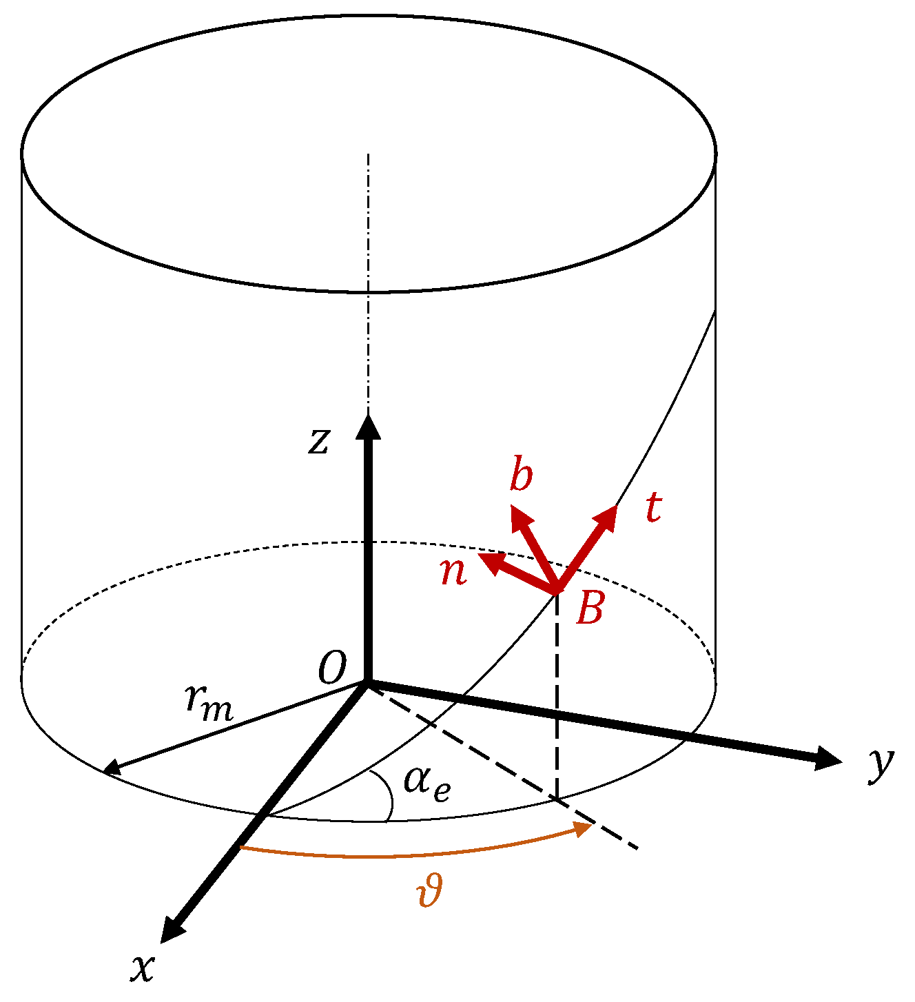
• $Oxyz$ is the screw shaft CS, with the z axis aligned along the screw shaft axis;
• $Btnb$ is the Frenet–Serret CS, whose centre B is located on the helix, with the t axis tangent to it, the n axis directed perpendicularly toward the screw shaft axis z and the b axis perpendicular to t and n axes to create a right-handed CS. The origin B of this CS identifies the ideal position of the centre of the sphere, and its location, with regards to the screw shaft’s CS $Oxyz$, is defined by the azimuth angle $\vartheta$.

It is assumed that the helix starts on the x axis, in the point with coordinates $(r_m,0,0)$ expressed in the $Oxyz$ CS (Figure 1). The rotation matrices linking these CSs can be easily constructed referring to Figure 1 and can be found in [6]. In particular, ${\mathrm{T}}_{BO}$ is the rotation matrix to transform a vector expressed in the $Oxyz$ CS in the Frenet–Serret CS.

The location of the centre B of the Frenet–Serret reference frame with respect to the centre O of the screw CS (subscript B/O) expressed in the screw CS (superscript O) can be written as follows:

$${\mathbf{R}}_{B/O}^O=r_m{[cos\left(\vartheta \right)sin\left(\vartheta \right)\vartheta tan\left({\alpha }_e\right)]}^T$$

(1)

Observing a section normal to the thread, i.e. on a plane containing the n and b axes, the profile of the grooves can be identified. To remain as general as possible, this paper considers a gothic arch groove profile. Each of the two raceways of the screw shaft and the nut is composed by two half grooves, whose profiles are two circular segments with radius $r_s$. Offsetting the centre C of this circle with respect to B, as shown in Figure 2a, by the centre radius offset H and the ogival offset L, respectively along the n and b axes, the gothic arch profile is obtained. The formulation for the circular profile groove can be easily obtained by imposing $L=0$.

In order to create a sufficiently localised contact point and to reduce the slippage within the contact area, the following condition on the ratio between the groove radius $r_s$ and the ball diameter $D_b$, called the conformity factor $f_s$, must hold:

$$f_s=\frac{r_s}{D_b}>0.5$$

(2)

Although ideally the ball and the grooves would perfectly mate tangentially, as shown in Figure 2a, in real components a little amount of internal play is always present because of the manufacturing tolerances and the mounting requirements (except for the case in which the preload is obtained with oversized balls [15]). Therefore, the contact angle $\phi$ would move slightly from the theoretical one ${\phi }_0$ decided during the design phase, and it varies during ball screw life because of different actual dimensions, loading conditions and the wear of balls and grooves.

Knowing the ball radius, the desired theoretical contact angle and the conformity factor, the offsets H and L can be determined with the following equations:

$$L=(r_s-r_b)sin\left({\phi }_0\right)$$

(3)

$${\phi }_0=arctan\left(\frac{L}{H}\right)$$

(4)

From now on, only one of the two half grooves of the screw shaft will be analysed (the left one of Figure 2a) because of the symmetry of the groove’s profile. Once the location of the centre C is defined with respect to B, each point of the half groove profile can be identified by varying the contact angle $\phi$. Therefore, the position of a generic point P on the groove’s profile with respect to B can be expressed with the following coordinates in the Frenet–Serret CS (superscript B) as:

$${\mathbf{R}}_{P/B,screw}^B={[0-H+r_{s}cos\left(\phi \right)L-r_{s}sin\left(\phi \right)]}^T$$

(5)

Therefore, the entire half groove geometry can be expressed in the $Oxyz$ CS as:

$${\mathbf{R}}_{P/O,screw}^O={\mathrm{T}}_{BO}^T{\mathbf{R}}_{P/B,screw}^B+{\mathbf{R}}_{B/O}^O$$

(6)

which represents a parametric description of the screw’s half groove surface as a function of the azimuth angle $\vartheta$ and the contact angle $\phi$:

$${\mathbf{R}}_{P/O,screw}^O=\left[\begin{array}{c}-[r_{s}sin\left({\alpha }_e\right)sin\left(\phi \right)-Lsin\left({\alpha }_e\right)]sin\left(\vartheta \right)+[H+r_m-r_{s}cos\left(\phi \right)]cos\left(\vartheta \right)\\ [r_{s}sin\left({\alpha }_e\right)sin\left(\phi \right)-Lsin\left({\alpha }_e\right)]cos\left(\vartheta \right)+[H+r_m-r_{s}cos\left(\phi \right)]sin\left(\vartheta \right)\\ r_m\vartheta tan\left({\alpha }_e\right)+Lcos\left({\alpha }_e\right)-r_{s}cos\left({\alpha }_e\right)sin\left(\phi \right)\end{array}\right]$$

(7)

The parametrization of one half groove of the nut raceway, shown in Figure 2b, can be obtained with the same approach. Equation (6) becomes:

$${\mathbf{R}}_{P/O,nut}^O={\mathrm{T}}_{BO}^T{\mathbf{R}}_{P/B,nut}^B+{\mathbf{R}}_{B/O}^O$$

(8)

where

$${\mathbf{R}}_{P/B,nut}^B={[0H-r_{s}cos\left(\phi \right)L-r_{s}sin\left(\phi \right)]}^T$$

(9)

Finally, the parametric description of the nut half groove surface as a function of the azimuth angle $\vartheta$ and the contact angle $\phi$ can be obtained:

$${\mathbf{R}}_{P/O,nut}^O=\left[\begin{array}{c}-[r_{s}sin\left({\alpha }_e\right)sin\left(\phi \right)-Lsin\left({\alpha }_e\right)]sin\left(\vartheta \right)+[-H+r_m+r_{s}cos\left(\phi \right)]cos\left(\vartheta \right)\\ [r_{s}sin\left({\alpha }_e\right)sin\left(\phi \right)-Lsin\left({\alpha }_e\right)]cos\left(\vartheta \right)+[-H+r_m+r_{s}cos\left(\phi \right)]sin\left(\vartheta \right)\\ r_m\vartheta tan\left({\alpha }_e\right)+Lcos\left({\alpha }_e\right)-r_{s}cos\left({\alpha }_e\right)sin\left(\phi \right)\end{array}\right]$$

(10)

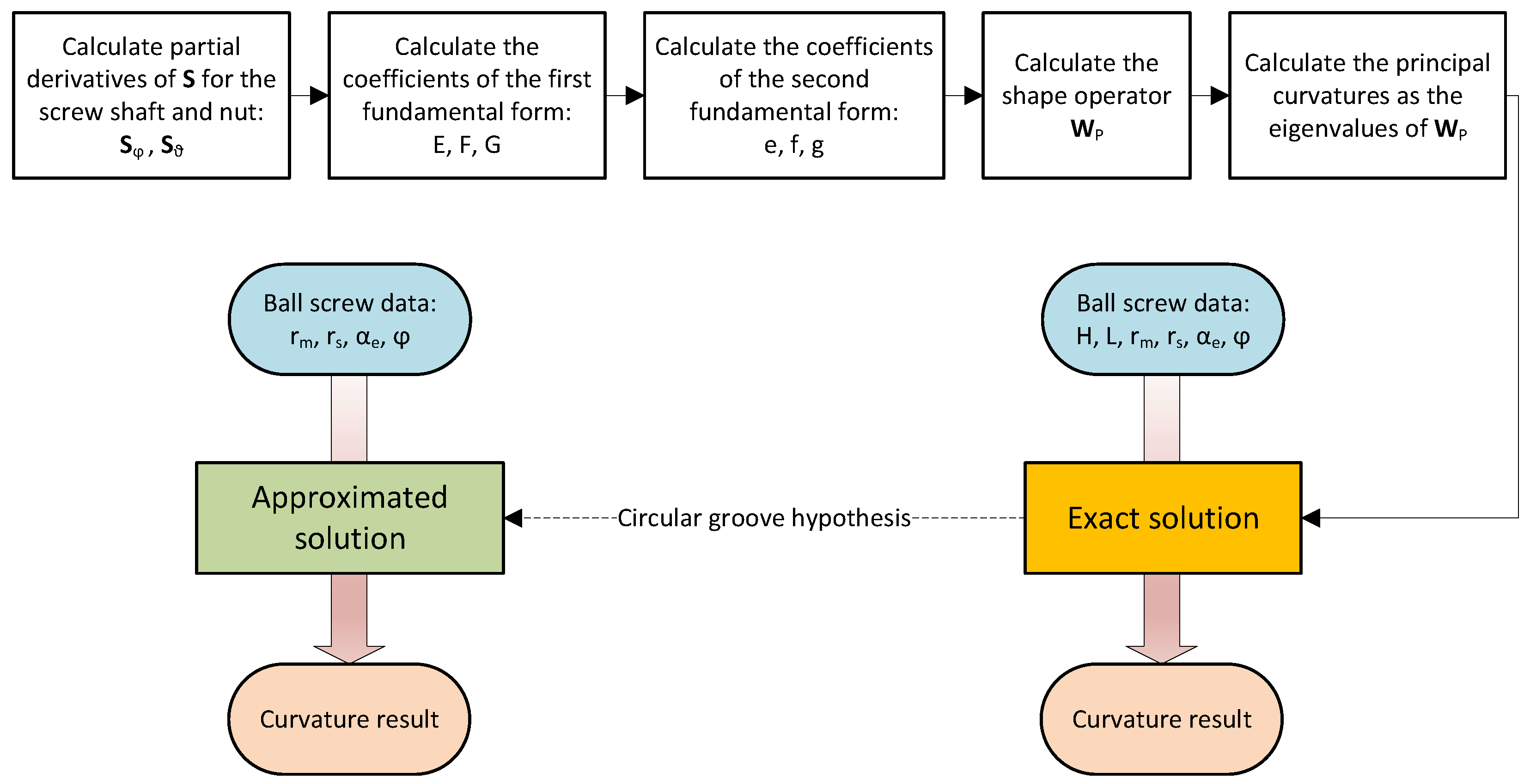
2.2. Exact Curvature Calculation

Equation (7) (or Equation (10) for the nut) represents a smooth regular parametrized surface in $\mathrm{I}{\mathrm{R}}^3$. Renaming this surface S, it is defined over the domain $\mathsf{\Omega }$, subspace of $\mathrm{I}{\mathrm{R}}^2$:

$$\mathbf{S}:\mathsf{\Omega }\to \mathrm{I}{\mathrm{R}}^3,(\vartheta ,\phi )\to \left[\begin{array}{c}{S}_1(\vartheta ,\phi )\\ S_2(\vartheta ,\phi )\\ S_3(\vartheta ,\phi )\end{array}\right]$$

(11)

where the components of $\mathbf{S}$ in the Cartesian space $S_1(\vartheta ,\phi )$, $S_2(\vartheta ,\phi )$ and $S_3(\vartheta ,\phi )$ are real functions of the parameters $(\vartheta ,\phi )\in \mathsf{\Omega }$.

Each point of $\mathbf{S}$ can thus be identified by choosing the values of these two parameters. Let $({\vartheta }_0,{\phi }_0)$ represent the point P on which the two principal curvatures of the groove must be calculated. For ball screw grooves, one of the two principal curvatures is simply $-1/r_s$, obtained on the section normal to the helix in P, and the curvature centre is simply point C. Instead, following the Meusnier theorem [42], the other principal curvature can be defined as the normal curvature of the curve $\gamma$ on $\mathbf{S}$, obtained intersecting the latter with a plane $\mathsf{\Pi }$, as shown in Figure 3. This curve $\gamma$ entirely lies on $\mathsf{\Pi }$, which is defined as the plane containing the t axis, tangent to $\gamma$ in P by definition, and containing the points P and C, hence also containing the vector normal to the surface in P.

The unit vector of the normal-to-the-surface $\mathbf{S}$ in P can be easily obtained as:

$$\mathbf{N}({\vartheta }_0,{\phi }_0)=\frac{{\mathbf{S}}_{\vartheta }({\vartheta }_0,{\phi }_0)\times {\mathbf{S}}_{\phi }({\vartheta }_0,{\phi }_0)}{∥{\mathbf{S}}_{\vartheta }({\vartheta }_0,{\phi }_0)\times {\mathbf{S}}_{\phi }({\vartheta }_0,{\phi }_0)∥}$$

(12)

where ${\mathbf{S}}_{\phi }=\frac{\partial \mathbf{S}}{\partial \phi }$ and ${\mathbf{S}}_{\vartheta }=\frac{\partial \mathbf{S}}{\partial \vartheta }$ are the two partial derivatives of $\mathbf{S}$ with respect to the free variables: they form a basis of the tangent space in $({\vartheta }_0,{\phi }_0)$. For the screw shaft groove, deriving Equation (7), they assume the following expressions:

$${\mathbf{S}}_{\phi ,screw}=r_s\left[\begin{array}{c}cos\left(\vartheta \right)sin\left(\phi \right)-cos\left(\phi \right)sin\left({\alpha }_e\right)sin\left(\vartheta \right)\\ sin\left(\phi \right)sin\left(\vartheta \right)+cos\left(\phi \right)sin\left({\alpha }_e\right)cos\left(\vartheta \right)\\ -cos\left({\alpha }_e\right)cos\left(\phi \right)\end{array}\right]$$

(13)

$${\mathbf{S}}_{\vartheta ,screw}=\left[\begin{array}{c}\left[Lsin\left({\alpha }_e\right)-r_{s}sin\left({\alpha }_e\right)sin\left(\phi \right)\right]cos\left(\vartheta \right)+\left[r_{s}cos\left(\phi \right)-H-r_m\right]sin\left(\vartheta \right)\\ \left[H+r_m-r_{s}cos\left(\phi \right)\right]cos\left(\vartheta \right)+\left[Lsin\left({\alpha }_e\right)-r_{s}sin\left({\alpha }_e\right)sin\left(\phi \right)\right]sin\left(\vartheta \right)\\ r_{m}tan\left({\alpha }_e\right)\end{array}\right]$$

(14)

while for the nut they can be calculated deriving Equation (10), obtaining:

$${\mathbf{S}}_{\phi ,nut}=r_s\left[\begin{array}{c}-cos\left(\vartheta \right)sin\left(\phi \right)-cos\left(\phi \right)sin\left({\alpha }_e\right)sin\left(\vartheta \right)\\ cos\left(\phi \right)sin\left({\alpha }_e\right)cos\left(\vartheta \right)-sin\left(\phi \right)sin\left(\vartheta \right)+\\ -cos\left({\alpha }_e\right)cos\left(\phi \right)\end{array}\right]$$

(15)

$${\mathbf{S}}_{\vartheta ,nut}=\left[\begin{array}{c}\left[Lsin\left({\alpha }_e\right)-r_{s}sin\left({\alpha }_e\right)sin\left(\phi \right)\right]cos\left(\vartheta \right)+\left[H-r_{s}cos\left(\phi \right)-r_m\right]sin\left(\vartheta \right)\\ \left[r_m-H+r_{s}cos\left(\phi \right)\right]cos\left(\vartheta \right)+\left[Lsin\left({\alpha }_e\right)-r_{s}sin\left({\alpha }_e\right)sin\left(\phi \right)\right]sin\left(\vartheta \right)\\ r_{m}tan\left({\alpha }_e\right)\end{array}\right]$$

(16)

In order to calculate the first principal curvature of the groove, a semi-analytical approach could be used, in which the parametric expression of the groove has been equated to the parametric expression of the plane $\mathsf{\Pi }$, obtaining the expression of $\gamma$. However, as it was composed of a set of implicit equations, and an analytical closed form for the curvature was not found, a numeric approach was followed to solve the implicit system.

A more elegant way to obtain such curvature is presented in this paper and it consists in defining the Weingarten map ${\mathbf{W}}_P$ (called also shape operator) [43] of the surface $\mathbf{S}$ in P:

$${\mathbf{W}}_P={\mathbf{I}}^{-1}\mathbf{II}={\left[\begin{array}{cc}E& F\\ F& G\end{array}\right]}^{-1}\left[\begin{array}{cc}e& f\\ f& g\end{array}\right]=\frac{1}{EG-F^2}\left[\begin{array}{cc}Ge-Ff& Gf-Fg\\ Ef-Fe& Eg-Ff\end{array}\right]$$

(17)

where E, F, G and e, f, g are the respective coefficients of the first and second fundamental forms $\mathbf{I}$ and $\mathbf{II}$ of the surface $\mathbf{S}$ [44]:

$$E={\mathbf{S}}_{\phi }·{\mathbf{S}}_{\phi }$$

(18)

$$F={\mathbf{S}}_{\phi }·{\mathbf{S}}_{\vartheta }$$

(19)

$$G={\mathbf{S}}_{\vartheta }·{\mathbf{S}}_{\vartheta }$$

(20)

$$e={\mathbf{S}}_{\phi \phi }·\mathbf{N}=\frac{{\mathbf{S}}_{\phi }\times {\mathbf{S}}_{\vartheta }·{\mathbf{S}}_{\phi \phi }}{\sqrt{EG-F^2}}$$

(21)

$$f={\mathbf{S}}_{\phi \vartheta }·\mathbf{N}=\frac{{\mathbf{S}}_{\phi }\times {\mathbf{S}}_{\vartheta }·{\mathbf{S}}_{\phi \vartheta }}{\sqrt{EG-F^2}}$$

(22)

$$g={\mathbf{S}}_{\vartheta \vartheta }·\mathbf{N}=\frac{{\mathbf{S}}_{\phi }\times {\mathbf{S}}_{\vartheta }·{\mathbf{S}}_{\vartheta \vartheta }}{\sqrt{EG-F^2}}$$

(23)

with ${\mathbf{S}}_{\phi \phi }=\frac{{\partial }^2\mathbf{S}}{\partial {\phi }^2}$, ${\mathbf{S}}_{\vartheta \vartheta }=\frac{{\partial }^2\mathbf{S}}{\partial {\vartheta }^2}$ and ${\mathbf{S}}_{\phi \vartheta }=\frac{\partial {\mathbf{S}}_{\vartheta }}{\partial \phi }$ the second derivatives of the surface parametrization with respect to the free parameters.

Finally, the principal curvatures ${\kappa }_1$ and ${\kappa }_2$ of $\mathbf{S}$ are the eigenvalues of the shape operator defined in Equation (17), i.e., the roots of its characteristic polynomial:

$$\det \left(\mathbf{II}-\mathit{\kappa }\mathbf{I}\right)=\left(EG-F^2\right){\kappa }^2-\left(eG+Eg-2fF\right)\kappa +eg-f^2=0$$

(24)

The expressions resulting from the solution of Equation (24) represent a closed-form exact analytical solution for the principal curvatures of ball screw grooves. However, the expressions for both the screw shaft and nut grooves are fairly complex and too long to be included in the main text: for this reason they are reported in Appendix B and two MATLAB functions are made available as complementary material to this article for calculating the exact values of the principal curvatures of the grooves of the screw shaft and the nut. The inputs of both functions are H, L, ${\alpha }_e$, $\phi$, $r_m$ and $r_s$, while the outputs are the principal curvatures ${\kappa }_1$ and ${\kappa }_2$ from the solution of Equation (24). The triplet of parameters H, L and $r_s$ can be linked to the other parameters $r_b$, $f_s$ and ${\phi }_0$ through Equations (2)–(4). It is worth highlighting that the curvatures do not depend on the azimuth angle, since its effect is only to move the considered point P along the helix: hence, while the surface requires two free parameters to be described, the curvature only depends on the contact angle. Therefore, the equations contained in the provided functions have been simplified imposing $\vartheta =0$. Furthermore, the second principal curvature, on the plane $n-b$ normal to the thread in P, does not even depend on $\phi$, as the half groove is a circular segment: it is then completely defined by the design parameter $r_s$.

2.3. Approximated Formulation Assuming a Circular Groove Profile

While the two functions, available as supplemental material to this paper, represent the correct analytical expression of the curvatures of the grooves of the screw shaft and nut obtained from the solution of Equation (24), their formulations are quite complex and long, and a computer is generally required for their evaluation. For this reason, simplified short equations for both the screw shaft and nut grooves would be useful in real practice in order to easily and accurately describe the dependence of the first principal curvature radius on the helix angle.

A reasonable approximation can be made assuming a ball screw with a circular groove profile. If this hypothesis holds, the parameters L and H can be set to zero and the curvature expression from the solution of Equation (24) is simplified considerably. Therefore, the exact formulation (Equation (A1)) reduces to the following expression for the screw shaft:

$${\kappa }_{1s,circ}=\frac{cos\left(\phi \right){cos}^2\left({\alpha }_e\right)}{r_m-r_{s}cos\left(\phi \right){cos}^2\left({\alpha }_e\right)}$$

(25)

while for the nut groove it becomes:

$${\kappa }_{1n,circ}=-\frac{cos\left(\phi \right){cos}^2\left({\alpha }_e\right)}{r_m+r_{s}cos\left(\phi \right){cos}^2\left({\alpha }_e\right)}$$

(26)

In reality, the parameters L and H are not always equal to zero. Therefore, in same cases, it is still necessary to use Equation (24) to obtain the principal curvatures ${\kappa }_1$ and ${\kappa }_2$.

The outcomes of the two proposed approximated formulations for both the screw shaft and nut grooves will be discussed in the following section and the results will be compared with those of the exact solution and the common literature formulae.

Figure 4 graphically explains the aforementioned procedure followed to obtain both the exact and approximated formulations. Specifically, it shows in the upper part the analytical passages needed to formulate the exact solution, discussed in Section 2.2. Then, in the lower part, the simplifying approach to finding the approximated solution is represented. Once both formulations are present, given the input data, one of them can be chosen to obtain the desired result.

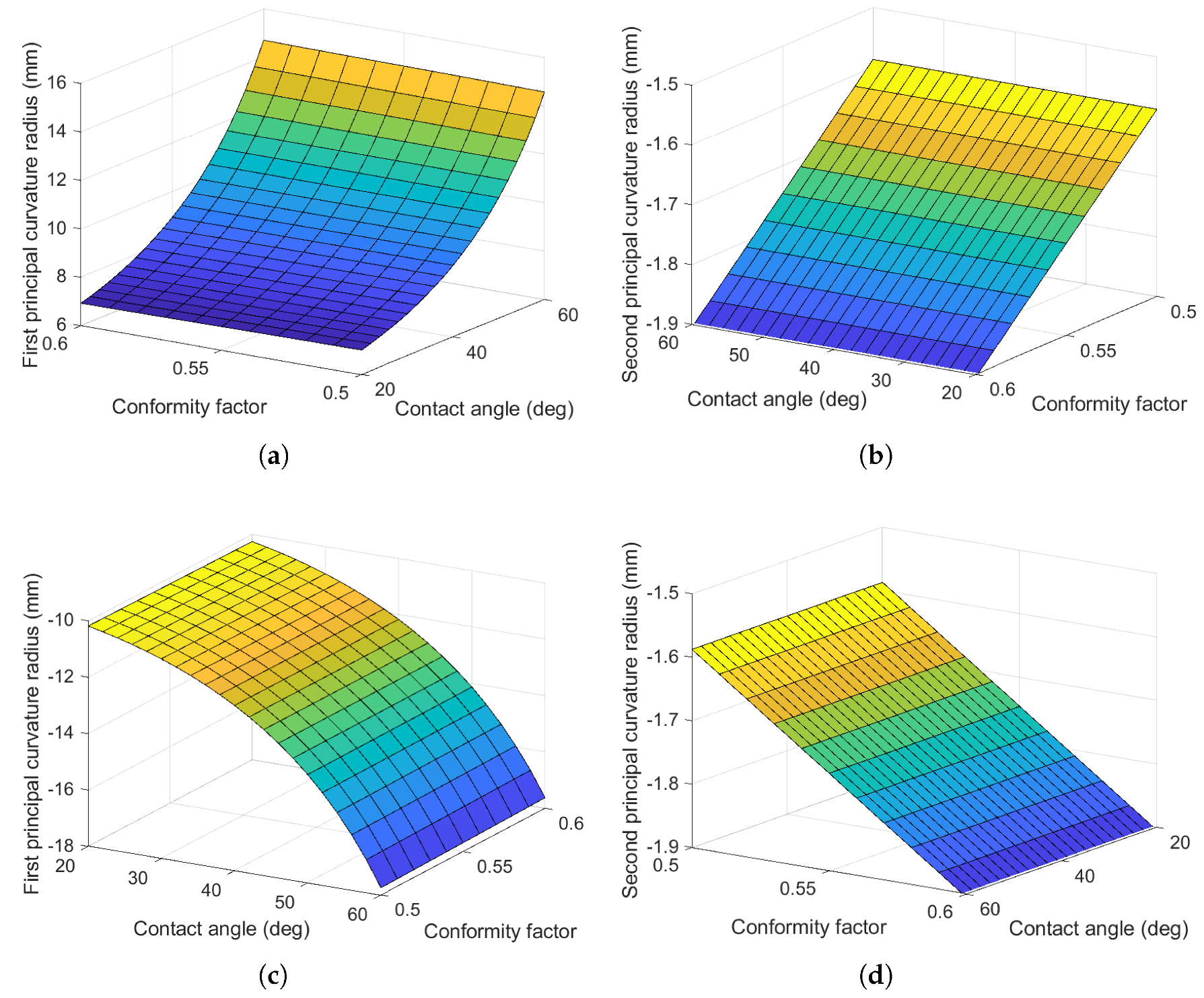
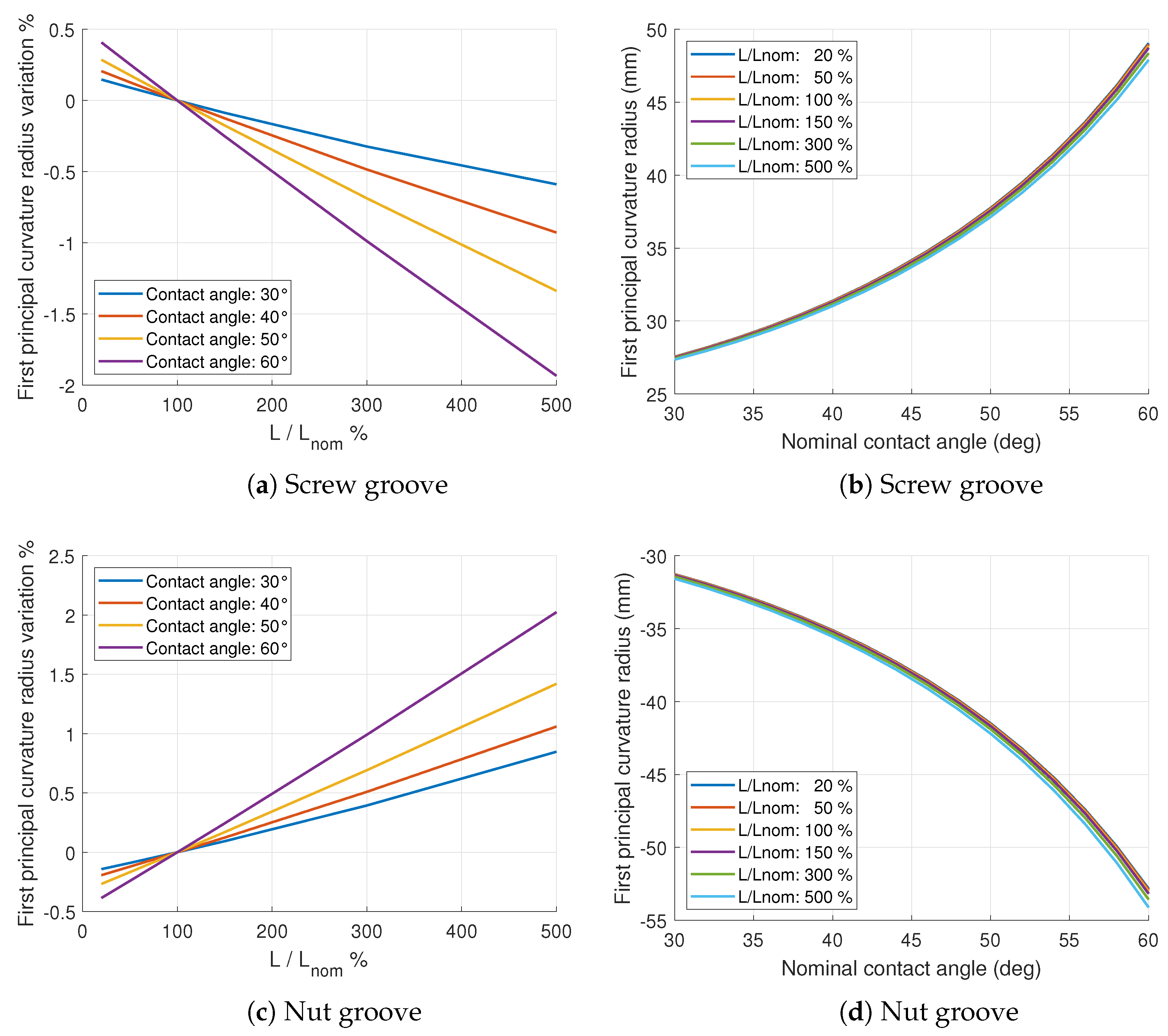
3. Results and Discussion

In this section, the dependences of the two principal curvature radii, defined as the inverse of the curvatures ${\kappa }_{1,2}$, with respect to the main constructive parameters are presented for the grooves of both the screw shaft and the nut. The first principal curvature is defined as the curvature of $\gamma$ on the plane $\mathsf{\Pi }$ (referring to Figure 3), while the second principal curvature is that of the groove profile on the $n-b$ plane (Figure 2).

Figure 5 shows the first principal curvature radius of the screw shaft and the nut grooves as a function of the pitch circle radius $r_m$ and the helix angle ${\alpha }_e$, considering a constant contact angle of ${45}^{\circ }$. The second principal curvature radius does not depend on these parameters, since they do not influence the shape of the groove section, but only the helix shape. It can be seen that the first principal curvature radius is almost linearly dependent on the pitch circle radius, while it presents a non-linear dependence on the helix angle. The higher ${\alpha }_e$, the more marked the variation of the curvature radius with $r_m$. In fact, as the helix angle increases, the curve $\gamma$ on the groove, shown in Figure 3, stretches and rectifies, until, in the limit situation of a helix angle of ${90}^{\circ }$, it becomes a straight line, parallel to the ball screw symmetry axis and with a first principal curvature radius tending to an infinite value, as can be observed in Figure 5. As expected, the geometry of the screw shaft and the nut involves that the curvature radii are described by positive values for the screw shaft and negative ones for the nut. The highest absolute values of the curvature radius would arise for increasing helix angles and pitch circle radii, for both the screw shaft and nut grooves.

The influence of the contact angle and the conformity factor on both the first and second principal curvature radii is shown in Figure 6. As already stated, the second principal curvature radius of both the screw shaft and the nut depends only on the raceway’s profile radius $r_s$ on the section normal to the thread. In fact, it can be seen in Figure 6b,d how it linearly depends on the conformity factor, according to Equation (2), while it is independent from the contact angle: its module increases with the conformity factor, assuming negative values because of the concavity of the raceway.

Conversely, the conformity factor has a minor influence on the first principal curvature radius (Figure 6a,c), which is, instead, non-linearly dependent on the contact angle. The higher the contact angle, the greater the curvature radius and, hence, the lower the curvature. Indeed, the identified point on the groove would lie on a larger helix as the contact angle increases, and would therefore have less torsion.

It can be observed that, while the values of the second curvature radius for the screw shaft and nut are the same, being dependent only on $r_s$, those of the first principal curvature radii are different not only in sign, but also in the module: this is because the nut groove is further than the screw shaft from the symmetry axis and, therefore, all the helices lying on its groove have grater base circle radii and minor curvatures.

The parameters L and H are responsible for the gothic shape of the groove profile and, as such, their value influence the principal curvatures of the raceways. However, as can be seen from Figure 7, their contribution on the absolute curvature value is very limited. Since according to Equations (3) and (4) the H and L parameters can be linked together by means of the theoretical contact angle ${\phi }_0$, the plots of Figure 7 show only the ogival offset L and the more intuitive theoretical contact angle ${\phi }_0$. Figure 7a depicts the variation of the first principal curvature value with respect to the non-dimensional parameter $L/L_{nom}$, representing the variation of the parameter with respect to its nominal value, and the contact angle for the screw shaft groove. The plot shows a clear linear dependency with the L parameter, which increases as the contact angle grows. When $L=L_{nom}$ all the curves intersect in the same point, correspondent to the trivial null variation.

The same results are represented switching the abscissa and legend parameter in Figure 7b, in which the evidently small influence of H and L on the global curvature value is evident. The same reasoning can be applied for the nut groove and similar results are shown in Figure 7c,d.

These observations corroborate the validity of the circular profile approximation made in Section 2.3 to obtain Equations (25) and (26) and the results presented thereafter.

Given a certain pitch circle radius $r_m$, two parameters play an important role in determining the first principal curvature radius value, i.e., the combination of the helix and the contact angle, as can be seen in Figure 8 by observing the red surfaces, denoted as “Exact” in the legends. The highest values can be obtained combining high helix angles and high contact angles. The dependence on the contact angle is stronger for high helix angles and vice versa. However, for low helix angle values the effect of the contact angle is limited, while, even for low contact angles, the helix angle still causes the first principal curvature radius to vary considerably. Figure 8a depicts the first principal curvature radius values for the screw shaft groove in the range $0^{\circ }$–${80}^{\circ }$ for both the contact and helix angles, while Figure 8b shows the first principal curvature radius of the nut groove versus the same parameters with identical ranges.

Figure 8 not only depicts the exact values but also shows the first principal curvature radius which would be obtained using the formulae present in the manufacturers’ catalogues and in the ISO3408 international standard [41], denoted as “Literature” in the legends. In fact, these literature formulae do not take into account any other constructive parameters except the contact angle, the pitch circle radius and the ball radius, disregarding the shape of the groove’s section and, especially, the helix angle, which has been shown be the most influential parameter. According to this formula, the first principal curvature radius of the screw shaft groove can be obtained as:

$$\frac{1}{{\kappa }_{1s,lit}}=\frac{r_m-r_{b}cos\left(\phi \right)}{cos\left(\phi \right)}$$

(27)

while that relative to the nut groove can be calculated through:

$$\frac{1}{{\kappa }_{1n,lit}}=-\frac{r_m+r_{b}cos\left(\phi \right)}{cos\left(\phi \right)}$$

(28)

These formulae directly derive from the bearing theory, in which the helix angle is null, and a circular groove profile is considered.

The results obtained with Equations (27) and (28) are shown in Figure 8 in violet: it can be clearly seen that only little variation with the contact angle is reproduced, although it is considerably far from the exact value, while the results are completely uncorrelated with the helix angle, as expected.

The comparison between the exact curvature values from the solution of Equation (24), the values obtained from the literature formulae (Equations (27) and (28)) and those calculated by means of the simplified equations (Equations (25) and (26)), varying the helix and contact angles, is shown in Figure 8a for the screw shaft and in Figure 8b for the nut grooves of a ball screw with $r_m=8$ mm, $r_b=1.5875$ mm, $H=0.0629$ mm and $L=0.0505$ mm. It can be seen that, for ${\alpha }_e\to 0$, the values obtained by the proposed formula, the literature formula and the exact solution converge to the same value, which is relative to a bearing. However, for increasing helix angles the literature solution does not accurately reproduce the real curvature radius values. Figure 9 depicts the relative errors committed by using both the proposed and the literature formulations, shown in the upper and lower graphs, respectively: it can be noted that the relative error for the literature formulation increases with the helix angle, while it does not show a significant dependence on the contact angle. On the other hand, the proposed formulation shows a mean relative error of 0.84% and a maximum relative error of <2.38% for the screw shaft curvature, and a mean relative error of 0.77% and a maximum relative error of <2.38%, for the nut curvature, over the domain $0^{\circ }$–${80}^{\circ }$ for both the contact and helix angles.

Normal ball screws have a contained helix angle, usually less than ${20}^{\circ }$, therefore the relative error committed using the literature formula result instead of the real value is in the order of 10–15%. Nevertheless, different typologies of ball screws exist for high speed applications, with helix angles of up to approximately ${45}^{\circ }$ ($r_m=12.5\mathrm{mm}$ and a lead of $80\mathrm{mm}$) or even more for custom constructive solutions: for these components, using the literature formula leads to a relative error of more than 50%, in contrast with a maximum of 2.38% with the proposed approach, which, in addition, shows far more reduced error for usually employed contact angle values. In fact, in order to maximize the mechanism’s efficiency, the contact angle is usually chosen by design as close to ${45}^{\circ }$: for these values, inspecting Figure 9, the relative error committed by using the proposed approximated formulation stays in the order of 1.3% or lower for the entire range of helix angles for both the screw shaft and nut grooves. Considering a contact angle of ${45}^{\circ }$, identified by the dashed red line in Figure 9, the maximum errors arise with extremely elevated helix angles: considering the range of common contact angles, i.e., <${40}^{\circ }$, the maximum error is lowered to 0.91% and 0.69% for the screw shaft and nut grooves respectively.

The proposed formulation was tested on different ball screw sizes usually present in manufacturers’ catalogues, applying the following procedure: for each size, defined by the nominal diameter, lead and ball diameter, 70 values of the curvature were calculated by using the exact, literature and proposed formulae, varying the contact angle in the range $0^{\circ }$–${70}^{\circ }$. The mean and maximum relative errors were obtained and recorded. Not all the results of the analysed 63 sizes of commercially available ball screws are listed in

Table A1. Relative errors on the screw shaft curvature committed by using the literature and proposed formulations for different off-the-shelf ball screws sizes, defined by the nominal diameter $D_{nom}$, the lead and the spheres’ diameter $D_b$.

${\mathrm{D}}_{\mathrm{nom}}$ (mm)	Lead (mm)	${\mathrm{D}}_{\mathrm{b}}$ (mm)	${\mathit{\alpha }}_{\mathit{e}}$ (deg)	Lit. ave./max. err. (%)	Proposed ave./max. err. (%)
125	10	7.144	1.46	0.30/0.31	0.24/0.24
160	25	12.7	2.85	0.60/0.61	0.33/0.34
125	20	12.7	2.92	0.71/0.73	0.43/0.45
160	30	12.7	3.42	0.71/0.73	0.33/0.34
125	25	12.7	3.64	0.87/0.89	0.43/0.44
125	30	12.7	4.37	1.06/1.09	0.43/0.44
100	30	12.7	5.45	1.54/1.60	0.54/0.57
80	25	12.7	5.68	1.81/1.90	0.70/0.73
125	40	12.7	5.82	1.54/1.58	0.42/0.44
80	30	9.525	6.81	2.04/2.12	0.50/0.52
63	25	9.525	7.20	2.42/2.53	0.65/0.68
50	20	6.35	7.26	2.30/2.39	0.53/0.56
100	40	12.7	7.26	2.30/2.39	0.53/0.56
32	15	6.35	8.49	3.43/3.65	0.87/0.94
50	25	6.35	9.04	3.25/3.37	0.52/0.55
32	20	6.35	11.25	5.30/5.63	0.82/0.90
80	60	9.525	13.43	6.35/6.57	0.44/0.47
25	20	3.5	14.29	7.29/7.59	0.51/0.56
40	40	6.35	17.66	10.89/11.39	0.52/0.60
32	32	4.762	17.66	10.77/11.23	0.49/0.56
50	60	6.35	20.91	14.29/14.78	0.35/0.42
32	40	4.762	21.70	15.60/16.23	0.40/0.49
63	80	7.144	22.01	15.50/15.96	0.29/0.36
40	60	6.35	25.52	21.01/21.86	0.33/0.45
40	60	7.144	25.52	21.36/22.34	0.38/0.52
25	50	3.5	32.48	31.45/32.41	0.14/0.26
32	64	4.762	32.48	31.63/32.66	0.15/0.28
50	100	7.144	32.48	31.51/32.49	0.14/0.27
20	50	3.5	38.51	42.42/43.82	0.15/0.54
20	65	3.5	43.68	51.39/52.81	0.27/0.84
25	80	3.5	45.53	53.80/54.90	0.27/0.76

for the screw shaft and in

Table A2. Relative errors on the nut curvature committed by using the literature and proposed formulations for different off-the-shelf ball screws sizes, defined by the nominal diameter $D_{nom}$, the lead and the spheres’ diameter $D_b$.

${\mathrm{D}}_{\mathrm{nom}}$ (mm)	Lead (mm)	${\mathrm{D}}_{\mathrm{b}}$ (mm)	${\mathit{\alpha }}_{\mathit{e}}$ (deg)	Lit. ave./max. err. (%)	Proposed ave./max. err. (%)
125	10	7.144	1.46	0.09/0.15	0.22/0.22
160	25	12.7	2.85	0.26/0.35	0.29/0.30
125	20	12.7	2.92	0.27/0.39	0.37/0.38
160	30	12.7	3.42	0.36/0.45	0.29/0.30
125	25	12.7	3.64	0.41/0.52	0.37/0.38
125	30	12.7	4.37	0.57/0.68	0.37/0.38
100	30	12.7	5.45	0.87/0.99	0.45/0.46
80	25	12.7	5.68	0.93/1.07	0.55/0.57
125	40	12.7	5.82	0.99/1.09	0.36/0.37
80	30	9.525	6.81	1.33/1.43	0.41/0.42
63	25	9.525	7.20	1.47/1.58	0.51/0.53
50	20	6.35	7.26	1.50/1.60	0.44/0.45
100	40	12.7	7.26	1.50/1.60	0.44/0.45
32	15	6.35	8.49	1.97/2.10	0.64/0.66
50	25	6.35	9.04	2.31/2.39	0.43/0.43
32	20	6.35	11.25	3.42/3.48	0.61/0.61
80	60	9.525	13.43	5.04/5.07	0.37/0.38
25	20	3.5	14.29	5.63/5.71	0.41/0.43
40	40	6.35	17.66	8.42/8.71	0.41/0.45
32	32	4.762	17.66	8.46/8.74	0.39/0.42
50	60	6.35	20.91	11.87/12.29	0.29/0.34
32	40	4.762	21.70	12.61/13.14	0.32/0.38
63	80	7.144	22.01	13.20/13.63	0.25/0.29
40	60	6.35	25.52	17.11/17.94	0.26/0.35
40	60	7.144	25.52	16.94/17.87	0.29/0.38
25	50	3.5	32.48	27.04/28.19	0.12/0.23
32	64	4.762	32.48	26.94/28.15	0.13/0.25
50	100	7.144	32.48	27.01/28.17	0.12/0.23
20	50	3.5	38.51	36.18/37.91	0.15/0.62
20	65	3.5	43.68	44.93/46.83	0.26/0.91
25	80	3.5	45.53	48.66/50.22	0.26/0.81

for the nut, because of space constraints. However, Figure 10a,b show the entire set of results.

It can be seen that, while the relative error committed by using the literature formulae increases with the helix angle, that of the proposed formulations remains approximately constant and is low. Furthermore, the average errors deriving from the proposed approximated equations should be considered when comparing the two types of results, since the maximum errors come from considering quite extreme contact angles (close to $0^{\circ }$ and ${70}^{\circ }$), while these values are usually not reached in real practice and the contact angle remains around the nominal contact angle [14,36]: for these values, close to ${45}^{\circ }$, the relative error is generally lower than $1\%$, as can also be observed in Figure 9. The proposed approximated solution gives an average relative error of 0.51% and an average relative error of 0.40% for the nut groove and the screw shaft groove on the whole dataset of ball screws. The enlarged areas in Figure 10a,b show that the error of the proposed formulae remains almost always below that of the literature formulation and, hence, this solution should be preferred.

It is interesting to note that the structure of the proposed formulae (Equations (25) and (26)) is quite similar to that of the literature equations (Equations (27) and (28)) except for the square cosine term related to the helix angle. Clearly, if possible, the exact solution should be preferred by using Equation (A1) or the two supplied MATLAB functions.

As stated in the introduction, the demonstrated increased accuracy of the new approximated formulation proposed in this work still keeps the computation time low, comparable to that of the existing literature formulation, while sensibly decreasing the relative error with respect to the exact solution. Figure 11 corroborates this statement showing the computational time histograms for the three approaches: the same calculation was repeated one million times on a 6-core Intel i7-10750H CPU (2.6 GHz) for each formulation, and the elapsed time was recorded. As expected, due to their extremely lower complexity, the approximated literature and proposed formulations took a mean of 0.249μs and 0.328μs respectively, against the 17.81μs of the exact solution, resulting in a 98% reduction. Assuming the model configuration presented in [14], i.e., a multibody simulation with a double nut preloaded ball screw with 30 spheres per nut, each one in contact with four circular half grooves (two of the screw shaft and two of the nut raceways), and considering a typical integration time step for stiff models of 1μs, the adoption of the proposed approximated solution instead of the exact solution leads to a saving of 11.6 h in a simulation of just 10 s. However, with small absolute values, the calculation times reduction allows maintaining high approximation accuracy with low computational effort.

4. Conclusions

In this paper the two principal curvatures of the grooves of the screw shaft and nut of a ball screw, considering a generic gothic arch profile of the thread normal section, were investigated. Hitherto, these values have been calculated by using the formulae for ball bearings, disregarding the helix angle and the profile parameters.

This article first introduced the exact formulae for the screw shaft and nut groove curvature evaluation, obtained following a rigorous differential geometry analytical approach: they were obtained by calculating the eigenvalues of the shape operator. The resulting equations were found to be quite long, complex and tricky to use. For this reason, two MATLAB functions have been made available as supplemental material for the readers.

In the case simpler expressions are needed, two new equations are proposed by assuming a circular profile groove and thus analytically simplifying the exact solution, in order to approximate the exact principal curvature radius values more accurately than with the commonly used literature formulae. It was shown that the first principal curvature radius values become larger with increasing pitch circle radii, helix angles and contact angles, i.e., with the increase of the distance from the ball screw axis. The major contributor to the first principal curvature radius growth was shown to be the helix angle. Therefore, the literature formulae, not considering it, lead to relative errors in the results which increase with this parameter, even up to more than 50%. On the other hand, the proposed approximate formulations present a mean relative error of approximately 0.51% and 0.40%, respectively, for the screw shaft and nut grooves, calculated on several constructive parameter combinations typical of commercially available off-the-shelf ball screws.

The proposed formulae are quite similar to the literature formula, easy to use and considerably more precise. While the usage of the exact formulation is always recommended when possible, the proposed equations represent a valid alternative for obtaining an accurate approximation of the exact curvature value. In particular, when high accuracy and low computation times are required, such as in high-fidelity models for prognostic activities and real-time applications, the proposed approximated solution guarantees a solution with a computational time comparable to actual widespread formulations, but at the same time with remarkably greater precision.

References

1. Simizu, S.; Sakato, K. Present Condition and Expectation for Ultra-precise Positioning Techniques from a Questionnaire. J. Jpn. Soc. Precis. Eng. 1995, 61, 1650–1655. [Google Scholar]
2. Altintas, Y.; Verl, A.; Brecher, C.; Uriarte, L.; Pritschow, G. Machine tool feed drives. CIRP Ann.—Manuf. Technol. 2011, 60, 779–796. [Google Scholar] [CrossRef]
3. Bertolaso, R.; Cheikh, M.; Barranger, Y.; Dupré, J.C.; Germaneau, A.; Doumalin, P. Experimental and numerical study of the load distribution in a ball-screw system. J. Mech. Sci. Technol. 2014, 28, 1411–1420. [Google Scholar] [CrossRef]
4. Chen, C.J.; Jywe, W.; Liu, Y.C.; Jwo, H.H. The development of using the digital projection method to measure the contact angle of ball screw. Phys. Procedia 2011, 19, 36–42. [Google Scholar] [CrossRef]
5. Levit, G. Recirculating ball screw and nut units. Mach. Tool. 1963, 34, 3–8. [Google Scholar]
6. Lin, M.C.; Ravani, B.; Velinsky, S.A. Kinematics of the Ball Screw Mechanism. J. Mech. Des. 1994, 116, 849–855. [Google Scholar]
7. Lin, M.C.; Velinsky, S.A.; Ravani, B. Design of the Ball Screw Mechanism for Optimal Efficiency. J. Mech. Des. 1994, 116, 856–861. [Google Scholar] [CrossRef]
8. Wei, C.C.; Lin, J.F. Kinematic Analysis of the Ball Screw Mechanism Considering Variable Contact Angles and Elastic Deformations. J. Mech. Des. 2003, 125, 717–733. [Google Scholar] [CrossRef]
9. Wei, C.C.; Lin, J.F.; Horng, J.H. Analysis of a ball screw with a preload and lubrication. Tribol. Int. 2009, 42, 1816–1831. [Google Scholar] [CrossRef]
10. Wei, C.C.; Lai, R.S. Kinematical analyses and transmission efficiency of a preloaded ball screw operating at high rotational speeds. Mech. Mach. Theory 2011, 46, 880–898. [Google Scholar] [CrossRef]
11. Xu, N.; Tang, W. Modeling and Analyzing the Slipping of the Ball Screw. Lat. Am. J. Solids Struct. 2015, 12, 612–623. [Google Scholar] [CrossRef]
12. Verl, A.; Frey, S. Correlation between feed velocity and preloading in ball screw drives. CIRP Ann.—Manuf. Technol. 2010, 59, 429–432. [Google Scholar] [CrossRef]
13. Zhou, C.G.; Feng, H.T.; Chen, Z.T.; Ou, Y. Correlation between preload and no-load drag torque of ball screws. Int. J. Mach. Tools Manuf. 2016, 102, 35–40. [Google Scholar] [CrossRef]
14. Bertolino, A.C.; Jacazio, G.; Mauro, S.; Sorli, M. Investigation on the ball screws no-load drag torque in presence of lubrication through MBD simulations. Mech. Mach. Theory 2021, 161, 104328. [Google Scholar] [CrossRef]
15. Cuttino, J.F.; Dow, T.A.; Knight, B.F. Analytical and Experimental Identification of Nonlinearities in a Single-Nut, Preloaded Ball Screw. J. Mech. Des. 1997, 119, 15. [Google Scholar] [CrossRef]
16. Kamalzadeh, A.; Gordon, D.J.; Erkorkmaz, K. Robust compensation of elastic deformations in ball screw drives. Int. J. Mach. Tools Manuf. 2010, 50, 559–574. [Google Scholar] [CrossRef]
17. Fukada, S.; Fang, B.; Shigeno, A. Experimental analysis and simulation of nonlinear microscopic behavior of ball screw mechanism for ultra-precision positioning. Precis. Eng. 2011, 35, 650–668. [Google Scholar] [CrossRef]
18. Horejs, O. Thermo-Mechanical Model of Ball Screw With Non-Steady Heat Sources. In Proceedings of the 2007 International Conference on Thermal Issues in Emerging Technologies: Theory and Application, Cairo, Egypt, 3–6 January 2007; pp. 133–137. [Google Scholar] [CrossRef]
19. Mauro, S.; Pastorelli, S.; Johnston, E. Influence of controller parameters on the life of ball screw feed drives. Adv. Mech. Eng. 2015, 7, 1–11. [Google Scholar] [CrossRef]
20. Mei, X.; Tsutsumi, M.; Tao, T.; Sun, N. Study on the load distribution of ball screws with errors. Mech. Mach. Theory 2003, 38, 1257–1269. [Google Scholar] [CrossRef]
21. Xu, S.; Yao, Z.; Sun, Y.; Shen, H. Load Distribution of Ball Screw with Consideration of Contact Angle Variation and Geometry Errors. In Proceedings of the IMECE2014, Montreal, Quebec, Canada, 14–20 November 2014; ASME: Montreal, QC, Canada, 2014; pp. 1–7, Volume 2B: Advanced Manufacturing. [Google Scholar] [CrossRef]
22. Okwudire, C.E. Reduction of torque-induced bending vibrations in ball screw-driven machines via optimal design of the nut. J. Mech. Des. Trans. ASME 2012, 134, 111008. [Google Scholar] [CrossRef]
23. Lin, B.; Okwudire, C.E. Low-Order Contact Load Distribution Model for Ball Nut Assemblies. SAE Int. J. Passeng. Cars—Mech. Syst. 2016, 9, 535–540. [Google Scholar] [CrossRef]
24. Oyanguren, A.; Larrañaga, J.; Ulacia, I. Thermo-mechanical modelling of ball screw preload force variation in different working conditions. Int. J. Adv. Manuf. Technol. 2018, 97, 723–739. [Google Scholar] [CrossRef]
25. Wen, J.; Gao, H.; Liu, Q.; Hong, X.; Sun, Y. A new method for identifying the ball screw degradation level based on the multiple classifier system. Meas. J. Int. Meas. Confed. 2018, 130, 118–127. [Google Scholar] [CrossRef]
26. Garinei, A.; Marsili, R. A new diagnostic technique for ball screw actuators. Meas. J. Int. Meas. Confed. 2012, 45, 819–828. [Google Scholar] [CrossRef]
27. Li, P.; Jia, X.; Feng, J.; Davari, H.; Qiao, G.; Hwang, Y.; Lee, J. Prognosability study of ball screw degradation using systematic methodology. Mech. Syst. Signal Process. 2018, 109, 45–57. [Google Scholar] [CrossRef]
28. Nguyen, T.L.; Ro, S.K.; Park, J.K. Study of ball screw system preload monitoring during operation based on the motor current and screw-nut vibration. Mech. Syst. Signal Process. 2019, 131, 18–32. [Google Scholar] [CrossRef]
29. Wei, C.C.; Liou, W.L.; Lai, R.S. Wear analysis of the offset type preloaded ball-screw operating at high speed. Wear 2012, 292–293, 111–123. [Google Scholar] [CrossRef]
30. Zhou, C.G.; Ou, Y.; Feng, H.T.; Chen, Z.T. Investigation of the precision loss for ball screw raceway based on the modified Archard theory. Ind. Lubr. Tribol. 2017, 69, 166–173. [Google Scholar] [CrossRef]
31. Bertolino, A.C.; De Martin, A.; Fasiello, F.; Mauro, S.; Sorli, M. A simulation study on the effect of lubricant ageing on ball screws behaviour. In Proceedings of the International Conference on Electrical, Computer, Communications and Mechatronics Engineering, ICECCME, Male, Maldives, 16–18 November 2022. [Google Scholar]
32. Liu, J.; Ma, C.; Wang, S. Precision loss modeling method of ball screw pair. Mech. Syst. Signal Process. 2020, 135, 106397. [Google Scholar] [CrossRef]
33. Braccesi, C.; Landi, L. A general elastic-plastic approach to impact analisys for stress state limit evaluation in ball screw bearings return system. Int. J. Impact Eng. 2007, 34, 1272–1285. [Google Scholar] [CrossRef]
34. Zhao, J.; Lin, M.; Song, X.; Jiang, H. Research on the precision loss of ball screw with short-time overload impact. Adv. Mech. Eng. 2018, 10, 1–9. [Google Scholar] [CrossRef] [Green Version]
35. Bertolino, A.C.; De Martin, A.; Mauro, S.; Sorli, M. Multibody dynamic ADAMS model of a ball screw mechanism with recirculation channel. In Proceedings of the IMECE, Virtual, 1–6 November 2021; pp. 1–10. [Google Scholar]
36. Bertolino, A.C.; Mauro, S.; Jacazio, G.; Sorli, M. Multibody Dynamic Model of a Double Nut Preloaded Ball Screw Mechanism With Lubrication. In Proceedings of the Volume 7B: Dynamics, Vibration, and Control; American Society of Mechanical Engineers: Portland, OR, USA, 2020; pp. 1–11. [Google Scholar] [CrossRef]
37. Bertolino, A.C.; Jacazio, G.; Mauro, S.; Sorli, M. Developing of a Simscape Multibody Contact Library for Gothic Arc Ball Screws: A Three-Dimensional Model for Internal Sphere/Grooves Interactions. In Proceedings of the IMECE, Salt Lake City, UT, USA, 11–14 November 2019; ASME, Ed.; American Society of Mechanical Engineers: Salt Lake City, UT, USA, 2019; pp. 1–8, Volume 4: Dynamics, Vibration, and Control. [Google Scholar] [CrossRef]
38. Bertolino, A.C.; De Martin, A.; Jacazio, G.; Sorli, M. A technological demonstrator for the application of PHM techniques to electro-mechanical flight control actuators. In Proceedings of the 2022 IEEE International Conference on Prognostics and Health Management (ICPHM), Detroit (Romulus), MI, USA, 6–8 June 2022; pp. 70–76. [Google Scholar] [CrossRef]
39. Bertolino, A.C.; De Martin, A.; Jacazio, G.; Mauro, S.; Sorli, M. Robust Design of a Test Bench for PHM Study of Ball Screw Drives. In Proceedings of the IMECE, Salt Lake City, UT, USA, 11–14 November 2019; ASME, Ed.; American Society of Mechanical Engineers: Salt Lake City, UT, USA, 2019; pp. 1–9, Volume 1: Advances in Aerospace Technology. [Google Scholar] [CrossRef]
40. Bertolino, A.C.; De Martin, A.; Gaidano, M.; Mauro, S.; Sorli, M. A fully sensorized test bench for prognostic activities on ball screws. In Proceedings of the 2021 International Conference on Electrical, Computer, Communications and Mechatronics Engineering (ICECCME), Port Louis, Mauritius, 7–8 October 2021; pp. 7–8. [Google Scholar] [CrossRef]
41. ISO 3408-1:2006; Ball Screws—Part 5: Static and Dynamic Axial Load Ratings and Operational Life. ISO: Geneva, Switzerland, 2006.
42. Meusnier, J. Mém. prés. par div. Etrangers. Acad. Sci. Paris 1785, 10, 477–510. [Google Scholar]
43. do Carmo, M.P. Differential Geometry of Curves and Surfaces, 2nd ed.; Dover Publications Inc.: Mineola, NY, USA, 2016. [Google Scholar]
44. Spivak, M. A Comprehensive Introduction to Differential Geometry, 3rd ed.; Publish or Perish Inc.: Houston, TX, USA, 1999; Volume 1. [Google Scholar]
45. MOOG. Ball Screws and Planetary Roller Screws; MOOG: Asheville, NC, USA, 2014. [Google Scholar]
46. NSK Corporation. Ball Screw Catalogue; NSK Corporation: Tokyo, Japan, 2021. [Google Scholar]
47. KSS. Ball Screws Catalogue; KSS: Tokyo, Japan, 2021. [Google Scholar]
48. Hiwin Corp. Ball Screws Catalogue; Hiwin Corp.: Taichung City, Taiwan, 2020. [Google Scholar]
49. Umbra Group. Industrial Ballscrews Catalogue; Umbra Group: Foligno, Italy, 2021. [Google Scholar]
Figure 1. A ball screw’s main reference systems.
Machines 11 00261 g001
Figure 2. Groove’s gothic arch profile of the (a) screw shaft and (b) nut on the n b plane of the Frenet–Serret reference frame.
Machines 11 00261 g002
Figure 3. Intersection of the (a) screw shaft and (b) nut grooves with the Π plane on which one of the two principal curvatures is calculated.
Machines 11 00261 g003
Figure 4. Procedure for obtaining the analytical and approximated formulae.
Machines 11 00261 g004
Figure 5. First principal curvature radius of the (a) screw shaft and (b) nut grooves depending on the pitch circle radius and the helix angle, for a ball screw with r b = 1.5875 mm, f s = 0.528 , φ = 45 deg, H = 0.0629 mm and L = 0.0505 mm.
Machines 11 00261 g005
Figure 6. First and second principal curvature radii of the (a,b) screw shaft and (c,d) nut grooves depending on the contact angle and the conformity factor, for a ball screw with r m = 8 mm, α e = 5.6806 deg, r b = 1.5875 mm, φ 0 = 45 deg.
Machines 11 00261 g006
Figure 7. First screw shaft and nut curvature variation with respect to the gothic arch parameter L (a,c) and to the nominal contact angle φ 0 (b,d) for a ball screw with r m = 25 mm, r b = 3.5 mm, p = 80 mm, φ 0 = 45 and H n o m = L n o m = 0.0693 mm.
Machines 11 00261 g007
Figure 8. Comparison between the first principal curvature radius exact values with the results of the proposed simplified formula and the literature formula for the (a) screw shaft and (b) nut grooves, for a ball screw with r m = 8 mm, r b = 1.5875 mm, H = 0.0629 mm and L = 0.0505 mm.
Machines 11 00261 g008
Figure 9. Relative errors committed by using the Eureqa solution (upper graphs) and the literature formula (lower graphs) on the first principal curvature radius of the (a) screw shaft and (b) nut grooves depending on the pitch circle radius and the helix angle, for a ball screw with r m = 8 mm, r b = 1.5875 mm, H = 0.0629 mm and L = 0.0505 mm.
Machines 11 00261 g009
Figure 10. Relative errors committed by using the Eureqa solution and the literature formula on the first principal curvature radius of the (a) screw shaft and (b) nut grooves for various off-the-shelf commercial ball screws, ordered against the helix angle (numerical results are listed in Table A1 and Table A2).
Machines 11 00261 g010
Figure 11. Calculation time histograms for the three formulations, for a ball screw with r m = 8 mm, r b = 1.5875 mm, p = 20 mm, φ = 45 deg, H = 0.0629 mm and L = 0.0505 mm.
Machines 11 00261 g011
Disclaimer/Publisher’s Note: The statements, opinions and data contained in all publications are solely those of the individual author(s) and contributor(s) and not of MDPI and/or the editor(s). MDPI and/or the editor(s) disclaim responsibility for any injury to people or property resulting from any ideas, methods, instructions or products referred to in the content.