
Equivalent Consumption Minimization Strategy of Hybrid Electric Vehicle Integrated with Driving Cycle Prediction Method
1
College of Electrical and Information Engineering, Hunan University, Changsha 410082, China
2
Hunan Lixing Power Technology Co., Ltd., Zhuzhou 412001, China
3
ThyssenKrupp Presta Fawer (Changchun) Co., Ltd., Changchun 130033, China
4
College of Automotive Engineering, Jilin University, Changchun 130022, China
*
Author to whom correspondence should be addressed.
Machines 2023, 11(6), 576; https://doi.org/10.3390/machines11060576
Submission received: 23 April 2023
/
Revised: 16 May 2023
/
Accepted: 19 May 2023
/
Published: 23 May 2023
(This article belongs to the Special Issue Energy Management and ECO-Driving Strategies of Hybrid Electric Vehicles)
Abstract
:Hybrid electric vehicles that can combine the advantages of traditional and new energy vehicles have become the optimal choice at present in the face of increasingly stringent fuel consumption restrictions and emission regulations. Range-extended hybrid electric vehicles have become an important research topic because of their high energy mixing degree and simple transmission system. A compact traditional fuel vehicle is the research object of this study and the range-extended hybrid system is developed. The design and optimization of the condition prediction energy management strategy are investigated. Vehicle joint simulation analysis and bench test platforms were built to verify the proposed control strategy. The vehicle tracking method was selected to collect real vehicle driving data. The number of vehicles in the field of view and the estimation of the distances between the front and following vehicles are calculated by means of the mature algorithm of the monocular camera and by computer vision. Real vehicle cycle conditions with driving environment and slope information were constructed and compared with all driving data, typical working conditions under NEDC, and typical working conditions under UDDS. The BP neural network and fuzzy logic control were used to identify the road conditions and the driver’s intention. The results showed that the equivalent fuel consumption of the control strategy was lower than that of the fixed-point power following control strategy and vehicle economy improved.
1. Introduction
New energy vehicles are usually vehicles driven entirely, or mainly, by new forms of energy. These vehicles have received extensive research attention from various countries and institutes because of their adoption of a new type of power system with high efficiency, low emissions, and low pollution. Hybrid electric vehicles utilize two or more energy storage systems that mainly use internal combustion engines and motors as power sources. The advantages and disadvantages of energy management strategies determine the overall performance of the vehicle. Therefore, the energy management strategy of the power system has been extensively investigated. The energy management strategy aims to control the energy flow between different power sources of the power train according to the power demands of the vehicle. A reasonable management strategy can optimize the potential of the power system and reduce energy consumption and emission pollution. Energy management strategies are mainly divided into rule-, optimization- and learning-based techniques [1,2,3].
The logic of the rule-based management strategy is to collect information, such as driving speed, power demand of the vehicle, and battery power, whilst the vehicle is being driven. The corresponding rule threshold logic table usually set for the upper and lower limits of driving motor speed, engine torque constraints, and power battery state of charge can be subdivided into two categories: deterministic and fuzzy rules [4,5,6]. Jalil N et al. [7] proposed a rule-based control strategy that selects three variables: power demand, driver’s acceleration command, and battery state of charge. The engine and battery work as efficiently as possible to improve the economy of the vehicle through appropriate power and torque distribution. Kim M et al. [8] proposed a hybrid thermostat strategy for series hybrid electric vehicles. This new thermostat approach combines the advantages of the power follower strategy to achieve high efficiency. The optimization-based management strategy can be divided into two categories: global and real-time optimization. The optimized management strategy can solve the multi-objective and constrained nonlinear optimization problem of the hybrid power system and achieve optimal performance under different driving conditions [9,10,11,12,13]. Satoshi et al. [14] explored an effective energy management system, which optimized the operating area of the internal combustion engine, and proposed a torque control strategy for parallel hybrid electric vehicle battery charging to sufficiently reduce the emission of harmful pollutants. Erfan et al. [15] designed a new and efficient engine start–stop control method and adopted a self-learning optimization algorithm to optimize the working point of the internal combustion engine under different driving conditions and to remarkably reduce the fuel consumption of the vehicle under different cycle conditions. M.S. Teja et al. [16] used the particle swarm optimization algorithm to optimize the fuel consumption, power output, and energy flow of hybrid electric vehicles. A comparison of guidelines proved that the method rapidly completed the design and reduced fuel consumption and vehicle emissions. With the development of artificial intelligence and the improvement of computing performance, learning-based methods have attracted the attention of many scholars [17,18,19]. Wang et al. [20] proposed a HEV method integrated with an ORC (HEV–ORC) using reinforcement learning. The simulation results showed that DRL-based EMS can save 2% more fuel energy than rule-based EMS. Cheng et al. [21] put forward an energy management strategy based on real-time update reinforcement learning to allocate the energy flow of the hybrid system reasonably under unknown conditions.
The complex and changeable working environments of vehicles when driving on the road include objective road facilities and real-time traffic conditions. If a vehicle is in a congested section of a road, then, from the perspective of optimizing the vehicle’s control strategy, the facts that the road traffic flow is large, the speed is slow, and the starts and stops are frequent need to be taken into account. Under these conditions, the economy of the vehicle should be prioritized by not running the engine at low speed for a long time, avoiding frequent engine starts and stops, and using pure electric driving as extensively as possible. If a vehicle is on a smooth road for a long time, then it is likely that the traffic flow on the road is less and the speed is high. The driving range of the vehicle should be taken into account so as to ensure the engine works efficiently and to provide sufficient backup power for the vehicle. However, actual road conditions present high uncertainty, and determining the driving conditions of vehicles using traditional methods is difficult. Therefore, existing energy management strategies of vehicles fail to achieve predetermined energy saving and emission reduction effects in actual use. If road condition identification and vehicle driving condition prediction can be carried out, then the engine, generator, motor, power battery, and other components can be reasonably controlled so as to effectively reduce vehicle exhaust emissions and energy loss.
Research on vehicle condition prediction is mainly divided into two categories: known and unknown driving conditions [22,23,24]. The known driving cycle refers to the driving process on a fixed route. Real-time information is not used in the actual research process. The control strategy offering minimum fuel consumption during the entire driving process is investigated on the basis of given typical cycle conditions and historical information. To assess unknown future driving conditions, current driving information for the vehicle, combined with certain perceptive means to assist in identifying road conditions and predicting future driving conditions, are necessary. This kind of investigation has gradually become an important research direction with enrichment of perceptual means gaining attention in recent years because of its importance and feasibility in engineering practice.
Yue Wang et al. [25] conducted an in-depth analysis of driving information from both historical and future dimensions, completed cycle construction and future driving prediction, and proposed a hierarchical optimization control strategy based on driving information. Erik et al. [26] used GPS and a route slope database to complete road slope predictive control. Real vehicle GPS information combined with the database was applied to determine the location of the vehicle, complete the vehicle’s predictive control, and improve the vehicle’s 3.5% fuel saving rate. Jun Hou et al. [27] proposed an optimal energy management strategy, based on vehicle–cloud connection, that considers battery decay and electricity cost and uses the dynamic programming method on the cloud computing platform. The model predictive control method is used to deal with uncertainty constraints of the system. The simulation results showed the superiority of the method with an improvement rate of 40%, compared with the rule-based method. The analysis demonstrated that research on traditional driving cycle identification is based on the existing typical driving cycle and real vehicle historical driving information [28,29,30]. The vehicle’s perception of the surrounding environment has improved with the development of intelligent vehicles. Research on the predictive control of a vehicle’s driving cycle under an unknown driving cycle will be applied to real vehicles in the future [31,32].
The future driving state of a vehicle has strong randomness and no posteriority (i.e., the state of the previous moment has no direct influence on the driving state of the next moment), which are Markov characteristics. The Markov chain is widely used in natural science and engineering technology, and is effective in state prediction. Therefore, many researchers use the Markov algorithm to conduct research into the prediction of working conditions [33,34]. In the actual driving process of a vehicle, it is usually impossible to achieve predetermined energy saving and emission reduction effects. If road condition identification and vehicle driving condition prediction can be carried out, the engine, generator, motor, power battery and other components can be controlled more reasonably, which can effectively reduce vehicle exhaust emission and reduce vehicle energy loss. In contrast to an energy management strategy that integrates vehicle networking information, the main contribution of this paper is the improved control strategy gained through prediction of future driving conditions of a vehicle by means of the vehicle ‘s own sensors, and integration into the ECMS strategy of this improved road condition recognition method with the driver intention recognition strategy through the utilization of fuzzy logic. In this way, the ECMS strategy has a predictive energy management function. The main idea of the fusion is to adjust the SOC threshold and the vehicle demand power in the ECMS control strategy. The results showed that it can effectively improve the economy of the vehicle.
This paper is organized as follows. An approach based on control of the predictive equivalent consumption minimization strategy (ECMS) under unknown conditions is proposed in the first part this study. The research object and modeling method of a hybrid electric vehicle are briefly introduced in the second part. The identification of road conditions and driver intentions suitable for the algorithm are identified and integrated into the ECMS algorithm in the third part. Finally, a test bench is built in the fourth part to verify the algorithm.
2. Hybrid Electric Vehicle Model Construction
2.1. Drive Motor System Model
The driving motor is the power source of driving vehicles with two outputs of torque and power at work. The motor and motor controller are usually considered as a whole when modeling. A theoretical model of the motor was established to analyze the voltage of each winding of the motor with electromagnetic torque characteristics as the output. Considering the simple mechanical structure and fast torque response of the motor, an experimental model of the motor, combined with the control demand of the hybrid system, met simulation requirements. The motor test bench is shown in Figure 1.
According to the experimental model, the expected output torque of the motor is as follows:
where, is the peak torque of the motor at speed; α is the torque load rate, is the motor speed.
2.2. Equivalent Circuit Model
In this paper, the equivalent circuit method was used to construct the power battery model. The equivalent circuit modeling method describes the performance of the power battery by establishing an ordinary differential equation. It is assumed that the battery is composed of circuit components, such as capacitance, resistance, and voltage source. This method greatly simplifies the complexity of modeling. The equivalent internal resistance model is a relatively simple model, which ignores the polarization characteristics of the battery and has low accuracy. On this basis, the Thevenin model increases the polarization resistance and polarization capacitance of the battery, and the simulation accuracy of the working state of the battery is high [35].
The state of charge (SOC ) of the battery represents the percentage of the remaining power of the battery to the total power, which is affected by many factors, such as battery temperature, life, charge and discharge speed. The of the battery can be calculated by the current, the value at the previous moment and the total capacity using the ampere–hour integration method:
where, is the of the battery; is the of the battery at the previous moment; is the ampere–hour capacity of the battery.
2.3. Reducer Model
The forward transmission of the reducer can reduce the speed and increase the output torque, so as to provide sufficient wheel driving power, and reversely transmit power during braking recovery. In this paper, the modeling process mainly considered longitudinal dynamics, without considering the differential, and the transmission distance was not long. It was assumed that the transmission shaft was rigid, and that the reducer adopted a cylindrical gear reducer. The expressions of wheel end torque , speed and moment of inertia of the reducer are as follows:
where, is the reducer motor end torque; is the mechanical efficiency of the reducer; is the speed of the reducer motor end; is the reducer motor end equivalent rotational inertia; is the rotary inertia of the reducer. Among these values, is affected by the transmission direction.
2.4. Engine Model
The engine itself has a complex structure, such as a crank connecting rod and valve system, and has many auxiliary systems, such as cooling and lubrication. The working process involves strong transient processes, such as ventilation and combustion. The modeling of this part is always difficult. Common modeling methods include the steady-state test model, the average value model and the theoretical model. This paper selected the steady-state experimental model to construct the model’s engine, which met simulation requirements. The model includes an engine controller, which takes speed, throttle opening and the start-stop command as inputs and outputs engine torque and fuel consumption rate.
According to the input speed table, the zero opening torque and the full opening torque of the throttle are obtained, and the engine torque output is preliminarily estimated by using the throttle opening :
where, and are the minimum and maximum torques at engine speed; is the throttle opening. The friction torque loss of the engine at each speed is measured by the power analyzer, and the actual engine output torque is corrected:
Engine output power and average effective pressure are divided into:
where 9550 denotes the unit conversion factor, denotes the engine torque.
The fuel consumption rate and total fuel consumption of the engine are calculated as follows:
where, denotes the effective power and Be denotes the average effective fuel consumption rate obtained by using the fuel consumption meter with the dynamometer.
2.5. Vehicle Model
This paper focused on the power and economy of the vehicle, so the model mainly considered the longitudinal dynamics of the vehicle, that is, the mathematical relationship between the longitudinal force and the motion of the vehicle. In the stable state, the dynamic equation of the resistance of the vehicle is:
where, is the total resistance of the vehicle; is the road rolling resistance; is the slope resistance; is the air resistance; is the accelerating resistance; is the vehicle full load quality; is the rolling resistance coefficient; is the ramp angle; is the acceleration of gravity; is the wind resistance coefficient; is the windward area of the vehicle; is the rotating mass conversion coefficient for the vehicle.
3. Method and Simulation
This section mainly proposes road condition identification and driving intention recognition suitable for the ECMS strategy. The algorithm’s structure is shown in Figure 2. In the first half of this section, an improved method of road condition identification and improved driver intention recognition strategy, based on fuzzy logic, are introduced. In Section 3.2 and Section 3.3, the strategy of integrating the predictive features with the ECMS method and the corresponding verification are addressed.
3.1. Road Condition Identification and Driving Intention Recognition
3.1.1. Improvement of Road Condition Identification Based on Neural Network Method
The degree of congestion in driving conditions is of great significance to the energy management system of hybrid vehicles. Traditional driving conditions are categorized according to traffic conditions or driving areas, such as urban conditions, suburban conditions, and high-speed conditions. Based on vehicle driving history information, the neural network is utilized to divide the number of vehicles in a field of view, and to determine driving conditions for each time period as being congested, neutral or unobstructed.
The artificial neural network is an intelligent mathematical method, which can simulate the logical reasoning ability of the human brain and is suitable for dealing with complex pattern recognition problems. The BP (Back Propagation) neural network is the most commonly used method to establish a mapping relationship through input and output parameters provided by training samples, and adjusts the error back propagation for network training. In the design process of the BP neural network, the number of hidden layers greatly influences the mapping ability and generalization ability of the system. This paper studied the identification of driving road conditions. The output was divided into three categories: congestion, neutral and unobstructed. The following three types of working conditions correspond to the vector form outputs: congestion condition [1,0,0]; neutral condition [0,1,0]; smooth condition [0,0,1]. The selected neural network had 11 input parameters and 3 output parameters.
The number of nodes is determined according to the following empirical formula:
where the number of input parameters is 11, is the number of output parameters and x can be any constant between 0 and 11.
A BP neural network system of 11 × 10 × 3 was built in this study. Parameters, such as training function, are listed in Table 1.
The error distribution, mean square error, gradient and regression number obtained by training the BP neural network are shown in Figure 3, Figure 4, Figure 5 and Figure 6, respectively.
In order to verify the rationality of the number of vehicles in the field of view introduced by the network, a neural network with only 10 driving parameters and a neural network with 11 input parameters were trained. The results were used to identify real vehicle experimental conditions. The results of the two-road condition identification are shown in Figure 7. It can be seen from the diagram that most of the two different road condition identification networks were accurately identified. The method of using the BP neural network to identify the road condition of the cycle condition is very feasible.
A subjective evaluation method was used to ignore the transition stage of the working condition, and the total identification accuracies of each working condition were 78.9% and 89.5%, respectively. Compared with an identification method that introduces monocular visual information, an identification method that does not use the number of vehicles in the field of view experiences a certain degree of misidentification. In Figure 7b, in graph period 121–180 s, it can be observed that the traditional identification method identified the working condition as neutral, while the improved identification result of the corresponding period, as seen in the graph in Figure 7c, identified congestion. It was speculated that the reason the traditional road condition identification process mistakenly identified conditions as neutral was based on the driving speed and vehicle acceleration action, with a maximum speed of more than 40 km/h, at this stage. From the number of vehicle detections in the field of view, it can be seen that the numbers of vehicles were mostly 4 or 5, and the result was corrected to more realistic driving conditions.
In Figure 7b, graph time period 601–720 s, the traditional identification method identified the working condition as congestion, while the improved identification of the corresponding time period in Figure 7c graph identified it as neutral. An analysis of the vehicle speed diagram showed that there was a long idle condition in this section, which corresponded to a waiting situation at a traffic intersection in the actual driving process. The traditional identification method took into account factors such as lower average speed and mileage in the working section and misjudged the identification results as being congestion. In the improved identification results, the number of vehicles in the field of view was mostly represented as neutral conditions. There were 3 or 4 vehicles, not significantly different from the aforementioned neutral working section, and the identification results were corrected to neutral. From the perspective of the working condition section, the improved BP neural network had a more accurate identification effect in dealing with the two types of working conditions of rapid acceleration and long idle speed in the working condition section.
3.1.2. Improved Driving Intention Recognition Based on Fuzzy Logic
Driving intention mainly includes acceleration, braking and cruising, and it is realized by the accelerator pedal and the brake pedal. Since driving intention is closely related to vehicle operation conditions, the real-time traffic environment and the driver’s psychology, acceleration and deceleration pedal opening is greatly affected by a driver’s personal operational habits, and real-time performance is high. With this in mind, i is difficult to adopt an accurate mathematical model or mathematical language definition, so fuzzy control was adopted. The basic structure of the fuzzy controller includes four main parts: knowledge base, fuzzy interface, fuzzy inference engine and anti-fuzzy interface.
The defuzzification interface contains defuzzification steps. The fuzzy results obtained by reasoning need to be defuzzified and divided into quantitative output control values. The center of gravity method is the most commonly used method. The final output control value is obtained by weighting the output fuzzy quantities according to the membership degree.
3.1.3. Analysis of Intention Recognition Results
The results of driving intention recognition during driving are shown in Figure 8a. It can be seen from the diagram that the designed recognition system better identified the driver’s intention to accelerate and decelerate the vehicle. By comparing with the driving speed, as shown in Figure 8a, the environmental parameter of the change rate of the vehicle distance was introduced, so that there was earlier identification of the driver’s intention than the vehicle’s start time, and some working conditions were even identified earlier than the driver’s pedal operation. Compared with the traditional method of intention recognition, using only vehicle information such as speed and accelerator pedal, the predictability greatly improved.
In order to evaluate the recognition results, it is assumed that the recognition result at time t is , and whether the vehicle acceleration is consistent with the action of the intention recognition result is judged within . If it is consistent, it is regarded as a precise recognition, and if it is not, it is regarded as a false recognition. The proportion of precise recognition number to total recognition number is defined as the recognition accuracy. According to the statistics, the accuracy of total of 1380 s experimental cycle recognition was 85.3%. Figure 8b shows the input parameters and recognition result diagram of the 0–300 s stroke. It can be seen from the diagram that the main reason for the recognition error was the input parameters of the driver’s pedal. The pedal opening range was large and there were many membership functions. The second reason was that the driver needed to tread on the brake pedal for a long time when stopping at idle speed, and the acceleration intention judgment was delayed when starting again.
3.2. Threshold Condition Prediction Optimization
Combined with the results of road identification and driver intention recognition, the traditional ECMS control strategy was adjusted as follows:
- Under congestion conditions, the vehicle starts and stops frequently, but the power demand is not high. At this time, if the SOC reaches the preset , the CS mode is turned on to start the range extender to start power generation, and the surplus power is used for power battery charging. At the end of driving, the power battery surplus is too high. Long-term driving in congestion conditions also means the range extender frequently starts and stops. By reducing the threshold, the above situation can be improved. The control strategy was set as follows: was adjusted to 27% and was adjusted to 30% when the driver’s intention was not to accelerate quickly in congested conditions.
- Under the neutral condition, the parameter remained unchanged at 30%, and the was adjusted to 33%;
- When the SOC does not reach the preset , the CS mode is opened in advance and the range extender is at the lowest point of specific fuel consumption to generate electricity, to avoid long-term operation of the engine at high speed and low efficiency, and, thereby, to meet driving demands, improve the overall economy of the vehicle and contribute to improving high-speed driving mileage. The above situation can be improved by increasing the threshold. The control strategy was set as follows: was adjusted to 33% and was adjusted to 36% when the driver’s intention was not to decelerate at the current time.
The predictive SOC adaptive ECMS (PS–ECMS) strategy and the engine fixed point and power following (FPPF) strategy were compared through simulation under real vehicle experimental conditions.
Figure 9 shows the comparison of SOC simulation curves of the power battery under the FPPF and PS–ECMS strategies. In the first half of the simulation, the battery SOC of the FPPF strategy rose from 30% to about 35%, the post-control strategy actively closed the range extender, and the battery SOC curve also decreased. When the SOC of the 940 s battery reached 30%, it reopened, and, finally, dropped to 34.2% after 1320 s of closing. The PS–ECMS strategy rapidly decreased the battery SOC at the beginning of the simulation, which began to rise when it reached 27.6% at 359 s. The battery SOC was maintained at about 30% in the neutral road condition section, and the battery SOC rose sharply to 32.6% after 1051 s.
Affected by the change of vehicle driving power and charging power, the SOC curves of the two groups of batteries indicated local jitter. When the battery was charged, the two sets of curves at some operating points (such as at 1100 s, 1170 s) showed a decrease in power, indicating that the power generated by the range extender was less than the required power of the vehicle, and the vehicle was in mixed drive mode. The average demand power of the vehicle under the unobstructed condition was higher, and the battery charging speed was slower than at other time periods. At the same time, the instantaneous high demand power frequency of the vehicle under the unobstructed condition was higher, so the number of charging state power drops after 1000 s increased.
From the comparison of the battery SOC curves obtained by the FPPF and PS–ECMS strategies, it can be clearly observed that the SOC curve of the FPPF strategy battery had faster fluctuation speed and larger upper and lower range values. However, under different working conditions, the SOC curves of PS–ECMS were stable near the preset lower limit, and the change of the value also affected the range of the SOC curves. Although the overall upper and lower ranges were also large, the SOC ranges were maintained in the range of 3.5% under different working conditions. The PS–ECMS strategy was beneficial to the charging and discharging efficiencies and to the service life of the power batteries. The SOC at the end of the FPPF strategy could be any value between and , while the PS–ECMS strategy stabilized the SOC at a lower target value at the end of the trip, which was more economical.
Figure 10 illustrates the comparison of the total fuel consumption simulation curves of the engine under the FPPF and PS–ECMS strategies. Under the FPPF strategy, engine fuel consumption rose roughly along a straight line between 0–273 s and 939 s–1320 s, and the rest of the time it remained unchanged. The final fuel consumption was 867.7 g, and there were several fast-rising segments in the straight line. At this stage, the engine deviated from the lowest point of specific fuel consumption due to the power following strategy. The PS–ECMS strategy began to consume fuel at 360 s, showing a stepped rise, and the final fuel consumption was 786.3 g. Compared with the FPPF strategy, the PS–ECMS strategy considered both the low-power and high-power driving requirements of the vehicle, and the curvature of the fuel consumption curve changed, but the slope difference when the curve rose is not large, indicating that the operating point was basically near the lowest point of specific fuel consumption. The total fuel consumption of the PS–ECMS strategy at the end of the trip was significantly lower than that of the FPPF strategy.
Figure 11 shows the comparison of engine speed simulation curves under the FPPF and PS–ECMS strategies. The FPPF strategy had two operation intervals. The engine speed in the 0–273 s interval was basically at the lowest point of 2000 rpm fuel consumption, and the power demand was higher at some time points. After the engine speed rose, it returned quickly. The vehicle demand power was higher in the unobstructed working condition, so the engine speed deviated from 2000 revolutions more frequently in 939 s–1320 s. The operation interval of the PS–ECMS strategy was relatively scattered, and the speed of each operation interval was basically near the lowest point of specific fuel consumption.
In summary, the PS–ECMS control strategy effectively reduced the battery power at the end of the trip and improved the economy under different road conditions. The energy consumption parameters of the two control strategies are shown in Table 2. From the table, it can be concluded that the equivalent fuel consumption of the PS–ECMS control strategy reduced by 4.45%.
3.3. Vehicle Demand Power Input Value Condition Prediction Optimization
The ECMS control strategy is based on real-time driving demand power generating the power for the range extender. Compared with the traditional control strategy, it can improve economy and reduce fuel consumption. However, during the simulation of the PS–ECMS strategy, the range extender started 7 times in 1380 s. In actual driving, it is necessary to consider the problem of slow power supply if the battery power is low but the driver has rapid acceleration demand. The driver would sense a traditional fuel vehicle with idle start and stop functions. When driving starts again at an intersection there is a rapid acceleration demand, and the vehicle’s power output is extremely slow. This phenomenon is similar to the possible consequences of frequent starts and stops of the ECMS control strategy extender. In this section, future vehicle demand power is corrected by introducing the driving intention, identified in Section 3.1’s condition prediction, so as to optimize the vehicle demand power input value of the ECMS control strategy. In this way, the range extender can generate electricity according to future power demand.
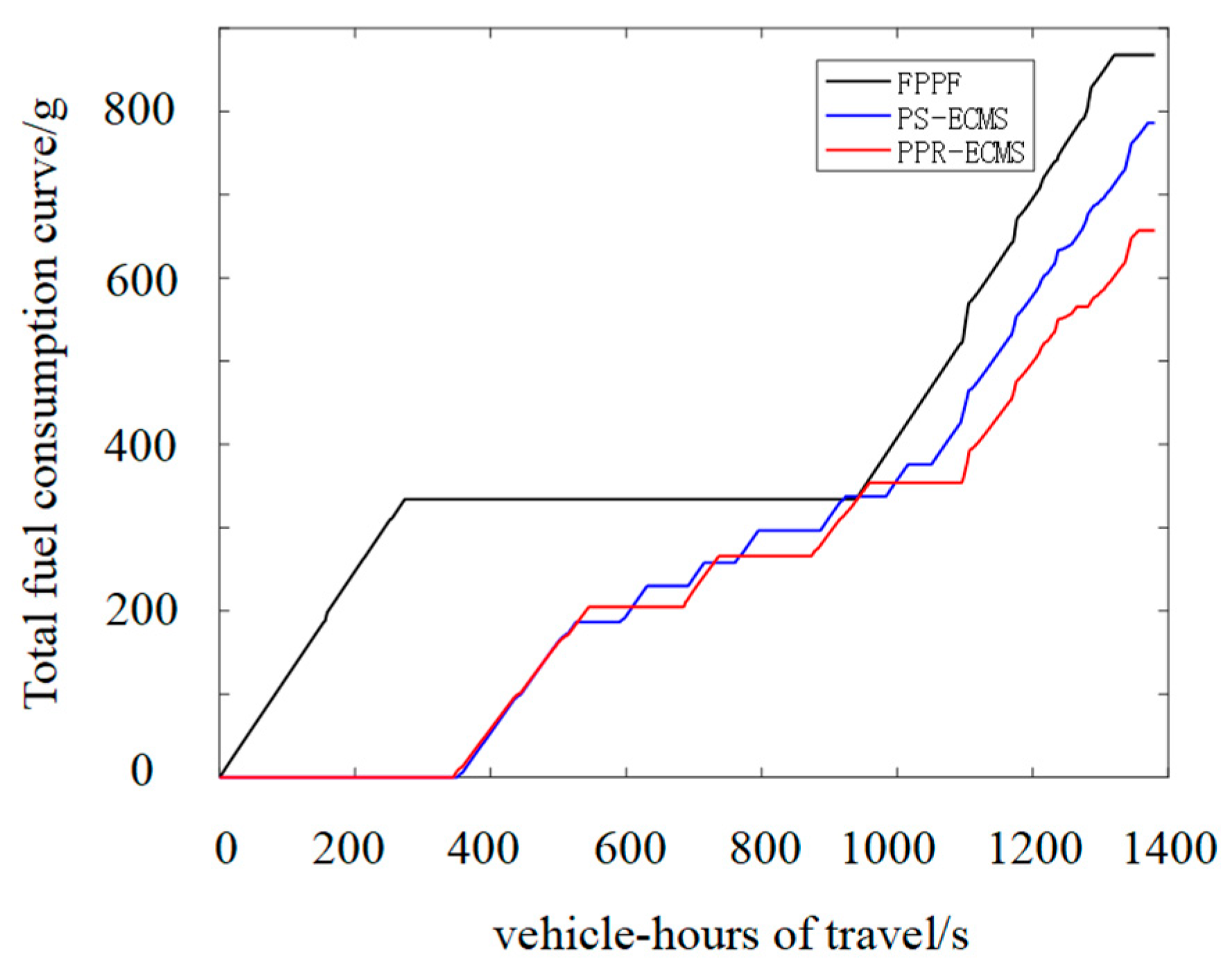
The PS–ECMS control strategy was adjusted as follows. The proportional coefficient of the vehicle demand power in the ECMS control strategy was modified according to the driver’s intention. The driver’s intention was to increase vehicle demand power during acceleration and rapid acceleration. The driver’s intention was to keep the vehicle demand power constant when the speed was uniform. The driver’s intention was to reduce the vehicle demand power during deceleration and rapid deceleration. The proportional coefficients were defined as 1.2, 1.1, 1.0, 0.9 and 0.8, respectively. The predictive power request adaptive ECMS (PPR–ECMS) strategy was compared with the engine fixed-point + power following strategy. Figure 12, Figure 13 and Figure 14 provide the simulation curves of the power battery SOC, engine total fuel consumption and engine speed under FPPF, PS–ECMS and PPR–ECMS strategies, respectively.
The dynamic SOC curve of the improved control strategy (Figure 12) was more susceptible to the demand power. Therefore, the charging oscillation amplitude of the battery SOC was higher than that of PS–ECMS. Under the 450 s–900 s neutral working condition, the FPPF and PS–ECMS strategies had time points (577 s, 746 s) when the power decreased and the vehicle urgently needed power. The PPR–ECMS strategy could precharge the battery based on the larger demand power predicted by the driver’s intention, so that the power generated by the extender was transmitted to the drive motor through the high-voltage bus the first time. When the vehicle was driving at high speed in unobstructed road sections, the driving intention recognition was maintained at a constant speed and deceleration for a long time. Therefore, the PPR–ECMS strategy tended to consume more electricity, so the battery SOC was kept in a lower range. The final value of the battery SOC reduced to 31.5% at the end of the stroke, which was lower than that of the normal setting under unobstructed conditions. The reason was that there were more deceleration and rapid deceleration driving intentions identified in the unobstructed road section, and the upper and lower thresholds of the SOC were adjusted to the original value. This indicated that the PPR–ECMS strategy helped to reduce the SOC of the battery at the end of the stroke.
In regard to the total fuel consumption curve of the engine (Figure 13), the start-up time of the PPR–ECMS strategy was similar to that of the PS–ECMS strategy, and the initial fuel consumption was slightly higher than that of the PS–ECMS strategy. There was little difference in fuel consumption under the neutral working condition, and the fuel consumption in the unobstructed working condition was significantly lower than in the other two strategies. It was evident that at medium and high speed, the PPR–ECMS strategy, combined with the driver’s driving intention, offered better economy and avoided the vehicle charging too much power at high speed.
The engine speed curve (Figure 14), compared with the PS–ECMS curve, indicated that the PPR–ECMS strategy had a longer running time during the start-up period, avoiding the three starts and stops of the extender near 590 s, 760 s, and 983 s. The control goal of reducing the number of starts and stops was successfully achieved. During the operation of the engine, the speed fluctuation range significantly improved compared with the FPPF and PPR–ECMS strategies. The peak speed reached 6000 rpm, and there were many working conditions below 2000 rpm, which might damage the power battery life and cause vehicle vibration. It also required high responsiveness when the generator torque follows.
In summary, the PPR–ECMS control strategy predicted the future vehicle demand power through the driver’s intention, and could significantly reduce the start and stop times of the range extender in neutral/unobstructed road conditions, but the operation range of the range extender changes greatly. The energy consumption parameters of the three control strategies are shown in Table 3 From the table, it can be concluded that the equivalent fuel consumption of the PPR-ECMS strategy was 1.08% higher than that of PS–ECMS and 5.48% higher than that of FPPF.
4. Bench Test Verification
4.1. Extender System Test Bench Construction
In order to verify the corresponding control strategy, a bench test wass built for analysis. The test bench mainly includes two motors and motor controllers, engines, eddy current dynamometers, dynamometer control systems, fuel consumption meters, rapid prototyping controllers, battery simulation test systems, power analyzers and other components. With the existing equipment conditions in the laboratory, the bench test platform of the range extender system was built, as shown in Figure 15. The powertrain performance test bench structure schematic diagram is shown in Figure 16. The main test equipment models used in the figure are shown in Table 4. As the control unit of the whole system, the rapid prototyping controller receives the signals from the motor controller, the engine controller, the battery simulation test system, the fuel consumption meter and the power analyzer through the CAN bus, and automatically generates the code according to the designed energy management strategy. The battery simulation test system simulates the power battery pack and provides voltage, current, SOC and other information. The power analyzer can be used to measure the input and output power and working efficiency of the motor.
The PPR–ECMS control strategy needs to dynamically calculate the required power of the vehicle in combination with the driver’s intention. Since the driver’s intention recognition changes rapidly, and considering the computing power of the rapid prototyping controller equipment in the bench test, only the PS–ECMS strategy test was carried out for verification. In addition, when the ECMS strategy optimized the optimal operating point of the required power, in order to save computing resources, the equivalent fuel of the range extender under different power generation powers was calculated from 5 kW to 50 kW with a gradient of 5 kW, and the minimum power point of the equivalent fuel taken.
4.2. Analysis of Bench Test Results
The neutral condition segments with time periods of 430–1080 s were extracted from the real vehicle experimental cycle, and the bench experiments of FPPF and PS–ECMS energy management strategies were carried out, respectively. When conducting two sets of control strategy tests, the data of the dynamometer control system, power analyzer, battery simulation test system, fuel consumption meter and other equipment in the bench were recorded or transmitted and saved, and the battery power consumption and engine fuel consumption calculated. The numerical results of equivalent fuel consumption per hundred kilometers are summarized in Table 5.
It can be seen from the energy consumption table that, compared with the FPPF control strategy, the operation time of the PS–ECMS range extender was significantly lower. Similar to the simulation strategy, the PS–ECMS strategy tended to generate power and stop as soon as possible.
There were three start-stop times of the PS–ECMS strategy in the simulation time of 650 s, which was not conducive to the performance of power response and emission. In terms of 100 km equivalent fuel consumption, the equivalent fuel consumption of the PS–ECMS strategy was 3.816% higher than that of the FPPF strategy, which was lower than the improvement of simulation economy. The reasons may be as follows: 1. In the simulation model, the engine model could not simulate the dynamic response process well, ignoring the low fuel consumption caused by partial energy loss; 2. Limited by the optimal power gradient setting of the test bench, the actual operating point of the range extender was not the best point at the time used in the simulation.
In summary, after bench test verification, the PPR–ECMS control strategy effectively improved the economy of the range extender, and the equivalent fuel consumption per hundred kilometers reduced by 3.816% compared with the fixed-point power following strategy.
5. Conclusions and Discussion
In this paper, a compact traditional fuel vehicle was taken as the research object, and the optimization of energy management strategy for condition prediction studied. The main research content includes the following: parameter design of power train components, construction of REEV joint simulation analysis platform; construction of real vehicle driving cycle with driving environment, road condition identification and driving intention recognition, construction of an improved ECMS control strategy based on driving cycle prediction, simulation analysis and experimental verification. The specific research content follows:
- (1)
- Based on vehicle performance requirements in different modes, the parameters of the power train components were designed. The energy flow under the four working modes of REEV was analyzed. In the CD and CS modes, combined with the performance requirements of the vehicle, the selection and parameter matching of the drive motor, power battery, reducer, engine and generator were completed according to the three levels of extreme working condition design, acceleration capacity design and efficiency optimization design.
- (2)
- A real vehicle driving cycle with environmental information was constructed and the driving cycle prediction carried out.
Real vehicle driving data were collected, and a mature open-source algorithm used to complete the vehicle number identification and the front and following distance measurements for the video stream in the front field of view obtained by the monocular camera. An experimental cycle condition, with environmental information, was constructed. The comprehensive parameter value of the experimental cycle condition was 0.223, which represented the driving data of the original vehicle. The BP neural network and fuzzy logic control were used to complete the identification of road conditions and driver’s intention recognition, respectively. The accuracy of road condition identification, based on the number of vehicles in the field of view, was 10.6% higher. The driving intention recognition, based on the distance between following vehicles, accelerated the recognition time on the basis of ensuring an accuracy of 85.3%, and the overall recognition prediction was better.
- (3)
- An improved ECMS energy management strategy, based on condition prediction, was developed. The ECMS model was established under battery charging and discharging conditions. The equivalent factor and the average power value of braking energy recovery in the model were set according to identification of different road conditions. The SOC threshold and the demand power of the vehicle were adjusted according to the prediction results. The PS–ECMS and PPR–ECMS control strategies were built and simulated. The results showed that the control strategy improved the economy of the vehicle compared with the fixed-point power following control strategy, and the equivalent fuel consumption per 100 km reduced by 4.45% and 5.48%, respectively.
In the future, we will conduct a neural network-based work condition prediction mechanism analysis and explore the influential factors between neural network parameters and work condition prediction. From the current feasibility analysis, it appears that integrating the vehicle’s own sensors into driver assistance or energy management strategies is both convenient and feasible, and can be implemented in practice. While it is true that Vehicle-to-Vehicle (V2V) communication is a promising technology for improving road safety and traffic efficiency, the use of camera-based systems for detecting and analyzing the behavior of vehicles in front is also a common approach in many advanced driver assistance systems (ADAS). That being said, V2V communication can also provide valuable information about the behavior and intentions of other vehicles, especially in situations where visual detection is limited, such as in adverse weather conditions or obstructed views. Therefore, a combination of camera-based systems and V2V communication could potentially provide the best of both worlds, and it is likely that future ADAS will incorporate both technologies for enhanced safety and efficiency.
Author Contributions
Methodology, X.Z. and Q.H.; Validation, D.N., C.Y. and X.Z.; Investigation, C.Y.; Resources, X.Z. and F.S.; Data curation, C.Y.; Writing—original draft, D.N.; Writing—review & editing, D.L.; Visualization, D.N. All authors have read and agreed to the published version of the manuscript.
Funding
This work was supported in part by the National Key R&D Program of China under Grant 2021YFB2500703.
Data Availability Statement
Not applicable.
Conflicts of Interest
The authors declare no conflict of interest.
References
- Du, G.; Zou, Y.; Zhang, X.; Guo, L.; Guo, N. Heuristic Energy Management Strategy of Hybrid Electric Vehicle Based on Deep Reinforcement Learning with Accelerated Gradient Optimization. IEEE Trans. Transp. Electrif. 2021, 7, 2194–2208. [Google Scholar] [CrossRef]
- Rabinowitz, A.; Araghi, F.M.; Gaikwad, T.; Asher, Z.D.; Bradley, T.H. Development and Evaluation of Velocity Predictive Optimal Energy Management Strategies in Intelligent and Connected Hybrid Electric Vehicles. Energies 2021, 14, 5713. [Google Scholar] [CrossRef]
- Zhang, F.; Wang, L.; Coskun, S.; Pang, H.; Cui, Y.; Xi, J. Energy Management Strategies for Hybrid Electric Vehicles: Review, Classification, Comparison, and Outlook. Energies 2020, 13, 3352. [Google Scholar] [CrossRef]
- Li, J.-Q.; Fu, Z.; Jin, X. Rule Based Energy Management Strategy for a Battery/Ultra-capacitor Hybrid Energy Storage System Optimized by Pseudospectral Method. Energy Procedia 2017, 105, 2705–2711. [Google Scholar] [CrossRef]
- Li, X.; Han, L.; Liu, H.; Wang, W.; Xiang, C. Real-time optimal energy management strategy for a dual-mode power-split hybrid electric vehicle based on an explicit model predictive control algorithm. Energy 2019, 172, 1161–1178. [Google Scholar] [CrossRef]
- Peng, J.; He, H.; Xiong, R. Rule based energy management strategy for a series–parallel plug-in hybrid electric bus optimized by dynamic programming. Appl. Energy 2016, 185 Pt 2, 1633–1643. [Google Scholar] [CrossRef]
- Jalil, N.; Kheir, N.A.; Salman, M. A rule-based energy management strategy for a series hybrid vehicle. In Proceedings of the 1997 American Control Conference, Albuquerque, NM, USA, 4–6 June 1997; pp. 689–693. [Google Scholar]
- Kim, M.; Jung, D.; Min, K. Hybrid Thermostat Strategy for Enhancing Fuel Economy of Series Hybrid Intracity Bus. IEEE Trans. Veh. Technol. 2014, 63, 3569–3579. [Google Scholar] [CrossRef]
- Li, P.; Sheng, W.; Duan, Q.; Li, Z.; Zhu, C.; Zhang, X. A Lyapunov Optimization-Based Energy Management Strategy for Energy Hub with Energy Router. IEEE Trans. Smart Grid 2020, 11, 4860–4870. [Google Scholar] [CrossRef]
- Lü, X.; Wu, Y.; Lian, J.; Zhang, Y. Energy management and optimization of PEMFC/battery mobile robot based on hybrid rule strategy and AMPSO. Renew. Energy 2021, 171, 881–901. [Google Scholar] [CrossRef]
- Sellali, M.; Ravey, A.; Betka, A.; Kouzou, A.; Benbouzid, M.; Djerdir, A.; Kennel, R.; Abdelrahem, M. Multi-Objective Optimization-Based Health-Conscious Predictive Energy Management Strategy for Fuel Cell Hybrid Electric Vehicles. Energies 2022, 15, 1318. [Google Scholar] [CrossRef]
- Wang, X. Parameters Optimization of Hybrid Powertrain Based on Optimization Energy Management Strategy. Bus Coach. Technol. Res. 2018, 11–13. [Google Scholar]
- Wang, X.; Huang, Y.; Guo, F.; Zhao, W. Energy Management Strategy based on Dynamic Programming Considering Engine Dynamic Operating Conditions Optimization. In Proceedings of the 2020 39th Chinese Control Conference (CCC), Shenyang, China, 27–29 July 2020. [Google Scholar] [CrossRef]
- Kitayama, S.; Saikyo, M.; Nishio, Y.; Tsutsumi, K. Torque control strategy incorporating charge torque and optimization for fuel consumption and emissions reduction in parallel hybrid electric vehicles. Struct. Multidiscip. Optim. 2016, 54, 177–191. [Google Scholar] [CrossRef]
- Taherzadeh, E.; Dabbaghjamanesh, M.; Gitizadeh, M.; Rahideh, A. A New Efficient Fuel Optimization in Blended Charge Depletion/Charge Sustenance Control Strategy for Plug-in Hybrid Electric Vehicles. IEEE Trans. Intell. Veh. 2018, 3, 374–383. [Google Scholar] [CrossRef]
- Teja, M.; Varma, P.S.; Irfan, M.; Sudarshan, E. Designing for Control Strategy by Particle Swarm Optimization in Parallel Hybrid Electric Vehicles for Economical Fuel Consumption. IOP Conf. Series Mater. Sci. Eng. 2020, 981, 042034. [Google Scholar] [CrossRef]
- Qi, C.; Zhu, Y.; Song, C.; Yan, G.; Xiao, F.; Zhang, X.; Cao, J.; Song, S. Hierarchical reinforcement learning based energy management strategy for hybrid electric vehicle. Energy 2022, 238, 121703. [Google Scholar] [CrossRef]
- Qi, C.; Song, C.; Xiao, F.; Song, S. Generalization ability of hybrid electric vehicle energy management strategy based on reinforcement learning method. Energy 2022, 250, 123826. [Google Scholar] [CrossRef]
- Qi, C.; Zhu, Y.; Song, C.; Cao, J.; Xiao, F.; Zhang, X.; Xu, Z.; Song, S. Self-supervised reinforcement learning-based energy management for a hybrid electric vehicle. J. Power Sources 2021, 514, 230584. [Google Scholar] [CrossRef]
- Wang, X.; Wang, R.; Shu, G.; Tian, H.; Zhang, X. Energy management strategy for hybrid electric vehicle integrated with waste heat recovery system based on deep reinforcement learning. Sci. China Technol. Sci. 2021, 65, 713–725. [Google Scholar] [CrossRef]
- Cheng, Y.; Xu, G.; Chen, Q. Research on Energy Management Strategy of Electric Vehicle Hybrid System Based on Reinforcement Learning. Electronics 2022, 11, 1933. [Google Scholar] [CrossRef]
- Liu, Q.; Dong, S.; Yang, Z.; Xu, F.; Chen, H. Energy Management Strategy of Hybrid Electric Vehicles Based on Driving Condition Prediction-ScienceDirect. IFAC-PapersOnLine 2021, 54, 265–270. [Google Scholar] [CrossRef]
- Wang, X.; Wang, Q. An Energy Management Method of Electric Vehicles Based on Stochastic Model Predictive Control. Basic Clin. Pharmacol. Toxicol. 2019, 124, 350. [Google Scholar]
- Xu, J.; Alsabbagh, A.; Ma, C. Prediction-Based Game-Theoretic Strategy for Energy Management of Hybrid Electric Vehicles. IEEE J. Emerg. Sel. Top. Ind. Electron. 2022, 3, 79–89. [Google Scholar] [CrossRef]
- Wang, Y.; Zeng, X.; Song, D. Hierarchical optimal intelligent energy management strategy for a power-split hybrid electric bus based on driving information. Energy 2020, 199, 117499. [Google Scholar] [CrossRef]
- Hellström, E. Look-Ahead Control of Heavy Trucks Utilizing Road Topography. Ph.D. Thesis, Institutionen för Systemteknik, Linköping, Sweden, 2007. [Google Scholar]
- Hou, J.; Song, Z. A hierarchical energy management strategy for hybrid energy storage via vehicle-to-cloud connectivity. Appl. Energy 2020, 257, 113900. [Google Scholar] [CrossRef]
- Deng, T.; Zhao, K.; Yu, H. An adaptive equivalent consumption minimization strategy considering catalyst temperature for plug-in hybrid electric vehicle. Proc. Inst. Mech. Eng. Part D J. Automob. Eng. 2022, 236, 1375–1389. [Google Scholar] [CrossRef]
- Qiu, L.; Qian, L.; Zomorodi, H.; Pisu, P. Design and optimization of equivalent consumption minimization strategy for 4WD hybrid electric vehicles incorporating vehicle connectivity. Sci. China Technol. Sci. 2018, 61, 147–157. [Google Scholar] [CrossRef]
- Rezaei, A.; Burl, J.B.; Zhou, B. Estimation of the ECMS Equivalent Factor Bounds for Hybrid Electric Vehicles. IEEE Trans. Control. Syst. Technol. 2017, 26, 2198–2205. [Google Scholar] [CrossRef]
- Serrao, L.; Onori, S.; Rizzoni, G. ECMS as a realization of Pontryagin’s minimum principle for HEV control. In Proceedings of the 2009 American Control Conference, St. Louis, MO, USA, 10–12 June 2009. [Google Scholar]
- Sezer, V.; Gokasan, M.; Bogosyan, S. A Novel ECMS and Combined Cost Map Approach for High-Efficiency Series Hybrid Electric Vehicles. IEEE Trans. Veh. Technol. 2011, 60, 3557–3570. [Google Scholar] [CrossRef]
- Hatherall, O.; Marco, J.; Barari, A.; Niri, M.F. Load Prediction Based Remaining Discharge Energy Estimation Using a Combined Online and Offline Prediction Framework. In Proceedings of the 2022 IEEE Conference on Control Technology and Applications (CCTA), Trieste, Italy, 23–25 August 2022; pp. 1196–1201. [Google Scholar] [CrossRef]
- Hatherall, O.; Niri, M.F.; Barai, A.; Li, Y.; Marco, J. Remaining discharge energy estimation for lithium-ion batteries using pattern recognition and power prediction. J. Energy Storage 2023, 64, 107091. [Google Scholar] [CrossRef]
- He, Y.; Li, Q.; Zheng, X.; Liu, X. Equivalent hysteresis model based SOC estimation with variable parameters considering temperature. J. Power Electron. 2021, 21, 590–602. [Google Scholar] [CrossRef]
Figure 1.
Motor test bench.

Figure 2.
The structure of this paper’s algorithm.

Figure 3.
BP neural network error histogram.

Figure 4.
BP neural network mean square deviation diagram. The intersection point is the best verification performance point.
Figure 4.
BP neural network mean square deviation diagram. The intersection point is the best verification performance point.

Figure 5.
BP neural network gradient diagram.

Figure 6.
BP neural network regression figure.

Figure 7.
Comparison of real vehicle road condition identification results. (a) is the vehicle driving cycle. (b) is the number of vehicles in the no field of view, and (c) is the number of vehicles in the field of view.
Figure 7.
Comparison of real vehicle road condition identification results. (a) is the vehicle driving cycle. (b) is the number of vehicles in the no field of view, and (c) is the number of vehicles in the field of view.

Figure 8.
Fuzzy driver intention recognition results. (a) 0–1380 s identification results. (b) 0–300 s identification results.
Figure 8.
Fuzzy driver intention recognition results. (a) 0–1380 s identification results. (b) 0–300 s identification results.

Figure 9.
Power battery SOC curve comparison.

Figure 10.
Comparison of engine fuel consumption curves.

Figure 11.
Engine speed curve simulation comparison.

Figure 12.
Power battery SOC curve simulation comparison.

Figure 13.
Simulation comparison of engine total fuel consumption curve.

Figure 14.
Simulation comparison of engine speed curve.

Figure 15.
Range extender system bench physical map.

Figure 16.
Powertrain performance test bench structure schematic diagram.


Table 1.
BP neural network parameter table.
| Type | Parameter |
|---|---|
| the number of hidden layers | 1 |
| number of the hidden layer nodes | 10 |
| hidden layer transfer function | logsig |
| Output layer transfer function | tansig |
| training function | trainlm |
| performance index | minimum mean square error (MSE) |
| learning goal | 1 × 10⁻⁶ |
| the number of hidden layers | 1 |
Table 2.
Comparison of Energy Consumption between FPPF and PS-ECMS.
| Control Strategy | FPPF | PS-ECMS |
|---|---|---|
| Initial SOC/% | 30 | 30 |
| Final value SOC/% | 34.2 | 33.5 |
| power consumption/kWh | −0.652 | −0.544 |
| power consumption/g | 867.7 | 786.3 |
| Equivalent oil consumption/(L/100 km) | 5.841 | 5.581 |
Table 3.
Comparison of Energy Consumption FPPF, PS-ECMS and PPR-ECMS.
| Control Strategy | FPPF | PS-ECMS | PPR-ECMS |
|---|---|---|---|
| Initial SOC/% | 30 | 30 | 30 |
| Final value SOC/% | 34.2 | 33.5 | 31.5 |
| power consumption/kWh | −0.652 | −0.544 | −0.187 |
| power consumption/g | 867.7 | 786.3 | 656.9 |
| equivalent oil consumption/(L/100 km) | 5.841 | 5.581 | 5.521 |
Table 4.
Range extender system bench main test equipment model table.
| Item | Model |
|---|---|
| Electric eddy current dynamometer | China, CAMA CW-260 |
| Dynamometer control system | China, CAMA FST-4 |
| power analyzer | Japan, YOKOGAWA WT-1800 |
| Battery simulation test system | Avi, AVL e-Storage |
| fuel consumption meter | China, FCM-1 |
| Coolant constant temperature device | China, SHW-300 |
Table 5.
Bench test energy consumption table of different control strategies.
| Test Condition | Real Vehicle Experiment Cycle | |
|---|---|---|
| control strategy | FPPF | PS-ECMS |
| power consumption/kWh | −0.375 | −0.304 |
| oil consumption/g | 333.531 | 320.363 |
| starting and stopping times | 1 | 3 |
| Operation time of range extender/s | 274 | 233 |
| equivalent oil consumption/(L/100 km) | 6.865 | 6.603 |
Disclaimer/Publisher’s Note: The statements, opinions and data contained in all publications are solely those of the individual author(s) and contributor(s) and not of MDPI and/or the editor(s). MDPI and/or the editor(s) disclaim responsibility for any injury to people or property resulting from any ideas, methods, instructions or products referred to in the content. |
© 2023 by the authors. Licensee MDPI, Basel, Switzerland. This article is an open access article distributed under the terms and conditions of the Creative Commons Attribution (CC BY) license (https://creativecommons.org/licenses/by/4.0/).
Share and Cite
MDPI and ACS Style
Ni, D.; Yao, C.; Zheng, X.; Huang, Q.; Luo, D.; Sun, F. Equivalent Consumption Minimization Strategy of Hybrid Electric Vehicle Integrated with Driving Cycle Prediction Method. Machines 2023, 11, 576. https://doi.org/10.3390/machines11060576
AMA Style
Ni D, Yao C, Zheng X, Huang Q, Luo D, Sun F. Equivalent Consumption Minimization Strategy of Hybrid Electric Vehicle Integrated with Driving Cycle Prediction Method. Machines. 2023; 11(6):576. https://doi.org/10.3390/machines11060576
Chicago/Turabian StyleNi, Dacheng, Chao Yao, Xin Zheng, Qing Huang, Derong Luo, and Farong Sun. 2023. "Equivalent Consumption Minimization Strategy of Hybrid Electric Vehicle Integrated with Driving Cycle Prediction Method" Machines 11, no. 6: 576. https://doi.org/10.3390/machines11060576
Note that from the first issue of 2016, this journal uses article numbers instead of page numbers. See further details here.