
An Improved Automation System for Destructive and Visual Measurements of Cross-Sectional Geometric Parameters of Microdrills

Department of Mechanical and Mechatronic Engineering, National Taiwan Ocean University, Keelung 20224, Taiwan
*
Author to whom correspondence should be addressed.
Machines 2023, 11(6), 581; https://doi.org/10.3390/machines11060581
Submission received: 12 April 2023
/
Revised: 13 May 2023
/
Accepted: 14 May 2023
/
Published: 23 May 2023
(This article belongs to the Special Issue Industrial Process Improvement by Automation and Robotics)
Abstract
:Microdrills are specific cutting tools widely used to drill microholes and microvias. For certain microdrill manufacturers, a conventional sampling inspection procedure is still manually operated for carrying out the destructive and visual measurements of two essential cross-sectional geometric parameters (CSGPs), called the cross-sectional web thickness (CSWT) and the cross-sectional outer diameter (CSOD), of their straight (ST) and undercut (UC) type microdrill products. In order to comprehensively automate the conventional sampling inspection procedure, a destructive and visual measuring system improved from an existing vision-aided automation system, for both the hardware and the automated measuring process (AMP), is presented in this paper. The major improvement of the hardware is characterized by a machine vision module consisting of several conventional machine vision components in combination with an innovative and lower cost optical subset formed by a set of plano-concave achromatic (PCA) lenses and a reflection mirror, so that the essential functions of visually positioning the drilltip and visually measuring the CSGPs can both be achieved via the use of merely one machine vision module. The major improvement of the AMP is characterized by the establishment of specific image processing operations for an auto-focusing (AF) sub-process based on two-dimensional discrete Fourier transform (2D-DFT), for a web thickness measuring (WTM) sub-process based on an iterative least-square (LS) circle-fitting approach, and for an outer diameter measuring (ODM) sub-process based on integrated applications of an iterative LS circle-fitting approach and an LS line-fitting-based group-dividing approach, respectively. Experiments for measuring the CSGPs of microdrill samples were conducted to evaluate the actual effectiveness of the developed system. It showed that the developed system could achieve good repeatability and accuracy for the measurements of the CSWTs and CSODs of both ST and UC type microdrills. Therefore, the developed system could effectively and comprehensively automate the conventional sampling inspection procedure.
1. Introduction
Microdrilling processes, based on mechanical and laser microdrilling techniques, have been widely adopted by printed circuit board (PCB) industries for the mass production of microholes and microvias in single- and multi-layer PCBs [1,2,3]. Mechanical microdrilling is based on the fundamentals of conventional cutting processes [4,5,6,7,8,9,10,11,12,13,14,15,16] and the use of specific cutting tools called microdrills to drill microholes and microvias. As compared with laser microdrilling, higher hole quality and lower equipment cost are the advantages of mechanical microdrilling, although such a conventional cutting process may also lead to slightly lower positioning accuracy and drilling efficiency. Therefore, microdrills are necessary and high-demand consumables for PCB industries, and superior design, rapid and precision manufacture, and reliable inspection techniques must be involved for their mass production.
Nowadays, commercially available microdrill products can be classified into the straight (ST) and undercut (UC) type microdrills, as shown by the illustrations depicted in Figure 1. Each type of microdrill can be functionally divided into two main portions: the drill body and the shank. (Note that for the purpose of clarity of illustration, the drill body of each microdrill depicted in Figure 1 is exaggerated.) The drill body, usually with a nominal diameter under 0.5 mm, can be further functionally divided into two sub-portions: the drill point and the helical flutes. The drill point, with the geomety of a so-called four-facet chisel point [2,4,5], is designed to produce cutting action inside the PCB (i.e., the workpiece). The helical flutes are designed to provide screw-shaped passageways for chip removal. The main difference between the ST and UC type microdrills is that the drill body of an ST type one has a diametral continuity along its axial direction, but that of a UC type one has a diametral discontinuity occurring at a certain axial location. The drill body of a UC type microdrill, besides its front portion adjacent to the drill point, is further ground to yield a smaller outer diameter, called an undercut diameter. The design of an undercut diameter is to largely reduce the extent of friction and heat generation caused by the surfaces of the drill body rubbing against the hole walls, which is especially suitable for producing microholes and microvias, with diameters under 0.25 mm, in multi-layer PCBs.
Furthermore, as shown in the real photographs of the ground cross-sections of the drill bodies shown in Figure 1, the exterior contours of the cross-sections of an ST type microdrill are theoretically formed by six piecewise curves (i.e., Sections A-A and B-B). However, those of a UC type microdrill are theoretically formed by six and four piecewise curves at the front portion (i.e., Section C-C) and the undercut portion (i.e., Section D-D) of the drill body, respectively. For the cross-section of the ST type microdrill depicted in Figure 2, two important cross-sectional geometric parameters (CSGPs) called the cross-sectional web thickness (CSWT, denoted by w) and the cross-sectional outer diameter (CSOD, denoted by D) are highlighted and must be considered. The centroid of the cross-section is located at point Oa, where the rotational axis of the microdrill passes through. Two concentric circles Ct and Cb centered at point Oa and of diameters Dt and Db, respectively, are indicated in Figure 2. The circle Ct is mathematically a circle common tangent to the pair of cross-sectional flute contours (the concave contours denoted by ΦF) at points Pt1 and Pt2, respectively, and the CSWT w is theoretically equal to its diameter Dt and the distance Pt1Pt2. The circle Cb is mathematically the minimum bounding circle of the entire cross-section that overlaps the pair of cross-sectional margin contours (denoted by ΦM), and the CSOD D is theoretically equal to its diameter Db. For the cross-section of a UC type microdrill, whether formed by six or four piecewise curves (and characterized by a pair of nonconcave flute contours), its CSWT and CSOD can both be defined in the same manner. The trade-off of the magnitude of CSWT will influence both the chip removal ability and rigidity of the drill body, while the accuracy and stability of the CSOD will influence the hole quality. For microdrill manufacturers, the cross-sectional geometry measurements (for both the CSWTs and CSODs of the drill body), as well as the drill point defect inspections, are essential quality control tasks that can benefit the mass production of their microdrill products.
In the last two decades, optical-based nondestructive methods and systems for dealing with the defect inspections and geometry measurements of certain types of microdrills have been developed by a variety of researchers [17,18,19,20,21,22,23,24,25,26]. In order to inspect some types of drill point defects and flank wear, visual measuring methods based on dedicated image processing procedures in combination with specific machine vision devices have been developed and applied [17,18,19,20,21]. Tien et al. [17,18] have proposed two specific image processing algorithms for detecting some types of drill point defects from captured drill point images. Huang et al. [19] have developed an automated visual inspection system and also an image processing procedure for automatically capturing the drill point images and identifying the drill point defects. Su et al. [20] have proposed a machine vision-based approach for carrying out the flank wear measurement. Duan et al. [21] have proposed a specific image processing procedure for optically measuring the flank wear. As for the geometry measurements, some industrial measuring devices with excellent precision (repeatability) and accuracy, such as laser micro-gauges (LMGs), laser confocal displacement meters (LCDMs), and optical micrometers, have been applied to develop some nondestructive measuring systems [22,23,24,25]. Huang et al. [22] have adopted an LMG to measure the CSODs and runout amounts of microdrills. For the measurement of the CSWT, a laser-based inspection system and method have been developed by Chuang et al. [23] via applying an LMG and a conventional LCDM. Chang et al. [24] have applied an optical micrometer and a surface-scanning LCDM for measuring the CSWT with runout compensation. Chang and Wu [25] have applied a rotatable optical micrometer-based design for measuring the CSWT with an innovative optical-based method. The methods developed by Chuang et al. [23] and by Chang et al. [24], respectively, are suitable for measuring the CSWTs of ST type microdrills, while that developed by Chang and Wu [25] can be applicable to both ST and UC type ones. However, some of the above-mentioned nondestructive geometry measuring systems may not be easily universalized because of the higher hardware cost and/or lower availability (due to the import/export control on strategic commodities) of some of their key measuring devices. Besides the measurement of CSGPs, Jaini et al. [26] have developed a specific computer vision algorithm for measuring the axial straightness errors and radial runout amounts of microdrills. Without the use of optical-based devices, Beruvides et al. [27] have studied the runout detection in microdrilling via online measured force signals and a neural network-based model.
In addition, a conventional procedure for carrying out the cross-sectional geometry measurements (for the purpose of sampling inspection) is still employed by certain microdrill manufacturers. In the conventional sampling inspection procedure, the drill body of a microdrill sample is ground off by a microdrill grinder to yield certain ground cross-sections (similar to those shown in Figure 1), while their corresponding CSWTs (and also CSODs) are measured by a measuring microscope. Such a destructive measuring procedure is completely manually operated by experienced inspectors and may not have good efficiency and accuracy. In order to automate and improve the manually operated procedure, Chang et al. [28] have proposed a vision-aided automation system, characterized by the integration of a grinding module and two specific machine vision modules, for carrying out the destructive web thickness measurement via a dedicated automation process. As compared with the nondestructive measuring systems [23,24,25], such a vision-aided automation system could have benefits of lower hardware cost and higher availability of key devices, although the arrangement of its two machine vision modules could be disadvantageous to achieve a compact design. It should also be noted that the automated measuring process (AMP) developed in Chang et al.’s work [28] is suitable for measuring the CSWTs of ST type microdrills, but not the CSWTs of UC type ones nor the CSODs of ST or UC type ones. In this process, two approaches called the shortest-distance (SD) and the minimum common-tangent-circle (MCTC) approaches are developed to calculate the CSWTs of ST type microdrills. However, both the SD and MCTC approaches cannot be applied to calculate the CSWTs of UC type microdrills, since they theoretically cannot be applied to cross-sections characterized by a pair of nonconcave flute contours. In addition, the approach for measuring the CSODs of ST or UC type microdrills was not developed in their study. Hence, further improvements on hardware design and AMP are still required to develop a more comprehensive system for carrying out the destructive and visual measurements of the CSWTs and CSODs of both ST and UC type microdrills.
According to the literature review, it can be understood that the destructive and visual measuring system and method for the essential CSGPs of microdrills still need to be improved for comprehensively automating the conventional sampling inspection procedure. To this end, an automation system improved from the one proposed by Chang et al. [28], for both the hardware and the AMP, is presented in this study for carrying out the destructive and visual measurements of the CSWTs and CSODs of both ST and UC type microdrills. Experiments for measuring the CSWTs and CSODs of certain microdrill samples were conducted to evaluate the actual effectiveness of the developed system.
2. Hardware Design and Construction of the Improved Automation System
In order to automate the conventional sampling inspection procedure, the hardware of the automation system proposed by Chang et al. [28] primarily consists of a dual-axis motion module, a grinding module, and two machine vision modules. Its dual-axis motion module is applied to move (or feed) and position a microdrill sample to be measured, and its grinding module is applied to grind off the drill body of that sample. One of its machine vision modules is applied to visually position the drilltip of that sample (relative to the grinding wheel of the grinding module) before the grinding off operation, and the other machine vision module is applied to visually measure the CSWTs of ground cross-sections of that sample. The essential functions of such an automation system must be equally realized by the improved one developed in this study.
The hardware of an improved automation system was innovatively developed according to the essential functions and was then constructed. In concept, the improved hardware primarily consists of a dual-axis motion module, a grinding module, and merely one machine vision module that can be innovatively applied to position the drilltip and to measure the CSGPs. As merely one innovative machine vision module is required, a more compact and lower cost hardware design, as compared with that of the previous system [28], can be achieved. The setup of the constructed hardware of the improved automation system is shown in Figure 3 and Figure 4, and its hardware modules and system integration are described in the following sections.
2.1. Hardware Modules
As indicated in Figure 3, the foundation of the constructed hardware was a cabinet-type base with high rigidity, and a dual-axis motion module, a grinding module, and a machine vision module were all mounted on the top of the cabinet-type base. The dual-axis motion module primarily consisted of an X-axis linear motion table (LMT) serially combined with a Y-axis LMT, while a microdrill fixture was installed on the moving stage of the Y-axis LMT. The driving mechanism of the X-axis LMT consisted of a Misumi BSX1505 C3 class ballscrew unit (with a nominal lead of 5 mm) coupled to an Oriental Motor (OM) VEXTA RK566BAE 5-phase stepping motor, while that of the Y-axis LMT consisted of Misumi BSX1202 C3 class ballscrew unit (with a nominal lead of 2 mm) coupled to an OM VEXTA PK545BW 5-phase stepping motor. In addition, two sets of Renishaw RGH41X/RGS40S optical linear encoders (with a fine resolution of 1 μm) were installed in the X- and Y-axis LMTs, respectively, as their positioning sensors. According to the orthogonal traveling directions of X- and Y-axis LMTs, the X-, Y-, and Z-directions of the entire machine could thus be defined, as indicated in Figure 3 and Figure 4a. As indicated in Figure 4, the microdrill fixture, designed for holding the shank of a microdrill sample, was characterized by a simple and reliable three-point clamping formed by a V-grooved bracket, a hinged pressing plate, and an extension spring used for a pre-loading purpose. The central axis (i.e., the rotational axis) of a held microdrill sample would be parallel to the Y-direction. As a result, the setup of the dual-axis motion module could enable a held microdrill sample to be precisely moved (or fed) and positioned along the X- and/or Y-directions.
As shown in Figure 3a, the grinding module primarily consisted of a customized grinder unit driven by an OM 5IK90A-BW2 induction motor. The grinder unit primarily consisted of a GMN Paul Müller Industrie TSA-50x160-6004 grinding spindle (with its radial and axial runouts within 3 and 1 μm, respectively) with an installed Asahi Diamond Industry SD1000-600P100B3.0 grinding wheel. The end face of the installed grinding wheel is specially formed by an inner annular portion (the ocher-colored portion with a code of SD600P100B3.0) and an outer annular portion (the dark-green-colored portion with a code of SD1000P100B3.0); the inner and outer annular portions were applied for roughly grinding off the drill body and finishing the ground cross-sections, respectively, via the surface grinding process. The rotational axes of the grinding unit and the induction motor were both parallel to the Y-direction. The induction motor was set to rotate at a constant rotary speed of 3200 rpm, and a belt-pulley mechanism with a velocity ratio of 2 was used to connect the induction motor and the grinding spindle. As a result, the setup of the grinding module could enable the grinding wheel to be driven at a constant rotary speed of 6400 rpm for the grinding off operation.
As shown in Figure 4a, the machine vision module primarily consisted of an Imaging Source DMK72AUC02 complementary metal-oxide-semiconductor (CMOS) camera, a Moritex MML8-ST65S telecentric lens (with a nominal magnification of 8) coupled with a Moritex ML-Z2X rear converter lens (with a nominal magnification of 2), a Moritex MDRL-CW16-NS diffuse ring illuminator, a Moritex MCBP-CW3430 collimated backlight illuminator, and a specially designed optical subset. The rear converter lens, the telecentric lens, and the ring illuminator were sequentially and coaxially mounted on the CMOS camera to form a camera-lens subassembly, while the CMOS camera itself was installed on an X-Y-Z manual linear stage for fine positioning and focusing purposes. The camera-lens subassembly could achieve an overall magnification of 16 due to the combined effects of the telecentric and rear converter lenses, and its optical axis was set parallel to the rotational axis of the grinding unit (i.e., along the Y-direction). The backlight illuminator was fixed to one side of the supporting structure (block) of the grinder unit, so that the grinding wheel could be placed between it and the camera-lens subassembly and its collimated (parallel) light beam could be projected along the X-direction (toward the grinding wheel and the camera-lens subassembly). As shown in Figure 4b, the optical subset, consisting of a set of Newport BAC21AR.14 plano-concave achromatic (PCA) lenses (a set of achromatic doublets) and a Newport 05D20ER.2 broadband silver-coated reflection mirror, was fixed to one side of the base of the Y-axis LMT and could be precisely moved and positioned by the X-axis LMT. That is, the optical subset and the microdrill fixture (and the held microdrill sample) could have no relative movement along the X-direction.
Figure 5a,b show the closeup view photographs of the machine vision module under its two actual usage conditions, while their corresponding working principles are illustrated in Figure 6a,b, respectively. As shown in Figure 5a and Figure 6a, when the machine vision module is applied to visually position the drilltip of an original microdrill sample (relative to the end face of the grinding wheel) before the grinding off operation, the microdrill sample is moved to a prescribed position where its drilltip (and its central axis) would align with the outer boundary edge of the grinding wheel end-face (GWEF), i.e., the edge point G, but also keep a very small distance along the Y-direction. Meanwhile, the optical subset is synchronously moved to the front of the telecentric lens, where the X-directional distance between point G and the primary principle point L of the set of the PCA lenses would equal the effective focal length f of the PCA lenses (whose nominal value is 50 mm). That is, the ideal condition of GL = f = 50 mm would exist. When an object is placed at a Y-Z plane where the effective focal point of the PCA lenses (i.e., point G at that ideal condition) is located, a half-size virtual image of that object would be exactly formed at another Y-Z plane where point V is located, for which the ideal condition of VL = f/2 = 25 mm would exist. When the parallel light beam is projected from the backlight illuminator, it would be reflected by the reflection mirror (set at an inclination angle of 45°) and would then reach the telecentric lens and finally be sensed by the CMOS camera. A ray passing through points G, V, and L would reach a reference point R on the reflection mirror and would then be perpendicularly reflected to reach a reference point T on the telecentric lens. The ideal condition of this optical design is that the sum of the three distances VL, LR (denoted by dLR), and RT (denoted by dRT) would equal the working distance of the telecentric lens (denoted by dw with a nominal value of 64.9 mm), that is, the ideal condition of VL + LR + RT = f/2 + dLR + dRT = dw = 64.9 mm or LR + RT = dLR + dRT = 39.9 mm would exist. Therefore, when the ring illuminator is not switched on, a half-size virtual image of the dark shadows of the drilltip of the microdrill sample and of part of the grinding wheel would be sensed and captured by the CMOS camera. Such a virtual image of dark shadows (called a side-viewed image hereinafter) would be captured under a resultant magnification of 8, because of the optical effect of the PCA lenses, and would further be used to position the drilltip (i.e., to measure the axial distance between the drilltip and the GWEF). Due to a lower magnification, the area of the resultant field of view (FOV) of this optical design would be four times that of the camera-lens subassembly itself; such a larger FOV should be more appropriate for the application of positioning the drilltip. In other words, a larger FOV means that a larger axial distance between the drilltip and the grinding wheel could be maintained when capturing their side-viewed images, so that the interference between the two objects could be more easily avoided.
As shown in Figure 5b and Figure 6b, when the machine vision module is applied to visually measure the CSGPs of a ground microdrill sample, the microdrill sample would be moved to another prescribed position where its ground cross-section would be located at the front of the telecentric lens and be focused properly; for which, the axial (Y-directional) distance between the ground cross-section and the telecentric lens would ideally equal the nominal working distance of the telecentric lens (i.e., dw = 64.9 mm). Meanwhile, the optical subset would be synchronously moved to keep a proper distance from the front of the telecentric lens. When the ring illuminator is switched on, part of the diffused light beams projected from it would reach the ground cross-section and would then be reflected into the telecentric lens and finally be sensed by the CMOS camera. Therefore, a bright surface image of the ground cross-section (called an axial-viewed image hereinafter) would be sensed and captured by the CMOS camera under a magnification of 16. Such a high magnification would lead to a tiny FOV and a fine resolution, which should be appropriate for the application of measuring the CSGPs. In addition, the parallel light beam projected from the backlight illuminator would not influence the measurement, since it would not illuminate the ground cross-section and not be reflected into the telecentric lens by the optical subset. Thereby, the backlight illuminator would not need to be switched off under this usage condition. As a result, the setup of the machine vision module, characterized by several conventional machine vision components in combination with the innovative and lower cost optical subset, could enable the drilltip to be visually positioned and the CSGPs to be visually measured via captured side- and axial-viewed images, respectively.
2.2. System Integration
The entire functional block diagram of the developed system is depicted in Figure 7. For accomplishing the system integration, a host personal computer (PC) was prepared to control, manipulate, and monitor the hardware modules of the entire machine. The functional connections between the host PC and the hardware modules were divided into three subsets: the motion control subset, the switching subset, and the image acquisition subset. The motion control subset was applied to manipulate the stepping motors of the dual-axis motion module via a National Instruments (NI) PCI-7340 motion control card installed on the motherboard of the host PC. The motion control card was electrically connected to the drivers of the two stepping motors. The stepping motor of the X-axis LMT was driven via an OM VEXTA RKD514L-A stepping motor driver, and that of the Y-axis LMT via an OM VEXTA RKD507-A stepping motor driver, while their angular resolutions were set to 5000 and 2000 step/rev, respectively. Thereby, the X- and Y-axis LMTs could both achieve a fine positioning resolution of 1 μm/step according to the nominal leads of their ballscrew units. The signals of the installed optical linear encoders were fed back to the motion control card for sensing the reference positions of both LMTs as well as for executing closed-loop control, and the extreme positions of both LMTs were detected by Renishaw A-9531-0251 limit switches (magnets) installed in them.
The switching subset was applied to switch on/off the induction motor and the ring illuminator via an NI PCI-6221 data acquisition (DAQ) card installed on the motherboard of the host PC. The DAQ card was electrically connected to a relay unit attached to the induction motor and the light source regulator of the ring illuminator. (Two customized Fadracer Technology VR-ML1505 type light source regulators were used to power and adjust the ring and backlight illuminators, respectively; that of the backlight illuminator did not need to be connected to and manipulated by the switching subset.) Two independent analog voltage signals were generated and outputted by the DAQ card for triggering/untriggering the relay unit and the light source regulator, respectively, thereby the induction motor and the ring illuminator were accordingly switched on/off.
The image acquisition subset was applied to manipulate the CMOS camera for capturing the required digital images and then storing them in the host PC, for which the CMOS camera was electrically connected to the host PC via a universal serial bus (USB) port. Each captured digital image (a side- or axial-viewed image) consisted of a 2592 × 1944 array of pixels with 8-bit grayscale values ranging from 0 (black) to 255 (white). For a captured side-viewed image, its conversion factor corresponding to the physical dimension was found to be 0.323 μm/pixel by means of spatial calibration for computer vision [29,30]; that for a captured axial-viewed image was found to be 0.165 μm/pixel. Thereby, real-world FOV areas of the captured side- or axial-viewed images were approximately 837 × 628 or 428 × 321 μm2, respectively. Additionally, by means of the sub-pixel localization algorithm [29,30], theoretically estimated resolutions of 1/25 pixel for the side- and axial-viewed images (i.e., 0.0129 and 0.0066 μm, respectively) could be achieved. Two captured side-viewed images are shown in Figure 8a,b, in which dark shadows of part of the grinding wheel and of the drilltip of an original or ground microdrill sample with a bright background can be clearly observed. Two captured axial-viewed images are shown in Figure 8c,d, in which ground cross-sections of a UC or ST type microdrill sample (the bright objects) with a dark background can be clearly observed.
After the three subsets had been successfully set up, the required human-machine interface software and key programs (for motion control, logic control, and image processing) were developed, integrated, and tested in the NI LabVIEW environment, which enabled the constructed hardware system to be applied to execute an AMP that is introduced in Section 3.
3. The Automated Measuring Process (AMP)
In order to establish an AMP that is suitable for measuring the CSWTs and CSODs of both ST and UC type microdrills with the use of the improved automation system, the AMP proposed by Chang et al. [28] is extended and improved in this work. As a result, a more comprehensive AMP with specific image processing operations, which primarily consists of five essential sub-processes, is established, and its main flowchart is shown in Figure 9. The main steps in this flowchart are described as follows:
- Step 1.
- Start the AMP, and let the moving stages of both the X- and Y-axis LMTs return to their prescribed home positions, respectively. Subsequently, go to the next step.
- Step 2.
- Put a microdrill sample into the microdrill fixture to hold its shank (which should be manually operated). Subsequently, go to the next step.
- Step 3.
- Input Nc specified axial positions of the drill body of the microdrill sample to be measured, for which an axial position, denoted by lc = lc(i) for a counting index i = 1, 2, …, Nc, is defined as the axial distance from the drilltip to a cross-section to be ground off and measured. Subsequently, let the counting index i = 1, and go to the next step.
- Step 4.
- Move the microdrill sample to the first prescribed position, where its drilltip (or a certain ground cross-section) would keep a small distance from the GWEF, as illustrated in Figure 6a. Subsequently, go to the next step.
- Step 5.
- Execute a drilltip positioning (DP) sub-process (described in Section 3.1), so that the drilltip (or a certain ground cross-section) of the microdrill sample would be precisely positioned to keep a small axial distance dp from the GWEF (via the cooperation of the Y-axis LMT and the machine vision module). Subsequently, go to the next step.
- Step 6.
- Switch on the induction motor for activating the grinding wheel. Subsequently, go to the next step.
- Step 7.
- Execute a grind-off (GO) sub-process (described in Section 3.2), so that the drill body of the microdrill sample would be ground off to the ith specified axial position (via the cooperation of the dual-axis motion and grinding modules). Subsequently, go to the next step.
- Step 8.
- Switch off the induction motor to stop the grinding wheel. Subsequently, move the ground microdrill sample to the second prescribed position where its ground cross-section would be located in front of the telecentric lens at a distance close to the nominal working distance, as illustrated in Figure 6b, and go to the next step.
- Step 9.
- Switch on the ring illuminator, and execute an auto-focusing (AF) sub-process (described in Section 3.3), so that the ground cross-section of the microdrill sample would be clearly focused and its axial-viewed image would be captured (via the cooperation of the Y-axis LMT and the machine vision module). Subsequently, go to the next step.
- Step 10.
- Execute a web thickness measuring (WTM) sub-process (described in Section 3.4), so that the CSWT would be visually measured via the axial-viewed image captured in Step 9. Subsequently, go to the next step.
- Step 11.
- Execute an outer diameter measuring (ODM) sub-process (described in Section 3.5), so that the CSOD would be visually measured via the axial-viewed image captured in Step 9. Subsequently, go to the next step.
- Step 12.
- Switch off the ring illuminator. Subsequently, let the counting index i = i + 1, and check if i > Nc. If so, go to the next step. Else, go to Step 4.
- Step 13.
- Output all the measured values (and related data) of the CSWTs and CSODs. Subsequently, go to the next step.
- Step 14.
- Once again let the moving stages of both the X- and Y-axis LMTs return to their prescribed home positions. Subsequently, remove the destructivelly measured microdrill sample from the microdrill fixture (which should be manually operated), and stop the AMP.
As can be seen, the DP, GO, AF, WTM, and ODM sub-processes must be included in the established AMP. Although the DP, GO, and WTM sub-processes are adopted in Chang et al.’s AMP [28], the AF and ODM sub-processes are newly added ones, while the WTM sub-process presented in this work is an improved one with better applicability.
3.1. Drilltip Positioning (DP) Sub-Process
This sub-process is basically identical to that adopted by Chang et al. [28]. When the microdrill sample has been moved to the first prescribed position (during Step 4), it is then moved a small axial distance (whose value was set to 50 μm (≈154.80 pixels in a side-viewed image)) toward the GWEF (via the Y-axis LMT) and a side-viewed image is captured and stored as a temporary file. The two captured images shown in Figure 8a,b correspond to the counting index i = 1 and i > 1, respectively.
Subsequently, edge detection for the captured side-viewed image is performed, as shown in Figure 10a or Figure 10b; a rectangular region of interest (ROI), numbered ROI #1, is assigned to appropriately cover the shadows of the two objects appearing in the FOV. The concept of one-dimensional (1D) edge detection [25,28,29,30,31,32,33,34] (described in Appendix A) is applied for performing a bilateral edge detection. To this end, multiple horizontal grayscale profiles (with an equal vertical interval of 1 pixel) are scanned along the axial direction (i.e., the Y-direction) with their search directions being bilaterally outward from the middle of ROI #1. According to the detected locations where sudden changes of grayscale values occur, two groups of edge points (i.e., the left and right edges indicated in the figures) with a Y-directional sub-pixel resolution can thus be obtained. Furthermore, as shown in Figure 10c or Figure 10d, the rightmost edge point among the left group (denoted by G) and the leftmost edge point among the right group (denoted by D) are extracted to calculate their horizontal distance, dp. The visually measured distance dp is regarded as the positioning distance between the drilltip (or a certain ground cross-section) and the GWEF at that moment.
The criterion for stopping this sub-process is dp being less than or equal to a prescribed positioning distance (the condition of dp ≤ 500 μm (≈1547.98 pixels in a side-viewed image) was given). If not, the cycle of moving the microdrill sample forward a small axial distance, capturing and storing a side-viewed image, and performing the bilateral edge detection is repeated until the given criterion can be achieved. The actual positioning distance dp obtained in the final cycle is stored for further usage (in the GO sub-process).
3.2. Grind-Off (GO) Sub-Process
This sub-process is similar to that adopted by Chang et al. [28]. Two situations corresponding to the counting index i = 1 (for grinding off an original microdrill) and i > 1 (for regrinding off a ground microdrill) both exist in this sub-process and their schematic diagrams are depicted in Figure 11a,b, respectively.
For the situation of i = 1, the axial distance between the cross-section of the original microdrill sample to be ground off and the GWEF is (dp + lc(1)), as shown in Figure 11a; the actual positioning distance dp has been obtained in the DP sub-process, and lc(1) is the specified axial distance from the drilltip to the reference point O of the 1st specified axial position. The microdrill sample is moved a prescribed transverse distance along the negative X-direction (via the X-axis LMT) and is then moved an axial distance of (dp + lc(1)) along the positive Y-direction (via the Y-axis LMT), so that the drill body to be ground off can be moved to a specific location with a small transverse distance (of several millimeters) from the inner annular portion of the grinding wheel, where the reference point O can be aligned with the GWEF. Subsequently, the microdrill sample is fed transversely along the positive X-direction (via the X-axis LMT) to perform the grinding off operation, that is, to roughly grind off the drill body and finish the ground cross-section.
For the situation of i > 1, the axial distance between the cross-section of the ground microdrill sample to be reground off and the GWEF is (dp + Δc(i)), as shown in Figure 11b; the actual positioning distance dp has been obtained in the DP sub-process, and Δc(i) is an increment amount calculated by
which is the axial distance from the previously ground cross-section to the reference point O of the ith specified axial position. Similar to the situation of i = 1, the microdrill sample is moved a prescribed transverse distance along the negtive X-direction (via the X-axis LMT) and is then moved an axial distance of (dp + Δc(1)) along the positive Y-direction (via the Y-axis LMT), so that the remaining drill body to be reground off can also be moved to a specific location with a small transverse distance (of several millimeters) from the inner annular portion of the grinding wheel, where the reference point O can be aligned with the GWEF. Subsequently, the microdrill sample is fed transversely along the positive X-direction (via the X-axis LMT) to perform the grinding off operation, i.e., to roughly regrind off the remaining drill body and finish the reground cross-section.
The feed rate for performing the grinding off operations was set to 0.1 mm/s. When the microdrill sample has been fed to a specific position leaving a small transverse distance (of several millimeters) from the outer boundary of the GWEF, this sub-process is stopped. The ground microdrill sample is then transversely moved to the front of the telecentric lens (during Step 8), as shown by the ends of the moving trajectories of point O shown in Figure 11.
3.3. Auto-Focusing (AF) Sub-Process
This sub-process is based on the application of two-dimensional discrete Fourier transform (2D-DFT) [29,31,32,33]. When the microdrill sample has been moved to the second prescribed position (during Step 8), an axial-viewed image of its ground cross-section is then captured and stored as a temporary file. For a digital grayscale image g(x, y) consisting of an N × M matrix of grayscale values, its 2D-DFT can be computed by [29,31,32,33]
in which u and v are the 2D frequency variables and . For the captured axial-viewed image (with N = 1944 and M = 2592), its Fourier spectrum can thus be computed and depicted.
In Figure 12a, four axial-viewed images captured from an unfocused condition to a clearly focused condition are presented, while their corresponding centered (shifted) Fourier spectra are depicted in Figure 12b. (Note that the four Fourier spectra are all depicted from u = 0 to u = 0.35M and from v = 0 to v = 0.35N, and the origin (i.e., u = 0 and v = 0) is located at the center of each 2D spectral plot.) As can be observed, higher spectrum intensities (with brighter colors) are concentrated in the low-frequency domains of the 2D spectral plots, especially the clearly focused one. Therefore, a weighted sum of squares of the spectrum intensities in the low-frequency domain (from u = 0 to u = 0.25M and from v = 0 to v = 0.25N), denoted by Swl, can be obtained by
which can be used to evaluate the focusing condition. By specifying a focusing search range according to the reference position of the Y-axis LMT being increased from Y = Yf(b) to Y = Yf(f), the value of the weighted sum of squares, Swl, is a function of the Y-axial position, i.e., Swl = Swl(Y). Thereby, a relative focusing index, Γ, can defined as
in which Swl(max) is the global maximum value of Swl(Y) within the specified focusing search range. Figure 13 shows an illustrative example of the variation curve of the relative focusing index Γ with respect to the Y-axial relative position (within a range of 880 μm), for which 89 axial-viewed images were captured sequentially with a positional increment of 10 μm. As can be observed, when the condition of Γ(Y) = 1 (i.e., Swl(Y) = Swl(max)) is achieved, the axial-viewed image captured at that Y-axial position can be regarded as an optimally focused one. Nevertheless, obtaining the variation curve of Γ(Y) for each ground cross-section is quite time-consuming.
In order to efficiently search for the optimal focusing position within the specified focusing search range, the bisection method [35] is applied in this sub-process. To this end, three axial-viewed images corresponding to the backmost, middle, and frontmost Y-axial positions (within the search range) are captured and stored, and their yielded values of Swl are calculated and ordered (denoted by Swl(BS,min), Swl(BS,mid), and Swl(BS,max) in ascending order). For evaluating the focusing condition, a relative difference ratio, rf, can be defined as
The criterion for stopping this sub-process is rf being less than or equal to a prescribed small value (the condition of rf ≤ 0.05 was given). If not, the search range is updated (according to the range between the two Y-axial positions where Swl(BS,mid) and Swl(BS,max) occur, respectively), and the cycle of capturing and storing the three axial-viewed images within the updated search range and then calculating and ordering their yielded values of Swl is repeated until the given criterion can be achieved. Among the three axial-viewed images captured in the final cycle, the one yielding a value of Swl(BS,max) can meet the condition of Γ(Y) ≈ 1 (i.e., Swl(BS,max) ≈ Swl(max)) and is stored as an optimally focused one for further usage (in the WTM and ODM sub-processes).
3.4. Web Thickness Measuring (WTM) Sub-Process
This sub-process is improved from that adopted by Chang et al. [28]. An illustrative example of this sub-process is presented in Figure 14. As the sequential image processing operations shown in Figure 14a–k are basically identical to those used by Chang et al. [28], their concepts are described briefly. The sequential operations shown in Figure 14l–o regard a specific approach called the best-fit circle (BFC) approach, whose fundamental has been preliminarily studied by the authors [34] and is explained in this section.
Figure 14a shows an original axial-viewed image obtained at the end of Step 9, and a global coordinate system o-xy is consistently set on the image. This original grayscale image is enhanced via a grayscale transformation function [28] for adjusting its brightness, contrast, and gamma values, so that the ground cross-section can be highlighted relative to the background. The enhanced grayscale image, shown in Figure 14b, is stored as a temporary file and is transformed into a binary image (consisting of pixels with 1-bit binary values of zeros (black) and ones (white)) via a thresholding approach [29,30]. The transformed binary image, shown in Figure 14c, is dealt with by specific morphological operations [29,30,31] to fill holes (black pixels) within the cross-section and to eliminate thin protrusions and isolated particles (white pixels) around the cross-section, as shown by the modified binary image shown in Figure 14d. The exterior contour of the cross-section (formed by a group of white pixel points) in this modified binary image (denoted by Φ) is extracted via a boundary extraction operation [31], as shown in Figure 14e, and the centroid (i.e., the average position of all pixel points) of contour Φ (denoted by Oc) is calculated, as indicated in Figure 14f. As shown in Figure 14g, a certain pixel point E1 on contour Φ is extracted as a reference point by finding a pixel point having the shortest Euclidean distance among those between all pixel points on contour Φ and centroid Oc. Thereby, another reference point E2 can be determined by finding a point satisfying the condition of OcE1 + OcE2 = 0 (see Figure 14h), which may not exactly coincide with (but is quite close to) contour Φ. Points E1 and E2 are regarded as two reference points for the pair of flute contours of the cross-section (as shown by contour ΦF of Figure 2). Subsequently, two rectangular ROIs centered at points E1 and E2 with their orientations dependent on vector ±E1E2, numbered ROI #2 and ROI #3, respectively, are assigned to appropriately cover parts of the pair of flute contours, as shown by the operation shown in Figure 14i. In addition, the length of each ROI (vertical to vector ±E1E2) can be 80 to 95 percent of the Euclidean distance between points E1 and E2, and the width of each ROI (parallel to vector ±E1E2) is approximately 80 percent of that Euclidean distance. The determined ROI #2 and ROI #3 are then assigned to the enhanced grayscale image (see Figure 14j) for performing unidirectional edge detections within the two ROIs, as shown by the operation shown in Figure 14k. The inward direction parallel to vector ±E1E2 is defined as the unitary search direction (USD) of each ROI, and the concept of 1D edge detection [25,28,29,30,31,32,33,34] (described in Appendix A) is applied for the unidirectional edge detection. To this end, multiple USD-parallel grayscale profiles (with an equal interval of 1 pixel vertical to the USD) are scanned along the USD of each ROI. Two groups (sets) of detected edge points on the pair of flute contours (denoted by {P1} and {P2}, respectively) with a sub-pixel resolution (along their USDs) can be obtained. Furthermore, two planar curves fitted from {P1} and {P2}, respectively, can be obtained, as shown by the two fitted flute contours ΦP1 and ΦP2 shown in Figure 14l, while their parametric vector equations can be expressed as
in which w1 and w2 are two independent variables regarding the order of points for each fitted contour, and the x- and y-components of each fitted contour are represented as cubic polynomials of w1 or w2 with their coefficients being solved by using the least-squares (LS) polynomial-fitting approach [35].
The BFC approach, illustrated in Figure 14l–o, is based on the application of the LS circle-fitting approach [36,37,38] in combination with a specific iterative procedure [34]. An initial group (set) of theoretical points on both fitted contours (denoted by {F}k = {ΦP1, ΦP2}k for k = 1) can be calculated via Equations (6) and (7). The coordinate of each theoretical point can be represented as Fm = {xFm yFm}T for m = 1, 2, …, nFk, and nFk is the number of all points of {F}k. The LS circle-fitting approach is repeatedly executed with all points of {F}k being involved and updated in every iteration. For the kth iteration, three coefficients aF(k), bF(k), and cF(k) of the equation of a fitted circle CF(k) can be solved by [38]
The center and diameter of the fitted circle CF(k), denoted by OF(k) and DF(k), respectively, can thus be determined by [38]
The root-sum-square (RSS) error of the LS circle-fitting for the kth iteration is defined as
Figure 14l shows the fitted circle CF(1) for the 1st iteration. Obviously, the major parts of theoretical points on contours ΦP1 and ΦP2 (i.e., all points of {F}1) are enclosed by circle CF(1). That is, circle CF(1) is too large to be a representative common tangent circle for measuring the CSWT. Therefore, partial points of {F}1 that are outside circle CF(1) are excluded for performing the next circle-fitting iteration. For the kth iteration, the group of theoretical points {F}k is thus updated by
Thereby, the updated group {F}2 is within circle CF(1), as shown in Figure 14m. Subsequently, an updated fitted circle CF(2) can be obtained by using Equations (8)–(10) with all points of {F}2 being involved, as shown in Figure 14n. It can be observed that circle CF(2) is smaller than circle CF(1). Expectedly, the following circle-fitting iterations would lead to the fitted circles being gradually closer to a representative common tangent circle for measuring the CSWT. The iterative procedure is terminated if one of the following conditions is satisfied: (i) the RSS error εF(k) is less than 0.5 pixels (or 0.1 μm) or (ii) the number of all points of {F}k is less than 4. When the iterative procedure is terminated at the kth iteration, as shown in Figure 14o, the fitted circle CF(k) is regarded as the resultant best-fit circle (denoted by Ct(BF)), i.e., the representative common tangent circle for measuring the CSWT. As a result, the visually measured CSWT w can be obtained by
in which Dt(BF) is the diameter of the best-fit circle Ct(BF). In addition, the center of the best-fit circle Ct(BF), denoted by Ot(BF), is equal to OF(k). When the data of obtained Dt(BF) and Ot(BF) are stored, this sub-process is stopped. The presented WTM sub-process with the BFC approach can be applied to measure the CSWTs of both ST and UC type microdrills.
3.5. Outer Diameter Measuring (ODM) Sub-Process
This sub-process is based on sequential image processing operations, similar to those in the WTM sub-process. An illustrative example of this sub-process is presented in Figure 15. As the sequential operations shown in Figure 15a–e are essentially identical to those shown in Figure 14a–e, their concepts will not be described again. The sequential operations shown in Figure 15f–h are also based on the BFC approach, and those shown in Figure 15i–l regard a specific approach called the fitted dividing line (FDL) approach; their fundamentals have been preliminarily studied by the authors [34] and are explained in this section.
According to the sequential operations shown in Figure 15a–e, an original axial-viewed image, obtained at the end of Step 9, is dealt with to obtain the exterior contour of the cross-section, Φ, in its modified binary image. Subsequently, as shown by the operations shown in Figure 15f–h, the BFC approach is again applied. That is, an initial group (set) of pixel points on the exterior contour Φ (denoted by {Q}l for l = 1) is extracted, for which the coordinate of each pixel point can be represented as Qm = {xRm yRm}T for m = 1, 2, …, nQl, and nQl is the number of all points of {Q}l. The LS circle-fitting approach is repeatedly executed with all points of {Q}l being involved and updated in every iteration. For the lth iteration, three coefficients aQ(l), bQ(l), and cQ(l) of the equation of a fitted circle CQ(l) can be solved by [38]
The center and diameter of the fitted circle CQ(l), denoted by OQ(l) and DQ(l), respectively, can thus be determined by [38]
Additionally, the RSS error of the LS circle-fitting for the lth iteration is defined as
The fitted circle CQ(1) for the 1st iteration is illustrated in Figure 15f. Obviously, the major parts of pixel points on contour Φ (i.e., all points of {Q}1) are enclosed by circle CQ(1). In other words, circle CQ(1) is too small to overlap the pair of margin contours of the cross-section (as shown by contour ΦM of Figure 2). Therefore, partial points of {Q}1 that are inside circle CQ(1) are excluded for performing the next circle-fitting iteration. For the lth iteration, the group of pixel points {Q}l is thus updated by
Thereby, the updated group {Q}2 is out of circle CQ(1), and an updated fitted circle CQ(2) can be accordingly obtained by using Equations (14)–(16) with all points of {Q}2 being involved, as illustrated in Figure 15g. Expectedly, the following circle-fitting iterations would lead to the fitted circles being gradually closer to the pair of margin contours. The iterative procedure is terminated if one of the following conditions is satisfied: (i) the RSS error εQ(l) is less than 0.5 pixels (or 0.2 μm) or (ii) the number of all points of {Q}l is less than 15. When the iterative procedure is terminated at the lth iteration, as shown in Figure 15h, the fitted circle CQ(l) is regarded as the resultant best-fit circle (denoted by Cb(BF)) that overlaps the pair of margin contours. The center and diameter of the best-fit circle Cb(BF), denoted by Ob(BF) and Db(BF), can also be obtained.
The FDL approach, illustrated in Figure 15i–l, is based on the following procedure. Firstly, pixel points on the pair of margin contours are extracted from the exterior contour Φ. To this end, the Euclidean distances between all points of {Q}1 and circular center Ob(BF), denoted by lm for m = 1, 2, …, nQ1, are calculated by
A criterion to judge whether a pixel point is on the pair of margin contours is
in which εM is a specified small constant which can be arbitrarily given as 3 pixels (or 0.5 μm). Thus, a pixel point is regarded as a margin contour point if its calculated distance lm is quite close to the radius (Db(BF)/2) of the best-fit circle Cb(BF). As a result, a group (set) of pixel points on the pair of margin contours (denoted by {M}) can be extracted from the exterior contour Φ, as shown in Figure 15i; the coordinate of each pixel point can be represented as Mm = {xMm yMm}T for m = 1, 2, …, nM, and nM is the number of all points of {M}. Secondly, by using the LS line-fitting approach [35] (i.e., the well-known linear regression) with all points of {M} being involved, a fitted line (denoted by LM) can be obtained via solving its slope aM and intercept bM by
or
As shown in Figure 15j, the fitted line LM intersects with the pair of margin contours. Thirdly, a line perpendicular to the fitted line LM and passing through circular center Ob(BF), denoted by LD, can be obtained via calculating its slope aD and intercept bD by
The obtained line LD is called a dividing line, which can be used to divide the group of points {M} into two sub-groups {M1} and {M2}, as indicated in Figure 15k. The criteria for judging whether the mth pixel point belongs to sub-group {M1} or {M2} are
Finally, the two centroids of {M1} and {M2} (i.e., the two average positions of all pixel points in individual sub-groups, denoted by E3 and E4, respectively) are calculated, as indicated in Figure 15k. Thereby, two rectangular ROIs centered at points E3 and E4 with their orientations being dependent on vector ±E3E4, numbered ROI #4 and ROI #5, respectively, are assigned to appropriately cover major parts of the pair of margin contours, as shown by the operation shown in Figure 15l. In addition, the length of each ROI (vertical to vector ±E3E4) is approximately 90 percent of the chord length of the margin contour, which can be estimated by the Euclidean distance between the first and last pixel points of {M1} or {M2}, and the width of each ROI (parallel to vector ±E3E4) can be 50 to 90 percent of the estimated chord length.
Furthermore, the determined ROI #4 and ROI #5 are assigned to the enhanced grayscale image (see Figure 15m) for performing unidirectional edge detections within the two ROIs, as shown by the operation shown in Figure 15n. The inward direction parallel to vector ±E3E4 is defined as the USD of each ROI, and the concept of 1D edge detection [25,28,29,30,31,32,33,34] (described in Appendix A) is applied for the unidirectional edge detection. That is, multiple USD-parallel grayscale profiles (with an equal interval of 1 pixel vertical to the USD) are scanned along the USD of each ROI. Two groups (sets) of edge points on the pair of margin contours (denoted by {S1} and {S2}, respectively) with a sub-pixel resolution (along their USDs) can be obtained. Subsequently, the LS circle-fitting approach [36,37,38], as shown in Equations (8)–(11) or Equations (14)–(17), is again executed once with all points of {S1} and {S2} being involved, and a resultant LS circle (denoted by Cb(LS)), i.e., the representative minimum bounding circle for measuring the CSOD, can be solved, as shown in Figure 15o. As a result, the visually measured CSOD D can be obtained by
in which Db(LS) is the diameter of the LS circle Cb(LS). In addition, the center of the LS circle Cb(LS), denoted by Ob(LS), is also obtained. When the data of obtained Db(LS) and Ob(LS) are stored, this sub-process is stopped. The presented ODM sub-process with the BFC and FDL approaches can be applied to measure the CSODs of both ST and UC type microdrills.
In addition, after the execution of both the WTM and ODM sub-processes, the concentricity of the representative common tangent and minimum bounding circles, Ct(BF) and Cb(LS), of a ground cross-section (denoted by ∆C) can be evaluated via calculating the eccentricity of circular centers Ot(BF) and Ob(LS), that is,
The amount of concentricity ΔC can be a rule of thumb to evaluate the radial symmetry of the ground cross-section.
4. Experimental Results and Discussion
In order to evaluate the actual effectiveness of the developed system, two series of experiments for measuring the CSWTs and CSODs of certain ST and UC type microdrill samples produced by several companies were conducted. The nominal outer diameter (denoted by Dn) and flute length (denoted by lf) of each measured ST type sample were 0.30 and 5.5 mm, respectively. The measured UC type samples were of two specifications: (i) Dn = 0.25 mm and lf = 3.9 mm and (ii) Dn = 0.20 mm and lf = 3.0 mm. The nominal overall length and shank diameter of each sample were 38.1 and 3.175 mm (i.e., 1.5 and 0.125 inches), respectively.
4.1. Measuring Uncertainty and Accuracy Tests
This series of experiments aimed at testing the measuring uncertainty and accuracy that could be achieved by the developed system. A ST type microdrill sample (called sample ST1) and two UC type ones (called samples UC1 (with Dn = 0.25 mm) and UC2 (with Dn = 0.20 mm)) were measured. For each sample, its drill body was ground off to two specified axial positions of lc = 0.15lf and 0.45lf, while its two ground cross-sections were repeatedly focused, captured, and measured 15 times. For performing the first measurement of each ground cross-section, the established AMP was completely executed (from Step 1 to Step 14) once. For performing the remaining 14 measurements of each ground cross-section, the established AMP was repeatedly executed with Step 4 to Step 7 (i.e., the DP and GO sub-processes) being skipped. As each measured sample was manually removed from and put into the microdrill fixture again after each measurement (according to Step 2 and Step 14), 15 axial-viewed images of each ground cross-section appearing in the FOV with different orientations (angular positions) could be focused and captured for measuring the CSGPs. In addition, for comparison purposes, a Sage Vision SG-1022 measuring microscope (in combination with RVS-250 metrology software), that can achieve a resolution of 0.01 μm and an accuracy of ±3 μm, was manually operated to repeatedly measure the CSGPs of each ground cross-section 15 times, as shown in Figure 16.
The statistical results of this series of experiments are listed in Table 1, Table 2 and Table 3, in which the CSWT, CSOD, and concentricity measured by the developed automation system are denoted by w(A), D(A), and ∆C(A), respectively, and those measured by the measuring microscope are denoted by w(M), D(M), and ∆C(M), respectively. For each CSGP, the maximum and minimum values, mean value (denoted by μ), standard deviation (denoted by σ), uncertainty (denoted by ũ), and statistical upper and lower bounds (denoted by β(u) and β(l), respectively) evaluated from its 15 measured values are presented. For each CSWT (w(A) or w(M)) and CSOD (D(A) or D(M)), the uncertainty ũ is evaluated via the well-known 3σ-band approach [39], that is,
for which the theoretical probability within the band of ±3σ is 99.73% for a Gaussian distribution assumption. Thereby, its statistical upper and lower bounds are
The uncertainty range of ±ũ (or ±3σ) can be regarded as the measuring repeatability for each CSWT and CSOD. However, the 3σ-band approach is not suitable for evaluating the uncertainty of each concentricity (∆C(A) or ∆C(M)), since the resultant statistical lower bound may be a negative value that violates the essence of ∆C ≥ 0 based on Equation (29). Hence, a modified approach is used to evaluate the uncertainty of each concentricity. To this end, its 15 measured values are further divided into two data groups by comparing their individual magnitudes with the mean value μ, and the mean values and standard deviations of the group with smaller magnitudes (denoted by μS and σS) and of that with larger magnitudes (denoted by μL and σL) can be obtained. The condition of 0 ≤ μS < μL essentially exists. Therefore, the modified statistical upper and lower bounds for each concentricity are estimated by
for which the theoretical probability within the band of ±1.6449σ is 90% for a Gaussian distribution assumption. Accordingly, the modified uncertainty ũ for each concentricity, as a rule of thumb, is defined as
which is a conservatively estimated band based on the Gaussian distributions of the two divided data groups.
As can be observed in Table 1, Table 2 and Table 3, the representative statistical values (i.e., the results of μ ± ũ) of w(A) were 118.86 ± 0.538 and 169.11 ± 0.547 μm for sample ST1, 120.12 ± 0.619 and 149.86 ± 0.964 μm for sample UC1, and 125.74 ± 0.950 and 141.68 ± 0.701 μm for sample UC2, respectively; those of w(M) were 118.21 ± 1.771 and 169.29 ± 1.646 μm for sample ST1, 120.24 ± 2.196 and 149.01 ± 1.959 μm for sample UC1, and 126.02 ± 1.725 and 141.16 ± 1.829 μm for sample UC2, respectively. Thereby, the developed system could achieve a worst uncertainty range of ±1 μm for measuring the CSWTs, while that achieved by the measuring microscope was ±2.2 μm. It can also be found that, for each cross-section, the absolute difference between the mean values of w(A) and w(M) was significantly less than 1 μm. By calculating the maximum absolute differences between the two measured extremes of w(A) and the two of w(M) for each cross-section, the obtained results were 2.11 and 1.35 μm for sample ST1, 2.03 and 2.05 μm for sample UC1, and 1.26 and 1.62 μm for sample UC2. That is, for a conservative evaluation, the relative deviation between the measured CSWTs obtained by the developed system and by the measuring microscope could be less than 2.2 μm. As a result, based on the narrow uncertainty range of ±1 μm and the small relative deviation of 2.2 μm, the developed system could achieve good repeatability and accuracy for measuring the CSWTs.
Furthermore, the representative statistical values of D(A) were 294.89 ± 0.584 and 291.94 ± 0.525 μm for sample ST1, 222.67 ± 0.456 and 224.52 ± 0.985 μm for sample UC1, and 201.46 ± 0.679 and 186.93 ± 0.646 μm for sample UC2, respectively; those of D(M) were 295.09 ± 2.069 and 291.70 ± 1.694 μm for sample ST1, 222.58 ± 1.958 and 224.62 ± 1.641 μm for sample UC1, and 201.88 ± 1.782 and 186.66 ± 1.744 μm for sample UC2, respectively. Thereby, the developed system could achieve a worst uncertainty range of ±1 μm for measuring the CSODs, while that achieved by the measuring microscope was ±2.1 μm. Additionally, for each cross-section, the absolute difference between the mean values of D(A) and D(M) was considerably less than 0.5 μm. By calculating the maximum absolute differences between the two measured extremes of D(A) and the two of D(M) for each cross-section, the obtained results were 1.31 and 1.47 μm for sample ST1, 1.71 and 1.80 μm for sample UC1, and 1.48 and 1.36 μm for sample UC2. In other words, the relative deviation between the measured CSODs obtained by the developed system and by the measuring microscope could be conservatively less than 2 μm. As a result, based on the narrow uncertainty range of ±1 μm and the small relative deviation of 2 μm, the developed system could achieve good repeatability and accuracy for measuring the CSODs.
In addition, all of the six mean values of ∆C(A) ranged between 1.13 and 2.69 μm, but those of ∆C(M) ranged between 6.91 and 10.25 μm; their corresponding absolute differences notably ranged between 4.22 and 8.62 μm. In addition, all of the six estimated uncertainty bands of ∆C(A) ranged between 0.770 and 1.481 μm, however, those of ∆C(M) ranged between 14.995 and 19.304 μm. The unreasonably large absolute differences (greater than 4 μm) and uncertainty bands of ∆C(M) (greater than 14.5 μm) implied that the measuring microscope was not an adequate device to measure the amount of concentricity. Since the measuring microscope was manually operated to find the representative common tangent and minimum bounding circles of a ground cross-section, the positional stabilities of their circular centers sensitively depended on the skill and dexterity of the operator, although the uncertainty ranges of their diameters could be nonsensitively within ±2.2 μm. As compared with the used measuring microscope, an estimated uncertainty band less than 1.5 μm indicated that the developed system could achieve a narrower uncertainty band and a more confident measured value for the amount of concentricity.
In summary, from a conservative viewpoint, the developed system could achieve an uncertainty range of ±1.5 μm and an accuracy of 2.5 μm for the measurements of the CSWTs and CSODs of both ST and UC type microdrills. The developed system could also achieve a conservatively estimated uncertainty band of 2 μm, as well as a confident measured value, for the measurement of the concentricity, which could not be achieved by the used measuring microscope.
4.2. Applicability Tests for Sampling Inspection
This series of experiments aimed at evaluating the applicability of the developed system for automatically executing the sampling inspection procedure. An ST type microdrill sample (called sample ST2) and two UC type ones (called samples UC3 (with Dn = 0.25 mm) and UC4 (with Dn = 0.20 mm)) were measured. For each sample, five axial positions of lc = 0.15lf, 0.3lf, 0.45lf, 0.6lf, and 0.75lf were specified, and their corresponding cross-sections were sequentially ground and measured by executing the established AMP once; the measuring microscope (see Figure 16) was also employed to measure each ground cross-section. To this end, when a sample had been ground off to a specified axial position and measured, the AMP was immediately paused (at the end of Step 12), and the sample was temporarily removed from the microdrill fixture and then manually measured once by the use of the measuring microscope. Subsequently, the sample was thereupon put back into and held by the microdrill fixture, and the paused AMP was resumed for the remaining measuring cycles. Such operations were repeated until all the five axial positions of the drill body had been ground and measured. In addition, the required time for sequentially executing the DP and GO sub-processes (from Step 4 to Step 8) once was approximately 2.5 to 2.75 min, and that for sequentially executing the AF, WTM, and ODM sub-processes (from Step 9 to Step 12) once was approximately 1.5 to 1.75 min. Therefore, the developed system took approximately 4 to 4.5 min to destructively and visually measure the CSGPs at each specified axial position of a microdrill sample.
The statistical results of this series of experiments are listed in Table 4, Table 5 and Table 6. Based on the uncertainty and accuracy testing results presented in Section 4.1, the values of ΔC(M) measured by the measuring microscope are not considered. For all the three samples, the 15 absolute differences between the measured values of w(A) and w(M) ranged between 0.37 and 1.83 μm, while those between the measured values of D(A) and D(M) ranged between 0.35 and 1.74 μm. In other words, for each cross-section, the developed system could measure its CSWT and CSOD with a good accuracy of less than 2 μm. The measured values of ΔC(A) also reasonably ranged between 0.80 and 3.37 μm. Therefore, the established AMP could be executed successfully by the developed system.
In addition, the measured values of w(A) of each sample obviously appeared a progressively increasing trend with the increased axial position, as shown in Figure 17, which can be fitted and formulated via some regression models. By using the LS polynomial-fitting approach [35], a first-order (linear) regression model for a set of measured values of w(A) can be represented as [24,25,28]
and a second-order regression model for it can be represented as
As can be observed in Figure 17, the measured values of w(A) of samples ST2 and UC3 both had a linearly increasing trend and are fitted by using Equation (36), while those of sample UC4 had a nonlinearly increasing trend and are fitted by using Equation (37). The resultant regression models are listed in the last rows (footnotes) of Table 4, Table 5 and Table 6, and the norm of residuals of each regression model was significantly less than 3 μm. The well-fitted regression models implied that the helical flutes of these samples were properly machined according to the web taper design of microdrills [5,23,24,25,28]. The measured values and fitted regression models of the CSWTs could be further used to compare with their corresponding theoretical designs, which should benefit the practical quality control tasks.
Accordingly, the applicability of the developed system for automating the sampling inspection procedure could be verified by the presented experimental results. Therefore, the actual effectiveness of the developed system for carrying out the destructive and visual measurements of the CSWTs and CSODs of both ST and UC type microdrills could be validated.
5. Conclusions
An automation system improved from the one proposed by Chang et al. [28], for carrying out the destructive and visual measurements of the CSGPs of both ST and UC type microdrills, has been presented in this paper. The primary conclusions are as follows:
- (1)
- The major improvement of the hardware is characterized by the machine vision module consisting of several conventional machine vision components in combination with an innovative and lower cost optical subset formed by a set of PCA lenses and a reflection mirror. As a result, the essential functions of visually positioning the drilltip and visually measuring the CSGPs can both be achieved via the use of merely one machine vision module. As compared with the hardware design proposed by Chang et al. [28], a more compact and lower cost one can be realized.
- (2)
- The major improvement of the AMP is characterized by the establishment of specific image processing operations for the AF sub-process based on 2D-DFT, for the WTM sub-process based on the BFC approach, and for the ODM sub-process based on integrated applications of the BFC and FDL approaches, respectively. As compared with the AMP proposed by Chang et al. [28] that can merely measure the CSWTs of ST type microdrills and does not have the functions of auto-focusing and measuring the CSODs, the execution of the AF sub-process enables the ground cross-sections of a microdrill to be automatically and clearly focused, and the execution of the WTM and ODM sub-processes enables the CSWTs and CSODs of the ground cross-sections of both ST and UC type microdrills to be automatically and visually measured.
- (3)
- The hardware of the improved automation system had been constructed. Two series of experiments for measuring the CSGPs of certain microdrill samples had been conducted. The measuring uncertainty and accuracy of the developed system, as well as its applicability for automatically executing the sampling inspection procedure, had been tested and evaluated. It was found that the established AMP could be executed successfully by the developed system to yield stable and reliable measurement results.
- (4)
- The experimental results showed that, from a conservative viewpoint, the developed system could achieve an uncertainty range of ±1.5 μm and an accuracy of 2.5 μm for the measurements of the CSWTs and CSODs of both ST and UC type microdrills. The developed system could also achieve a confident value for the measurement of the concentricity, which could not be achieved by the used measuring microscope.
Accordingly, the actual effectiveness of the developed system had been validated, since it could actually provide good repeatability and accuracy for carrying out the destructive and visual measurements of the CSGPs of both ST and UC type microdrills. Therefore, the developed system could effectively and comprehensively automate the conventional sampling inspection procedure.
Author Contributions
Conceptualization, W.-T.C.; methodology, W.-T.C.; software, W.-T.C. and Y.-Y.L.; validation, W.-T.C. and Y.-Y.L.; formal analysis, W.-T.C.; investigation, W.-T.C. and Y.-Y.L.; resources, W.-T.C.; data curation, W.-T.C. and Y.-Y.L.; writing—original draft preparation, W.-T.C.; visualization, W.-T.C. and Y.-Y.L.; funding acquisition, W.-T.C. All authors have read and agreed to the published version of the manuscript.
Funding
This research is funded by National Science and Technology Council of Taiwan under Grant Nos. 101-2218-E-019-003, 110-2221-E-019-059, and 111-2221-E-019-073, and is also funded by National Taiwan Ocean University under Grant Nos. NTOU-RD-AA-2012-104011 and NTOU-RD-AA-2013-104041.
Data Availability Statement
Not applicable.
Conflicts of Interest
The authors declare no conflict of interest.
Appendix A
The fundamental of the 1D edge detection used in the DP, WTM, and ODM sub-processes, which is based on the concept of 1D grayscale profile scanning [29,30,31,32,33] and has also been adopted by several studies [25,28,34], is described here. By setting a local coordinate system or-xryr on an assigned rectangular ROI with its xr-axis parallel to one of the two pairs of opposite sides of the ROI (i.e., parallel to the search direction) and its origin or coinciding with a corner of the ROI, an arbitrary 1D grayscale profile within the ROI, denoted by gp, can be represented as
in which xr is a positional variable (that is, xr = 0, 1, …, nrx (in unit of pixels) with nrx being the total number of pixels of the xr-directional side of the ROI), and yr(S) is a specified yr-directional position (a constant in unit of pixels). The criterion applied to evaluate whether an edge point (xr(E), yr(S)) exists is given as follows:
in which CE is a given contrast grayscale value [29], and the criterion value ∆gp is defined as
where WE and SE are given filter width and steepness values (both in pixels) [29], respectively. As referred to Equations (A2) and (A3), an edge point would be located at (xr(E), yr(S)) when the absolute difference between the two average grayscale values calculated from xr = xr(E) − (WE + SE/2) to xr = xr(E) − SE/2 and from xr = xr(E) + SE/2 to xr = xr(E) + (WE + SE/2), respectively, is greater than or equal to the given contrast grayscale value CE. The location of (xr(E), yr(S)) can be determined via Equation (A2) to find a local maximum of ∆gp, and a fitted 1D grayscale profile, denoted by ĝp, can be further obtained as
To this end, curve-fitting approaches [35,40,41] with cubic polynomials or spline curves can be applied. Subsequently, a refined edge point can be determined by numerically solving the following equation:
The refined edge point can achieve a sub-pixel resolution along the search direction (i.e., the xr-direction). As a result, multiple refined edge points with an equal yr-directional interval of 1 pixel (within the ROI) can all be detected.
Finally, each refined edge point is represented in a global coordinate system o-xy (that is consistently set on the captured digital image) via the well-known homogeneous transformation matrix [42], that is,
in which ∆x and ∆y are the x- and y-components of a vector from origin O to origin Or, respectively, and ∆θ is the angle of the positive xr-axis counterclockwise measured from the positive x-axis. The transformed edge coordinate (x(E), y(E)) is the refined edge point represented in the global coordinate system o-xy. Multiple transformed edge coordinates can therefore be obtained and stored for further usage.
References
- Haney, T. Precision interconnect drilling. In Printed Circuits Handbook, 6th ed.; Coombs, C.F., Jr., Ed.; McGraw-Hill: New York, NY, USA, 2008; pp. 25.1–25.19. [Google Scholar]
- Vandervelde, H. Drilling processes. In Printed Circuits Handbook, 6th ed.; Coombs, C.F., Jr., Ed.; McGraw-Hill: New York, NY, USA, 2008; pp. 24.1–24.22. [Google Scholar]
- Shi, H.; Liu, X.; Lou, Y. Materials and micro drilling of high frequency and high speed printed circuit board: A review. Int. J. Adv. Manuf. Technol. 2019, 100, 827–841. [Google Scholar] [CrossRef]
- Stephonson, D.A.; Agapiou, J.S. Metal Cutting Theory and Practice; Marcel Dekker: New York, NY, USA, 1997; pp. 205–236. [Google Scholar]
- DeGarmo, E.P.; Black, J.T.; Kohser, R.A. Materials and Processes in Manufacturing, 9th ed.; Wiley: Hoboken, NJ, USA, 2003; pp. 583–597. [Google Scholar]
- Groover, M.P. Principles of Modern Manufacturing, 4th ed.; Wiley: Hoboken, NJ, USA, 2011; pp. 561–564. [Google Scholar]
- Imran, M.; Mativenga, P.T.; Gholinia, A.; Withers, P.J. Evaluation of surface integrity in micro drilling process for nickel-based superalloy. Int. J. Adv. Manuf. Technol. 2011, 55, 465–476. [Google Scholar] [CrossRef]
- Imran, M.; Mativenga, P.T.; Withers, P.J. Assessment of machining performance using the wear map approach in micro-drilling. Int. J. Adv. Manuf. Technol. 2012, 59, 119–126. [Google Scholar] [CrossRef]
- Lei, X.; Shen, B.; Sun, F. Optimization of diamond coated microdrills in aluminum alloy 7075 machining: A case study. Diam. Relat. Mater. 2015, 54, 79–90. [Google Scholar] [CrossRef]
- Zheng, L.J.; Wang, C.Y.; Qu, Y.P.; Song, Y.X.; Fu, L.Y. Interaction of cemented carbide micro-drills and printed circuit boards during micro-drilling. Int. J. Adv. Manuf. Technol. 2015, 77, 1305–1314. [Google Scholar] [CrossRef]
- Hyacinth Suganthi, X.; Natarajan, U.; Ramasubbu, N. A review of accuracy enhancement in microdrilling operations. Int. J. Adv. Manuf. Technol. 2015, 81, 199–217. [Google Scholar] [CrossRef]
- Mittal, R.K.; Yadav, S.; Singh, R.K. Mechanistic force and burr modeling in high-speed microdrilling of Ti6Al4V. Procedia CIRP 2017, 58, 329–334. [Google Scholar] [CrossRef]
- Guo, H.; Wang, X.; Liang, Z.; Zhou, T.; Jiao, L.; Liu, Z.; Teng, L.; Shen, W. Drilling performance of non-coaxial helical flank micro-drill with cross-shaped chisel edge. Int. J. Adv. Manuf. Technol. 2018, 99, 1301–1311. [Google Scholar] [CrossRef]
- Chang, D.Y.; Lin, C.H. High-aspect ratio mechanical microdrilling process for a microhole array of nitride ceramics. Int. J. Adv. Manuf. Technol. 2019, 100, 2867–2883. [Google Scholar] [CrossRef]
- Huang, G.; Wan, Z.; Yang, S.; Li, Q.; Zhong, G.; Wang, B.; Liu, Z. Mechanism investigation of micro-drill fracture in PCB large aspect ratio micro-hole drilling. J. Mater. Process. Technol. 2023, 316, 117962. [Google Scholar] [CrossRef]
- Liu, Y.; Zhang, D.; Geng, D.; Shao, Z.; Zhou, Z.; Sun, Z.; Jiang, Y.; Jiang, X. Ironing effect on surface integrity and fatigue behavior during ultrasonic peening drilling of Ti-6Al-4V. Chin. J. Aeronaut. 2023; in press. [Google Scholar] [CrossRef]
- Tien, F.C.; Yeh, C.H.; Hsieh, K.H. Automated visual inspection for microdrills in printed circuit board production. Int. J. Prod. Res. 2004, 42, 2477–2495. [Google Scholar] [CrossRef]
- Tien, F.C.; Yeh, C.H. Using eigenvalues of covariance matrices for automated visual inspection of microdrills. Int. J. Adv. Manuf. Technol. 2005, 26, 741–749. [Google Scholar] [CrossRef]
- Huang, C.K.; Liao, C.W.; Huang, A.P.; Tarng, Y.S. An automatic optical inspection of drill point defects for micro-drilling. Int. J. Adv. Manuf. Technol. 2008, 37, 1133–1145. [Google Scholar] [CrossRef]
- Su, J.C.; Huang, C.K.; Tarng, Y.S. An automated flank wear measurement of microdrills using machine vision. J. Mater. Process. Technol. 2006, 180, 328–335. [Google Scholar] [CrossRef]
- Duan, G.; Chen, Y.W.; Sukegawa, T. Automatic optical flank wear measurement of microdrills using level set for cutting plane segmentation. Mach. Vis. Appl. 2010, 21, 667–676. [Google Scholar] [CrossRef]
- Huang, C.K.; Wang, L.G.; Tang, H.C.; Tarng, Y.S. Automatic laser inspection of outer diameter, run-out and taper of micro-drills. J. Mater. Process. Technol. 2006, 171, 306–313. [Google Scholar] [CrossRef]
- Chuang, S.F.; Chen, Y.C.; Chang, W.T.; Lin, C.C.; Tarng, Y.S. Nondestructive web thickness measurement of micro-drills with an integrated laser inspection system. Nondestruct. Test. Eval. 2010, 25, 249–266. [Google Scholar] [CrossRef]
- Chang, W.T.; Lu, S.Y.; Chuang, S.F.; Shiou, F.J.; Tang, G.R. An optical-based method and system for the web thickness measurement of microdrills considering runout compensation. Int. J. Precis. Eng. Manuf. 2013, 14, 725–734. [Google Scholar] [CrossRef]
- Chang, W.T.; Wu, J.H. An innovative optical-based method and automation system for rapid and non-destructive measurement of the web thickness of microdrills. Measurement 2016, 94, 388–405. [Google Scholar] [CrossRef]
- Jaini, S.N.B.; Lee, D.W.; Kim, K.S.; Lee, S.J. Measurement of cemented carbide-PCD microdrill geometry error based on computer vision algorithm. Measurement 2022, 187, 110186. [Google Scholar] [CrossRef]
- Beruvides, G.; Quiza, R.; Rivas, M.; Castaño, F.; Haber, R.E. Online detection of run out in microdrilling of tungsten and titanium alloys. Int. J. Adv. Manuf. Technol. 2014, 74, 1567–1575. [Google Scholar] [CrossRef]
- Chang, W.T.; Chuang, S.F.; Tsai, Y.S.; Tang, G.R.; Shiou, F.J. A vision-aided automation system for destructive web thickness measurement of microdrills. Int. J. Adv. Manuf. Technol. 2014, 71, 983–1003. [Google Scholar] [CrossRef]
- National Instrument Corp. NI Vision Concepts Manual; National Instrument Corp.: Austin, TX, USA, 2007; pp. 3.1–3.18, 7.1–7.12, 8.1–8.9, 11.1–11.22. [Google Scholar]
- Jain, R.; Kasturi, R.; Schunck, B.G. Machine Vision; McGraw-Hill: New York, NY, USA, 1995; pp. 76–86, 140–185, 309–405. [Google Scholar]
- Gonzalez, R.C.; Woods, R.E. Digital Image Processing, 2nd ed.; Prentice-Hall: Upper Saddle River, NJ, USA, 2002; pp. 147–156, 519–585. [Google Scholar]
- Gonzalez, R.C.; Woods, R.E.; Eddins, S.L. Digital Image Processing Using MATLAB; Prentice-Hall: Upper Saddle River, NJ, USA, 2003. [Google Scholar]
- McAndrew, A. Introduction to Digital Image Processing with MATLAB; Brooks/Cole: Pacific Grove, CA, USA, 2004. [Google Scholar]
- Chang, W.T.; Lu, Y.Y. Machine vision-based methods for measuring the cross-sectional geometric accuracy of microdrills and their comparisons. In Machine Vision and Human-Machine Interface: Technologies, Applications and Challenges; Yates, S.T., Ed.; Nova Science Publishers: New York, NY, USA, 2016; pp. 41–78. [Google Scholar]
- Faires, J.D.; Burden, R. Numerical Methods, 3rd ed.; Thomson Learning: Pacific Grove, CA, USA, 2003; pp. 33–38, 64–110, 340–356. [Google Scholar]
- Fan, K.C.; Lee, M.Z.; Mou, J.I. On-line non-contact system for grinding wheel wear measurement. Int. J. Adv. Manuf. Technol. 2002, 19, 14–22. [Google Scholar] [CrossRef]
- Su, J.C.; Tarng, Y.S. Measuring wear of the grinding wheel using machine vision. Int. J. Adv. Manuf. Technol. 2006, 31, 50–60. [Google Scholar] [CrossRef]
- Chang, W.T.; Chen, T.H.; Tarng, Y.S. Measuring characteristic parameters of form grinding wheels used for microdrill fluting by computer vision. Trans. Can. Soc. Mech. Eng. 2011, 35, 383–401. [Google Scholar] [CrossRef]
- Beckwith, T.G.; Marangoni, R.D.; Lienhard, J.H. Mechanical Measurements, 5th ed.; Pearson Education Taiwan Ltd.: Taipei, Taiwan, 2004; pp. 45–125. [Google Scholar]
- Yamaguchi, F. Curves and Surfaces in Computer Aided Geometric Design; Springer: Berlin/Heidelberg, Germany, 1988. [Google Scholar]
- Zeid, I. CAD/CAM Theory and Practice; McGraw-Hill: New York, NY, USA, 1991. [Google Scholar]
- Litvin, F.L. Theory of Gearing; NASA Reference Publication 1212: Washington, DC, USA, 1989; pp. 1–19. [Google Scholar]
Figure 1.
Illustrations and ground cross-sections of ST and UC type microdrills.

Figure 2.
Cross-section and geometric parameters of the drill body of an ST type microdrill.
Figure 3.
Entire views of the constructed hardware of the improved automation system: (a) the first perspective view; (b) the second perspective view.
Figure 3.
Entire views of the constructed hardware of the improved automation system: (a) the first perspective view; (b) the second perspective view.
Figure 4.
Closeup views of the constructed hardware of the improved automation system: (a) the setup of the machine vision module; (b) the details of the microdrill fixture and the optical subset.
Figure 4.
Closeup views of the constructed hardware of the improved automation system: (a) the setup of the machine vision module; (b) the details of the microdrill fixture and the optical subset.

Figure 5.
Closeup views of the machine vision module under its actual usage conditions: (a) the application for positioning the drilltip; (b) the application for measuring the CSGPs.
Figure 5.
Closeup views of the machine vision module under its actual usage conditions: (a) the application for positioning the drilltip; (b) the application for measuring the CSGPs.
Figure 6.
Illustrations of the working principles of the machine vision module: (a) the application for positioning the drilltip; (b) the application for measuring the CSGPs.
Figure 6.
Illustrations of the working principles of the machine vision module: (a) the application for positioning the drilltip; (b) the application for measuring the CSGPs.
Figure 7.
Functional block diagram of the improved automation system.

Figure 8.
Digital images captured by the machine vision module: (a) a side-viewed image of an original microdrill sample; (b) another side-viewed image of a ground microdrill sample; (c) an axial-viewed image of a ground cross-section; (d) an axial-viewed image of another ground cross-section.
Figure 8.
Digital images captured by the machine vision module: (a) a side-viewed image of an original microdrill sample; (b) another side-viewed image of a ground microdrill sample; (c) an axial-viewed image of a ground cross-section; (d) an axial-viewed image of another ground cross-section.
Figure 9.
Main flowchart of the established AMP.
Figure 10.
Illustrative examples of the image processing procedure for the DP sub-process: (a) edge detection for a side-viewed image; (b) edge detection for another side-viewed image; (c) measuring the positioning distance between the drilltip and the GWEF; (d) measuring the positioning distance between a certain ground cross-section and the GWEF.
Figure 11.
Schematic diagrams of the GO sub-process: (a) grinding off an original microdrill; (b) regrinding off a ground microdrill.
Figure 11.
Schematic diagrams of the GO sub-process: (a) grinding off an original microdrill; (b) regrinding off a ground microdrill.
Figure 12.
Illustration of the AF sub-process: (a) axial-viewed images captured from an unfocused condition to a clearly focused condition; (b) the corresponding centered Fourier spectra.
Figure 12.
Illustration of the AF sub-process: (a) axial-viewed images captured from an unfocused condition to a clearly focused condition; (b) the corresponding centered Fourier spectra.
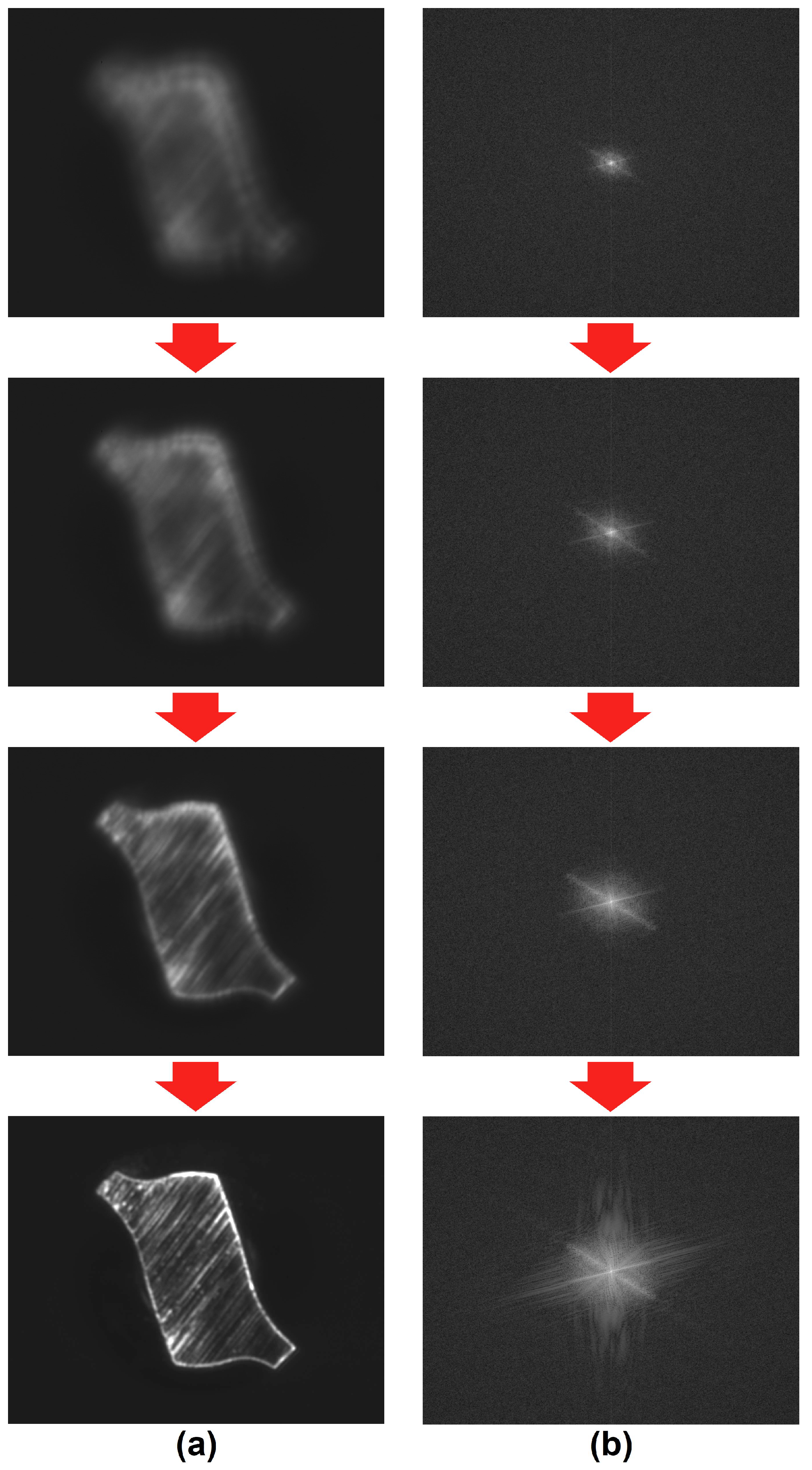
Figure 13.
Illustrative example of the variation curve of the relative focusing index Γ with respect to the Y-axial relative position.
Figure 13.
Illustrative example of the variation curve of the relative focusing index Γ with respect to the Y-axial relative position.
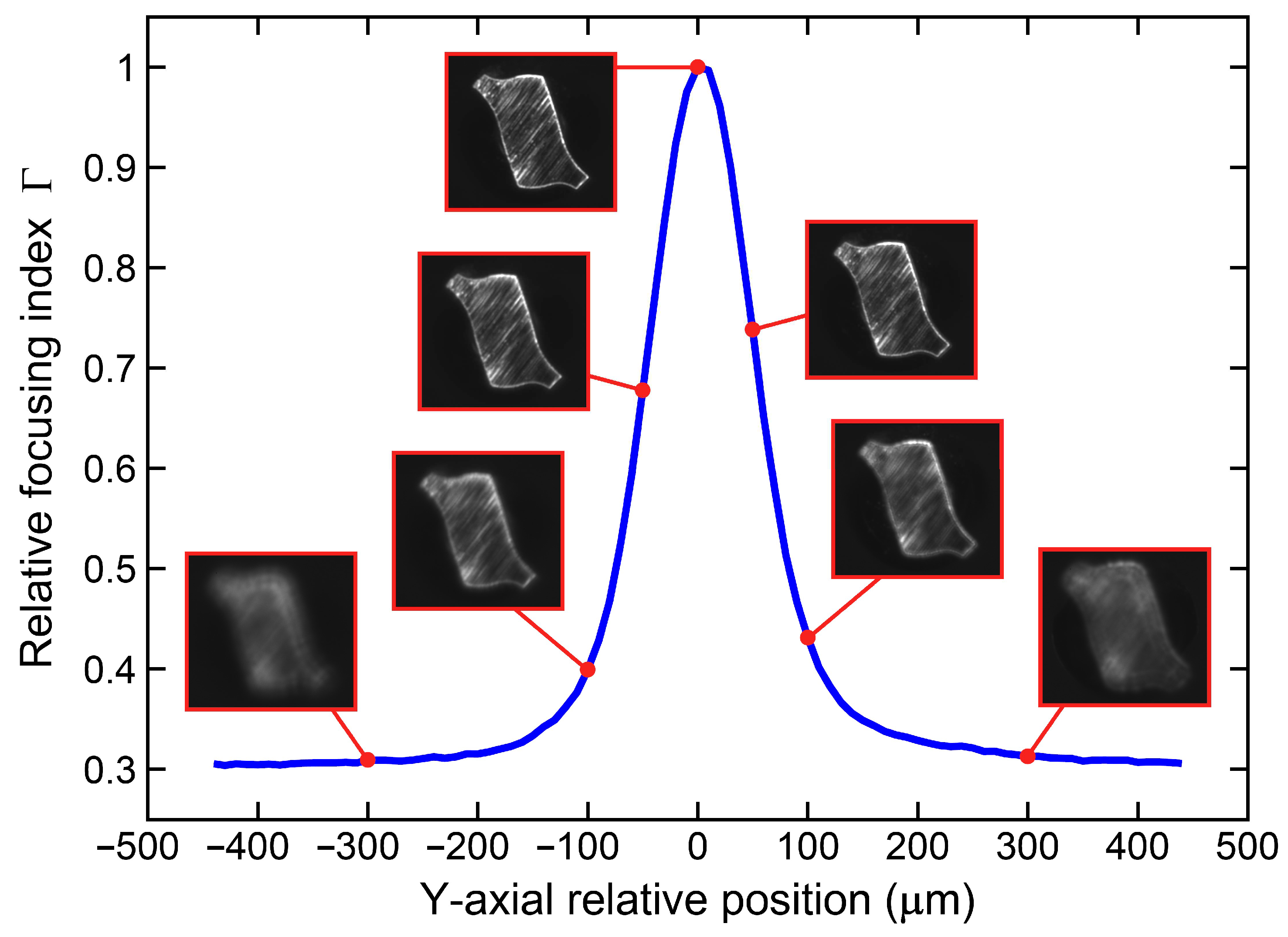
Figure 14.
Illustration of the sequential operations of the WTM sub-process.
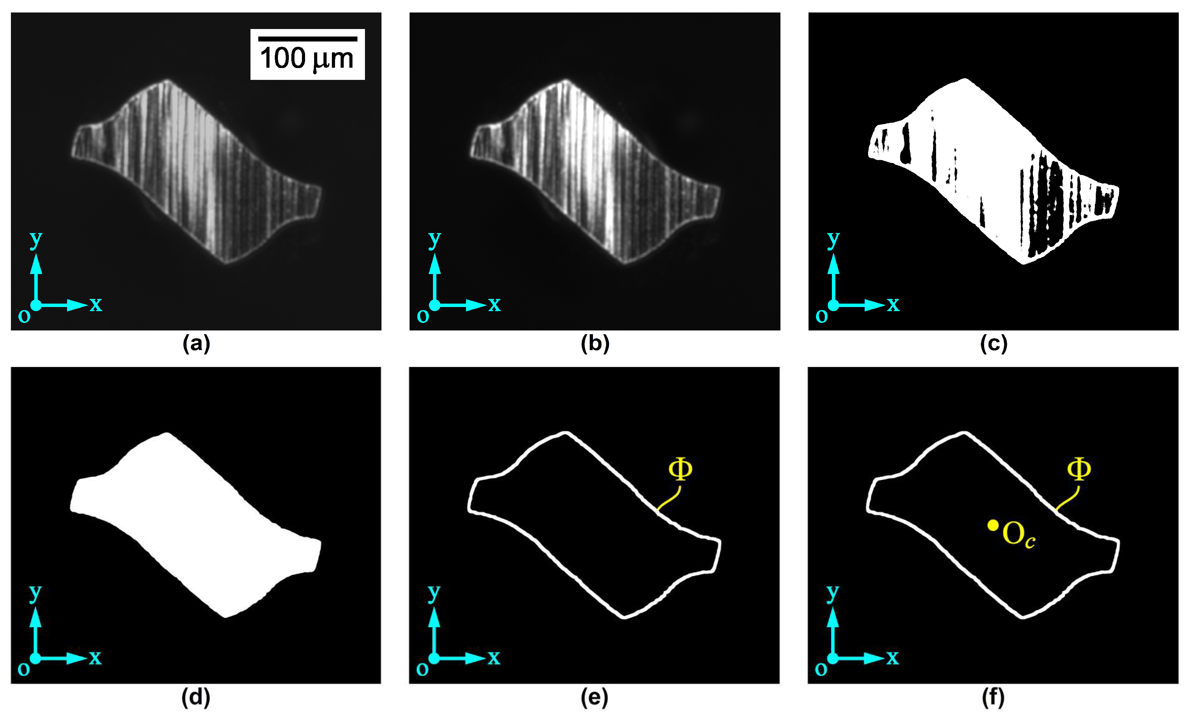
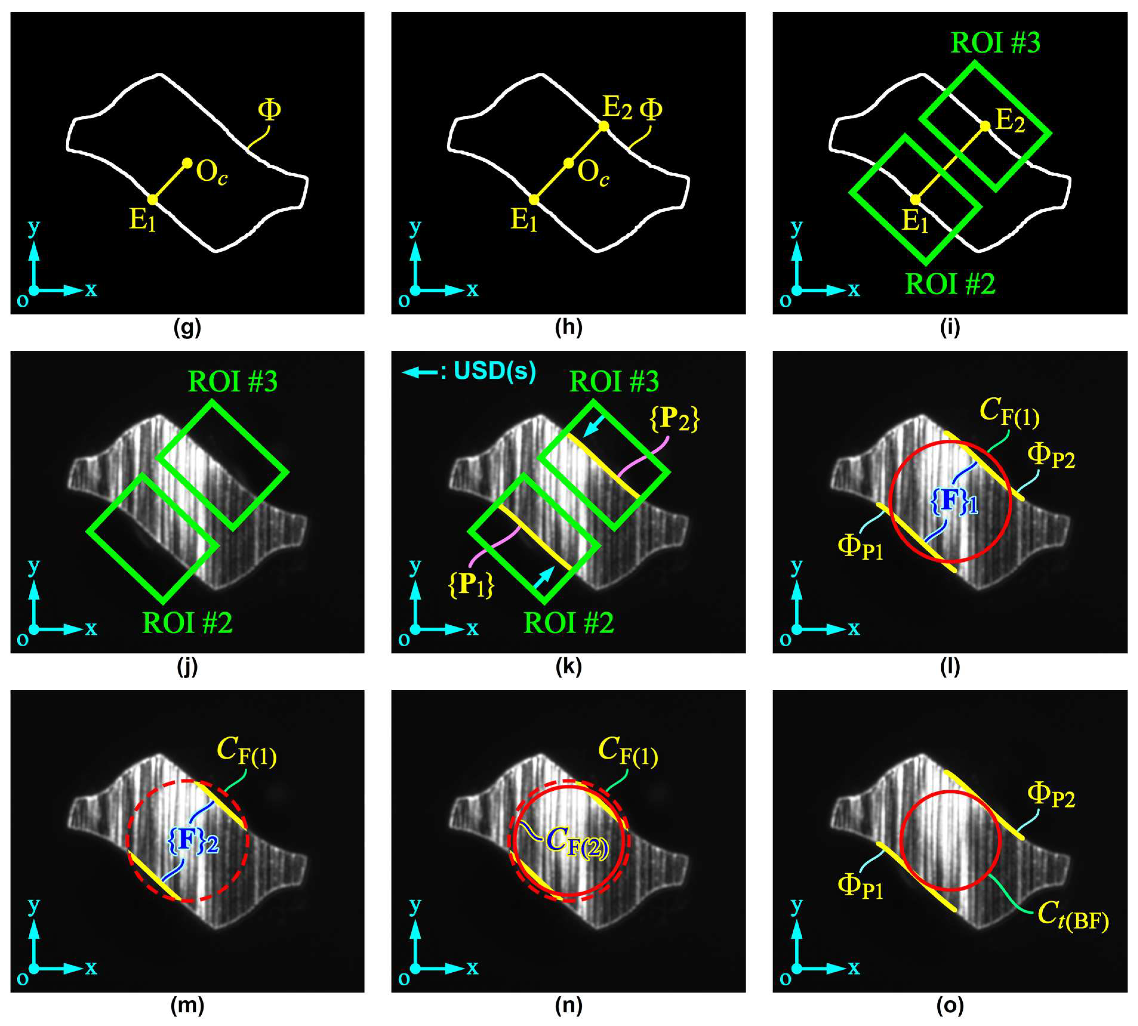
Figure 15.
Illustration of the sequential operations of the ODM sub-process.
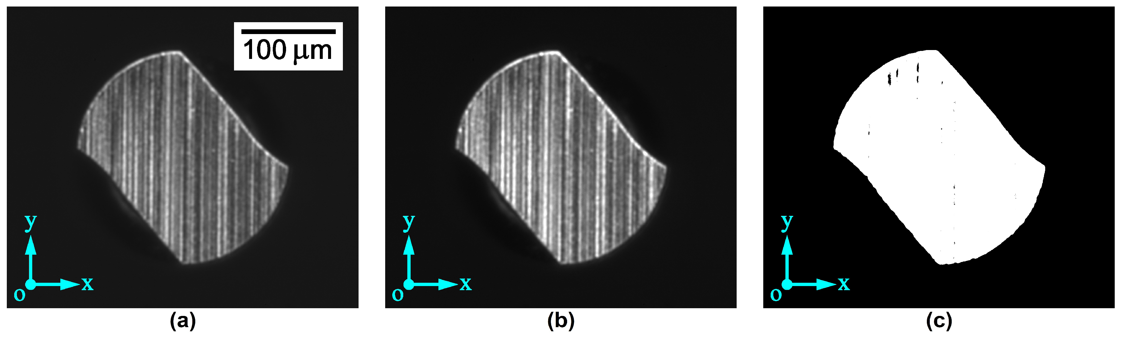
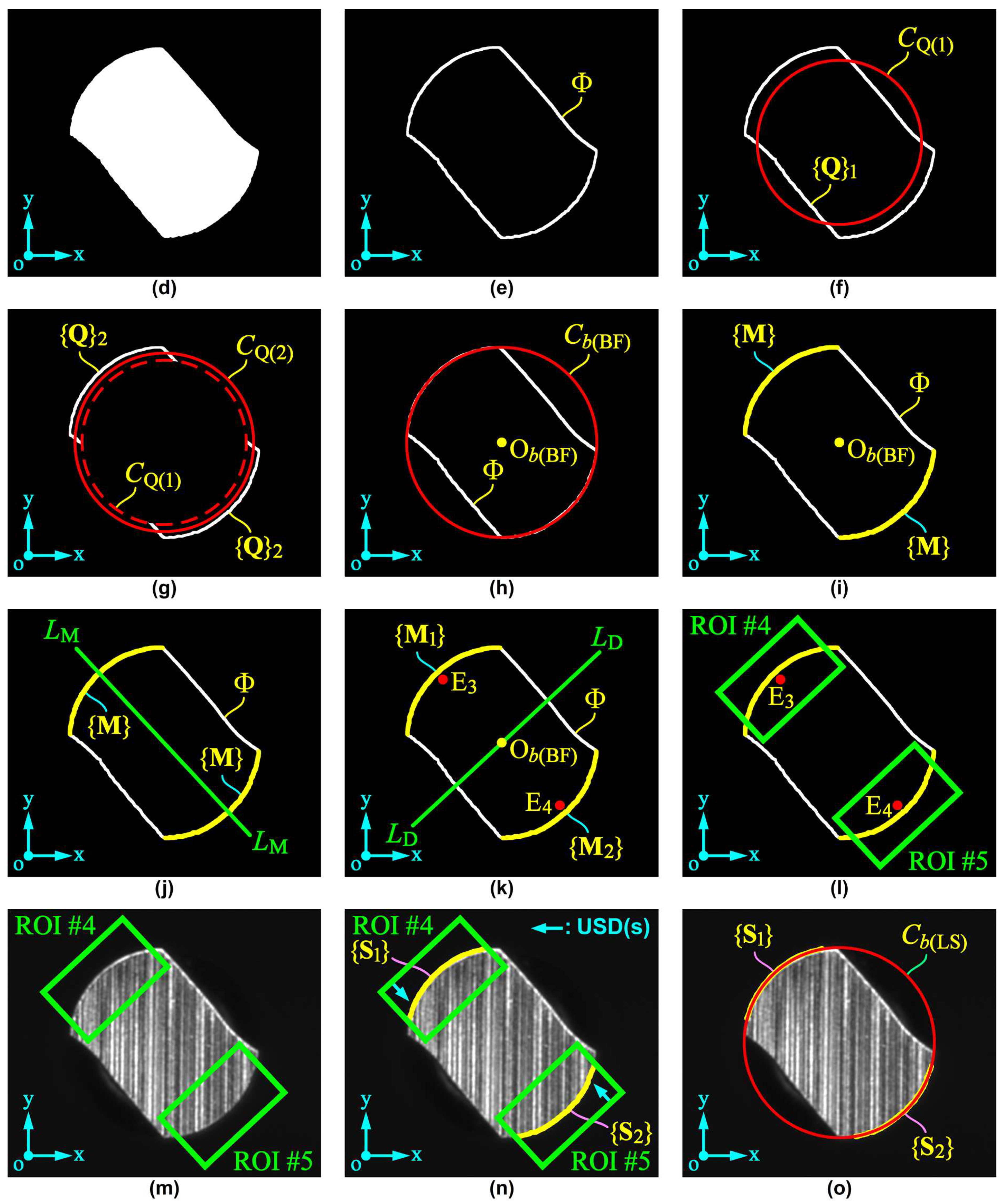
Figure 16.
Measuring the CSGPs of a microdrill sample by a measuring microscope.

Figure 17.
Measured values and fitted curves of the CSWTs of certain microdrill samples.
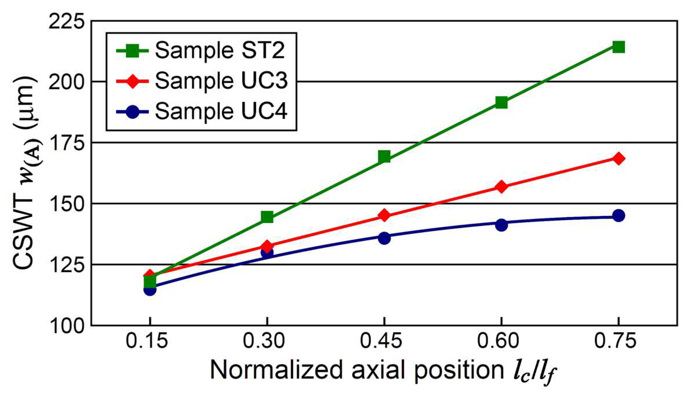

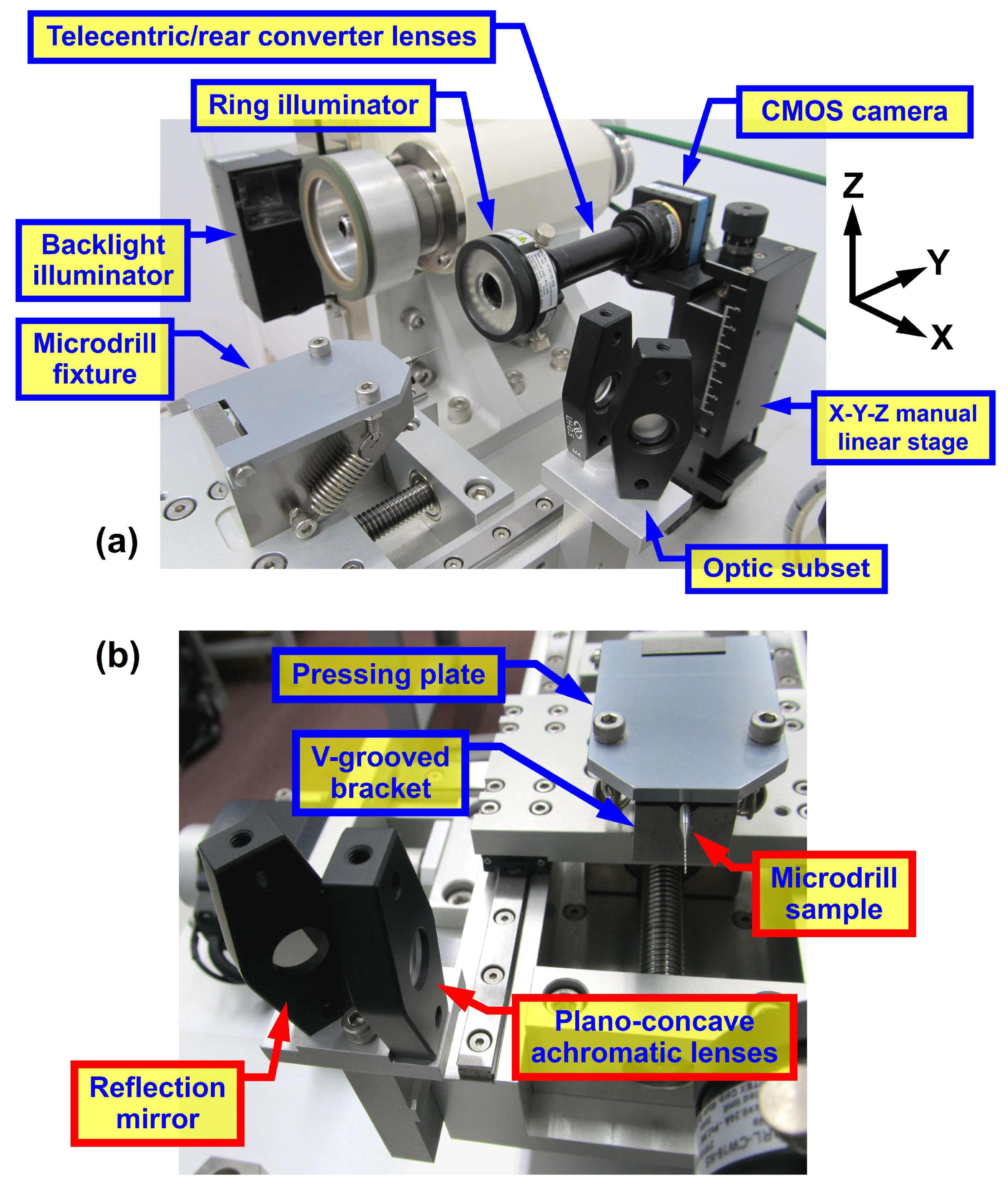
Table 1.
Statistical results for the measurements of sample ST1 (Dn = 0.30 mm and lf = 5.5 mm).
| Axial Position lc = 0.15lf | Axial Position lc = 0.45lf | |||||||||||
| CSGP Measured by the Developed System | CSGP Measured by Measuring Microscope | CSGP Measured by the Developed System | CSGP Measured by Measuring Microscope | |||||||||
| Statistical Term | w(A) (μm) | D(A) (μm) | ∆C(A) (μm) | w(M) (μm) | D(M) (μm) | ∆C(M) (μm) | w(A) (μm) | D(A) (μm) | ∆C(A) (μm) | w(M) (μm) | D(M) (μm) | ∆C(M) (μm) |
| Measured maximum | 119.17 | 295.31 | 1.94 | 119.07 | 295.93 | 18.12 | 169.56 | 292.32 | 2.23 | 170.10 | 292.87 | 19.10 |
| Measured minimum | 118.51 | 294.62 | 0.70 | 117.06 | 294.13 | 1.35 | 168.75 | 291.59 | 1.32 | 168.33 | 290.85 | 3.98 |
| Mean value μ | 118.86 | 294.89 | 1.13 | 118.21 | 295.09 | 9.11 | 169.11 | 291.94 | 1.92 | 169.29 | 291.70 | 9.57 |
| Standard deviation σ | 0.179 | 0.195 | 0.395 | 0.590 | 0.690 | 6.196 | 0.182 | 0.175 | 0.244 | 0.549 | 0.565 | 5.043 |
| Uncertainty ũ | 0.538 | 0.584 | 1.314 | 1.771 | 2.069 | 18.173 | 0.547 | 0.525 | 0.871 | 1.646 | 1.694 | 16.991 |
| Upper bound β(u) | 119.40 | 295.47 | 1.94 | 119.98 | 297.16 | 18.79 | 169.65 | 292.46 | 2.28 | 170.94 | 293.40 | 20.15 |
| Lower bound β(l) | 118.32 | 294.30 | 0.63 | 116.44 | 293.02 | 0.61 | 168.56 | 291.41 | 1.41 | 167.65 | 290.01 | 3.16 |
Table 2.
Statistical results for the measurements of sample UC1 (Dn = 0.25 mm and lf = 3.9 mm).
| Axial Position lc = 0.15lf | Axial Position lc = 0.45lf | |||||||||||
| CSGP Measured by the Developed System | CSGP Measured by Measuring Microscope | CSGP Measured by the Developed System | CSGP Measured by Measuring Microscope | |||||||||
| Statistical Term | w(A) (μm) | D(A) (μm) | ∆C(A) (μm) | w(M) (μm) | D(M) (μm) | ∆C(M) (μm) | w(A) (μm) | D(A) (μm) | ∆C(A) (μm) | w(M) (μm) | D(M) (μm) | ∆C(M) (μm) |
| Measured maximum | 120.61 | 222.97 | 1.72 | 121.91 | 223.36 | 17.86 | 150.29 | 225.14 | 1.85 | 150.44 | 225.88 | 17.16 |
| Measured minimum | 119.88 | 222.44 | 0.94 | 119.34 | 221.26 | 1.38 | 149.37 | 224.08 | 0.62 | 148.24 | 223.87 | 1.46 |
| Mean value μ | 120.12 | 222.67 | 1.37 | 120.24 | 222.58 | 8.32 | 149.86 | 224.52 | 1.33 | 149.01 | 224.62 | 7.84 |
| Standard deviation σ | 0.206 | 0.152 | 0.216 | 0.732 | 0.653 | 5.655 | 0.321 | 0.328 | 0.416 | 0.653 | 0.547 | 4.551 |
| Uncertainty ũ | 0.619 | 0.456 | 0.770 | 2.196 | 1.958 | 19.304 | 0.964 | 0.985 | 1.332 | 1.959 | 1.641 | 14.995 |
| Upper bound β(u) | 120.74 | 223.13 | 1.73 | 122.43 | 224.53 | 20.49 | 150.83 | 225.51 | 1.90 | 150.97 | 226.26 | 16.17 |
| Lower bound β(l) | 119.50 | 222.22 | 0.96 | 118.04 | 220.62 | 1.18 | 148.90 | 223.54 | 0.56 | 147.05 | 222.98 | 1.18 |
Table 3.
Statistical results for the measurements of sample UC2 (Dn = 0.20 mm and lf = 3.0 mm).
| Axial Position lc = 0.15lf | Axial Position lc = 0.45lf | |||||||||||
| CSGP Measured by the Developed System | CSGP Measured by Measuring Microscope | CSGP Measured by the Developed System | CSGP Measured by Measuring Microscope | |||||||||
| Statistical Term | w(A) (μm) | D(A) (μm) | ∆C(A) (μm) | w(M) (μm) | D(M) (μm) | ∆C(M) (μm) | w(A) (μm) | D(A) (μm) | ∆C(A) (μm) | w(M) (μm) | D(M) (μm) | ∆C(M) (μm) |
| Measured maximum | 126.35 | 201.85 | 3.32 | 126.64 | 202.71 | 18.74 | 141.93 | 187.22 | 2.66 | 141.94 | 187.83 | 18.64 |
| Measured minimum | 125.38 | 201.23 | 2.31 | 125.14 | 201.11 | 1.37 | 141.30 | 186.60 | 1.24 | 140.31 | 185.86 | 3.43 |
| Mean value μ | 125.74 | 201.46 | 2.69 | 126.02 | 201.88 | 6.91 | 141.68 | 186.93 | 1.63 | 141.16 | 186.66 | 10.25 |
| Standard deviation σ | 0.317 | 0.226 | 0.350 | 0.575 | 0.594 | 4.962 | 0.234 | 0.215 | 0.374 | 0.610 | 0.581 | 5.575 |
| Uncertainty ũ | 0.950 | 0.679 | 1.201 | 1.725 | 1.782 | 16.651 | 0.701 | 0.646 | 1.481 | 1.829 | 1.744 | 17.946 |
| Upper bound β(u) | 126.69 | 202.14 | 3.42 | 127.74 | 203.66 | 17.10 | 142.38 | 187.57 | 2.72 | 142.99 | 188.40 | 20.17 |
| Lower bound β(l) | 124.79 | 200.78 | 2.22 | 124.29 | 200.10 | 0.45 | 140.98 | 186.28 | 1.24 | 139.34 | 184.91 | 2.23 |
Table 4.
Statistical results for the measurements of sample ST2 (Dn = 0.30 mm and lf = 5.5 mm).
| Normalized Axial Position | CSGP Measured by the Developed System | CSGP Measured by Measuring Microscope | Absolute Difference | ||||
| lc/lf | w(A) (μm) a | D(A) (μm) | ∆C(A) (μm) | w(M) (μm) | D(M) (μm) | |w(A) − w(M)| (μm) | |D(A) − D(M)| (μm) |
| 0.15 | 117.97 | 294.78 | 1.82 | 117.23 | 295.85 | 0.74 | 1.07 |
| 0.30 | 144.53 | 293.36 | 3.37 | 145.46 | 294.95 | 0.93 | 1.59 |
| 0.45 | 169.38 | 291.33 | 1.43 | 170.60 | 290.55 | 1.22 | 0.78 |
| 0.60 | 191.54 | 291.40 | 2.22 | 191.17 | 293.14 | 0.37 | 1.74 |
| 0.75 | 214.24 | 289.95 | 0.80 | 213.79 | 288.60 | 0.45 | 1.35 |
a Fitted linear regression model: w(A) ≈ 159.700(lc/lf) + 95.666 μm (with a norm of residuals of 2.913 μm).
Table 5.
Statistical results for the measurements of sample UC3 (Dn = 0.25 mm and lf = 3.9 mm).
| Normalized Axial Position | CSGP Measured by the Developed System | CSGP Measured by Measuring Microscope | Absolute Difference | ||||
| lc/lf | w(A) (μm) a | D(A) (μm) | ∆C(A) (μm) | w(M) (μm) | D(M) (μm) | |w(A) − w(M)| (μm) | |D(A) − D(M)| (μm) |
| 0.15 | 120.37 | 223.85 | 2.46 | 119.55 | 222.73 | 0.82 | 1.12 |
| 0.30 | 132.45 | 221.72 | 2.22 | 130.96 | 221.37 | 1.49 | 0.35 |
| 0.45 | 145.28 | 223.50 | 1.91 | 146.18 | 224.39 | 0.90 | 0.89 |
| 0.60 | 156.95 | 223.88 | 2.04 | 158.78 | 223.14 | 1.83 | 0.74 |
| 0.75 | 168.49 | 224.67 | 1.31 | 169.16 | 226.08 | 0.67 | 1.41 |
a Fitted linear regression model: w(A) ≈ 80.490(lc/lf) + 108.490 μm (with a norm of residuals of 0.749 μm).
Table 6.
Statistical results for the measurements of sample UC4 (Dn = 0.20 mm and lf = 3.0 mm).
| Normalized Axial Position | CSGP Measured by the Developed System | CSGP Measured by Measuring Microscope | Absolute Difference | ||||
| lc/lf | w(A) (μm) a | D(A) (μm) | ∆C(A) (μm) | w(M) (μm) | D(M) (μm) | |w(A) − w(M)| (μm) | |D(A) − D(M)| (μm) |
| 0.15 | 114.77 | 207.74 | 2.76 | 115.40 | 208.94 | 0.63 | 1.20 |
| 0.30 | 129.94 | 188.23 | 1.79 | 130.54 | 186.91 | 0.60 | 1.32 |
| 0.45 | 135.78 | 187.03 | 2.03 | 134.37 | 186.39 | 1.41 | 0.64 |
| 0.60 | 141.16 | 186.81 | 1.85 | 142.25 | 187.99 | 1.09 | 1.18 |
| 0.75 | 145.11 | 185.64 | 1.31 | 144.08 | 184.23 | 1.03 | 1.41 |
a Fitted second-order regression model: w(A) ≈ −72.724(lc/lf)2 + 113.384(lc/lf) + 100.330 μm (with a norm of residuals of 2.761 μm).
Disclaimer/Publisher’s Note: The statements, opinions and data contained in all publications are solely those of the individual author(s) and contributor(s) and not of MDPI and/or the editor(s). MDPI and/or the editor(s) disclaim responsibility for any injury to people or property resulting from any ideas, methods, instructions or products referred to in the content. |
© 2023 by the authors. Licensee MDPI, Basel, Switzerland. This article is an open access article distributed under the terms and conditions of the Creative Commons Attribution (CC BY) license (https://creativecommons.org/licenses/by/4.0/).
Share and Cite
MDPI and ACS Style
Chang, W.-T.; Lu, Y.-Y. An Improved Automation System for Destructive and Visual Measurements of Cross-Sectional Geometric Parameters of Microdrills. Machines 2023, 11, 581. https://doi.org/10.3390/machines11060581
AMA Style
Chang W-T, Lu Y-Y. An Improved Automation System for Destructive and Visual Measurements of Cross-Sectional Geometric Parameters of Microdrills. Machines. 2023; 11(6):581. https://doi.org/10.3390/machines11060581
Chicago/Turabian StyleChang, Wen-Tung, and Yu-Yun Lu. 2023. "An Improved Automation System for Destructive and Visual Measurements of Cross-Sectional Geometric Parameters of Microdrills" Machines 11, no. 6: 581. https://doi.org/10.3390/machines11060581
Note that from the first issue of 2016, this journal uses article numbers instead of page numbers. See further details here.