Decentralized Adaptive Quantized Dynamic Surface Control for a Class of Flexible Hypersonic Flight Vehicles with Input Quantization

Abstract

A control strategy for a certain class of hypersonic flight aircraft dynamic models with unknown parameters is proposed in this article. The strategy is adaptive dynamic surface input quantization control. To address the issues in conventional inversion control, a first-order low-pass filter and an adaptive parameter minimum learning law are introduced in the control system design process. This method has the following features: (1) it solves the problem of repeated differentiation of the virtual control law in the conventional back-stepping method, greatly simplifying the control law structure; (2) by using the norm of the neural network weight vector as the adaptive adjustment parameter instead of updating each element online, the number of adaptive adjustment parameters is significantly reduced, improving the execution efficiency of the controller; (3) the introduced hysteresis quantizer overcomes the disadvantage of the quantization accuracy deterioration when the input value is too low in the logarithm quantizer, improving the accuracy of the quantizer. Stability analysis has shown that all signals in the closed-loop system are semi-globally uniformly bounded, and simulation results have verified the effectiveness of the proposed adaptive quantized control scheme.

1. Introduction

As an effective means of transportation for human entry into space, hypersonic flight aircraft (HFA) have a wide range of potential applications in future aerospace systems and have been the focus of scholars around the world over the past fifty years [1,2,3,4]. At the same time, as strategic aircraft, Hypersonic Flight Aircraft offer advantages such as quick response and high-precision strike capabilities. This makes the design and development of HFA automatic control systems an important scientific and technological field, and a crucial strategic demand for many countries. With the advancement of technologies such as computers, sensors, and actuators, the implementation of these control systems has become possible. Their purpose is to enhance aircraft intelligence and adaptability, ultimately improving overall performance and reliability. However, unlike ordinary subsonic or supersonic aircraft, supersonic aircraft are a new type of aircraft that operate in a large airspace, at ultra-high speeds (exceeding Mach 5), over long distances, and with high precision. Its overall layout adopts a special design structure of integrated air frame and engine, which makes each subsystem strongly coupled and strongly nonlinear. At the same time, the complex flight environment and parameter uncertainties of the model structure pose great challenges to the stability performance and control system design of the aircraft. Therefore, it is particularly important to study adaptive controller design methods that can overcome the system uncertainty [5,6,7,8,9].

Efficiently dealing with uncertainty in hypersonic flight systems is a hot topic in the field of hypersonic flight aircraft control. A s early as 2012, Ref. [10] designed an adaptive robust linear quadratic regulator (LQR) by linearizing the dynamic model to solve the problem of parameter uncertainty in the system. However, linearization has limitations when dealing with the strong nonlinearity and coupling characteristics of hypersonic flight dynamics. With the continuous development of control technology, advanced intelligent control methods such as intelligent learning strategies, including neural networks and fuzzy systems, have been widely applied in the design process of hypersonic flight control systems, as shown in references [6,11].

Another approach to effectively deal with the uncertainties in aerodynamic parameters or unknown nonlinearities during the flight of hypersonic flight aircraft (HFA) is to estimate the HFA model uncertainty online and apply function learning and feed forward compensation. In addition, to efficiently handle the wind effects and unknown external disturbances during the flight of hypersonic flight vehicles, disturbance observers have been introduced in literature [12,13,14], achieving good control performance. In [15], the author designed an H-infinity feedback controller for the linearized model of the oxygenator through the solution of the Riccati equation at each iteration of the control strategy. A positive definite weight matrix was introduced for the calculation of the feedback control gain, achieving the H-infinity tracking performance standard of the control system, and a hybrid control scheme has been proposed for combustion process in heating furnace of compact strip production based on condition identification. The experimental results in a steel plant showed that the proposed control scheme significantly improved the precision of furnace temperature control and reduced energy consumption, achieving good control effects [16].

Back stepping control is an efficient control strategy for nonlinear and uncertain systems that designs controllers based on the physical model of the system and the inverse model of the controller. Back stepping control method has strong adaptability and robustness, which can effectively solve the problems such as uncertainty and external disturbances in the system [17,18,19]. However, during the design process, this method requires repeated differentiation of the virtual control law, which may lead to the “differential explosion” phenomenon, resulting in highly complex controllers, especially when the system order increases, such as in 3rd order and above. Therefore, the characteristics of the system and the applicability of inverted control must be fully considered in practical applications. To overcome the limitations of back stepping method, the dynamic surface control (DSC) method has been proposed [20,21,22,23,24,25]. This method introduces a first-order low-pass filter in the each design process, which separates the coupling between the previous and the next steps, solves the problem of repeated differentiation of the virtual control law, and overcomes the differential explosion phenomenon. The DSC method has been widely used, including in the control of hypersonic aircraft. To achieve stability and robustness of hypersonic flight aircraft and address issues such as nonlinearity, uncertainty, and external disturbances, controllers have been designed using dynamic surface control method in [12,13], which respectively consider problems such as actuator faults, unknown nonlinearities, and time delays while ensuring system stability and performance indicators. Qiao considers issues such as input saturation and external disturbances and also designs controllers using dynamic surface control method to achieve system stability and performance requirements [14].

Currently, digital computer controllers play an important role in control systems, with control signals often generated by computers and transmitted in communication channels. To improve communication efficiency, control signals need to be quantized before entering the communication channel [26,27,28,29,30]. Therefore, to improve control accuracy, the quantization effect of quantizers should be considered in controller design to eliminate the impact of quantization errors on control performance [25,31,32,33]. In [28], a robust stabilization method for uncertain linear systems is introduced, which includes an input quantizer as part of the controller. The author uses a method based on H∞ control theory and quadratic stability to design the robust controller, and considers the effect of the input quantizer. In [29], a control method for linear parameter-varying systems based on quantized state feedback is discussed. The author designed a stabilizing controller using Lyapunov functions and incorporated the influence of the quantizer into the system model. Additionally, the author also discussed the impact of the input quantizer on system performance. In [34], a fuzzy adaptive tracking control algorithm for high-speed supersonic aircraft with input quantization and faults was proposed, and an error transformation function was established to ensure the tracking error of the system. In [35], an backstepping control method was used in conjunction with an interval type-2 fuzzy neural network (IT2FNN) to design a quantization mechanism tracking control scheme for a class of HFA with prescribed performance. The uncertainty in the system was approximated using a type-2 fuzzy neural network, and a new control law was designed for the quantization mechanism.

In addition, in adaptive control schemes, neural networks [5,17,18,36] or fuzzy systems [19,29] are often used to compensate for uncertainty and unknown dynamics in the system online. In [37], a novel reference tracking control method has been proposed for servo system, and the experimental results show that the Grey Wolf Optimizer method can solve the main shortcomings of the Gradient Descent scheme in Reinforcement Learning-based control problems. However, the online adjustment of parameters often increases as the input-output dimension and number of nodes of the neural network or fuzzy system increase, leading to excessive computational requirements and decreased control system efficiency. Therefore, to address the issue of excessive online adaptive parameter adjustment in adaptive control schemes, a minimal learning method has been proposed [38,39,40,41,42], here, by estimation of the weight vector norm of neural networks, each step of the controller design process can update only one parameter online, greatly reducing the system’s computational requirements and improving the control system’s execution efficiency.

Inspired by the literature mentioned above, this paper proposes a quantized input control scheme based on the minimum learning method for a class of hypersonic vehicles. In contrast to previous literature, dynamic surface control is introduced to address the problem of differential explosion in the backstepping control scheme, simplify the final controller structure, and reduce the complexity of controller design. The hysteresis quantizer is introduced to address the disadvantage of reduced quantization accuracy in the quantizer when the input value is too low, thereby improving the accuracy of the quantizer. By introducing the minimum learning method, the problem of too many online updated parameters in conventional adaptive control is addressed, reducing the system’s computational complexity and improving control efficiency.

The remaining parts of this paper are structured as follows. In Section 2, the background of the problem, the dynamic model of hypersonic aircraft and its general form, as well as the quantizer and neural network are introduced. Section 3 describes the process of controller design and the stability analysis of the system. In Section 4, a set of experimental results and their corresponding design parameters are presented. Finally, the paper is concluded in Section 5.

2. HFA Mathematical Model and Preliminaries

2.1. HFA Dynamic Model

The aerodynamics of hypersonic vehicles exhibit strong coupling and high nonlinearity. A ccording to the literature [43,44,45], the mathematical model of the HFA can be described as follows:

$$\begin{array}{cc}\hfill \dot{V}& =\frac{Tcos\alpha -D}{m}-gsin\gamma ,\hfill \\ \hfill \dot{h}& =Vsin\gamma ,\hfill \\ \hfill \dot{\gamma }& =\frac{L+Tsin\alpha }{mV}-\frac{gcos\left(\gamma \right)}{V},\hfill \\ \hfill \dot{\alpha }& =q-\dot{\gamma },\hfill \\ \hfill \dot{q}& =\frac{M_{yy}}{I_{yy}}+\frac{{\tilde{\psi }}_1{\ddot{\eta }}_1}{I_{yy}}+\frac{{\tilde{\psi }}_2{\ddot{\eta }}_2}{I_{yy}},\hfill \end{array}$$

(1)

with the

$${\ddot{\eta }}_i=-2{\iota }_i{\zeta }_i{\dot{\eta }}_i-{\zeta }_i^2{\eta }_i+N_i+{\tilde{\psi }}_i\dot{q}$$

(2)

here, the velocity is denoted by V, the flight path angle by $\gamma$, the altitude by h, the attack angle by $\alpha$, the pitch rate by q. A nd ${\eta }_i,(i=1,2)$ are the flexible states of HFA. The thrust, drag, lift-force, and pitching moment are represented by $T\left(V,\beta \right)$, $D\left(V,\alpha \right)$, $L\left(V,\alpha \right)$ and $M_{yy}\left(V,\alpha ,q,{\delta }_E\right)$, respectively, and can be expressed as:

$$\begin{array}{cc}\hfill T& =C_T^{{\alpha }^3}{\alpha }^3+C_T^{{\alpha }^2}{\alpha }^2+{C_T}^{\alpha }\alpha +C_T^0,\hfill \\ \hfill D& =\overline{q}S{C}_D\left(\alpha ,{\delta }_e\right),\hfill \\ \hfill L& =\overline{q}S{C}_L\left(\alpha ,{\delta }_e\right),\hfill \\ \hfill M_{yy}& =z_{T}T+\overline{q}S\overline{c}[C_{M,\alpha }\left(\alpha \right)+C_{M,{\delta }_e}\left({\delta }_e\right)],\hfill \end{array}$$

with $C_L=C_L^{\alpha }\alpha +C_L^0,$ $C_D=C_D^{{\alpha }^2}{\alpha }^2+C_D^{\alpha }\alpha +C_D^0,$ $C_{M,\alpha }\left(\alpha \right)=C_{M,\alpha }^{{\alpha }^2}{\alpha }^2+C_{M,\alpha }^{\alpha }\alpha +C_{M,\alpha }^0,$ $C_T^{{\alpha }^3}={\beta }_1\Phi +{\beta }_2,$ $C_T^{{\alpha }^2}={\beta }_3\Phi +{\beta }_4,$ $C_T^{\alpha }={\beta }_5\Phi +{\beta }_6,$ $C_T^0={\beta }_7\Phi +{\beta }_8,$ $\overline{q}=\rho V^2/2,$ and $\rho ={\rho }_{0}exp\left(-\left(h-h_0\right)/h_s\right),$ where ${\delta }_e$, $\Phi$ are denote the elevator deflection and throttle setting, respectively. Letting $\theta$ denote the pitch angle, we have $\theta =\alpha +\gamma$. Then, we define state variables as $x={[x_V,x_h,x_{\gamma },x_{\theta },x_q]}^T$, with $x_V=V$, $x_h=h$, $x_{\gamma }=\gamma$, $x_{\theta }=\theta$ and $x_q=q$. $u={[{\delta }_e,\Phi ]}^T$ is the control input. Note that during trimmed cruise condition, the flight path angle $\gamma$ is typically very small, which justifies the approximation $sin\left(\gamma \right)\approx \gamma$. Therefore Equation (1) can be rewritten as

$$\begin{array}{cc}\hfill \dot{x}& =f\left(x\right)+g\left(x\right)u,\hfill \\ \hfill y& =[x_V,x_h],\hfill \end{array}$$

(3)

where $f\left(x\right)={[f_V\left(x\right),f_h\left(x\right),f_{\gamma }\left(x\right),f_{\theta }\left(x\right),f_q\left(x\right)]}^T$, $g\left(x\right)=[g_V\left(x\right),g_h\left(x\right),g_{\gamma }\left(x\right),g_{\theta }\left(x\right),g_q{\left(x\right)]}^T$, $f_V\left(x\right)=\left({\beta }_a{\phi }_{0}cos\alpha -D\right)/m-gsin\gamma$, $f_h\left(x\right)=0$, $f_{\gamma }=\overline{q}S\left(C_L^0-C_L^{\alpha }{x}_h\right)/mV+Tsin\alpha /mV-gcos{x}_h/V$, $f_{\theta }\left(x\right)=0$, $f_q=\left(z_{T}T+\overline{q}S\overline{c}{C}_{M,\alpha }\left(\alpha \right)\right)/I_{yy}$, $g_V\left(x\right)={\beta }_b{\phi }_{0}cos\alpha /m$, $g_h\left(x\right)=V$, $g_{\gamma }\left(x\right)=\overline{q}S{C}_L^{\alpha }/mV$, $g_{\theta }\left(x\right)=1$, $g_q\left(x\right)=\overline{q}S\overline{c}{c}_e/I_{yy}$, ${\beta }_a=\left[{\beta }_2,{\beta }_4,{\beta }_6,{\beta }_8\right]$, ${\beta }_b=\left[{\beta }_1,{\beta }_3,{\beta }_5,{\beta }_7\right]$, and ${\phi }_0={\left[{\alpha }^3,{\alpha }^2,\alpha ,1\right]}^T$. The inertial and aerodynamic parameters’ values being uncertain implies that the functions $f_i\left(x\right)$ and $g_i\left(x\right)$, $i=V,h,\gamma ,\theta ,q$, are unknown. Additionally, as mentioned in [44,45], the model of the HFA indicates that $g_V\left(x\right)$, $g_h\left(x\right)$ and $g_{\gamma }\left(x\right)$ are strictly positive, while $g_q\left(x\right)$ is strictly negative due to $c_e$ being negative.

2.2. RBF Neural Networks

Mathematically speaking, the utilization of Radial Basis Function Neural Networks (RBFNNs) was employed in this study to estimate continuous unknown functions within a designated compact set. A n RBFNN, as expressed in [46,47], can take the following form:

$$F\left(\xi \right)={\vartheta }^T\psi \left(\xi \right),$$

(4)

where $F\in \mathbb{R}$ and $\xi \in {\mathbb{R}}^n$ represent the network output and input, respectively $\vartheta \in {\mathbb{R}}^n$ is the weight vector, and $\psi \left(\xi \right)={\left[{\psi }_1\left(\xi \right),\cdots ,{\psi }_N\left(\xi \right)\right]}^T$ is the basis function vector. typically, the basis function vector ${\psi }_i\left(\xi \right)$ are selected as Gaussion functions:

$${\psi }_i\left(\xi \right)=\frac{1}{\sqrt{2\pi }b}exp\left(-\frac{{∥\xi -{\xi }_i∥}^2}{2b^2}\right),b>0,i=0,\dots ,N,$$

(5)

the constants ${\xi }_i\in {\mathbb{R}}^n$ and $b\in \mathbb{R}$ are known as the center and width of the basis function, respectively.

Lemma 1.

Ref. [47] for any continuous function $F\left(\xi \right):{\Omega }_{\xi }\to \mathbb{R}$, where ${\Omega }_{\xi }\subset {\mathbb{R}}^n$ is a compact set, and any constant $ϵ>0,$ it is possible to appropriately select b and ${\xi }_i,i=1,\dots ,N,$ for some sufficiently large integer N, such that there exists an RBF NN ${\vartheta }^{\ast T}\psi \left(\xi \right)$ satisfying the equation

$$F\left(\xi \right)={\vartheta }^{\ast T}\psi \left(\xi \right)+\Delta \left(\xi \right),|\Delta \left(\xi \right)|\le ϵ,\forall \xi \in {\Omega }_{\xi },$$

(6)

here ${\vartheta }^{*}$ represents the optimal weight vector defined as

$${\vartheta }^{*}=arg\underset{W\in {\mathbb{R}}^n}{min}\left\{\underset{\xi \in {\Omega }_{\xi }}{sup}\left|\Psi \left(\xi \right)-{\vartheta }^T\psi \left(\xi \right)\right|\right\},$$

(7)

while $\Delta \left(\xi \right)$ represents the approximation error.

Remark 1.

In the design of adaptive control systems, RBF neural networks can effectively improve the performance of the controller when the system has significant uncertainty. In this paper, the RBF neural network is introduced to estimate the unknown terms in the FLA system online, and the adaptive laws can be derived using the Lyapunov method. The stability and convergence of the entire closed-loop system are ensured by adjusting the adaptive weights. Currently, many achievements have been published about using RBF neural networks to design adaptive controllers for nonlinear systems [48,49].

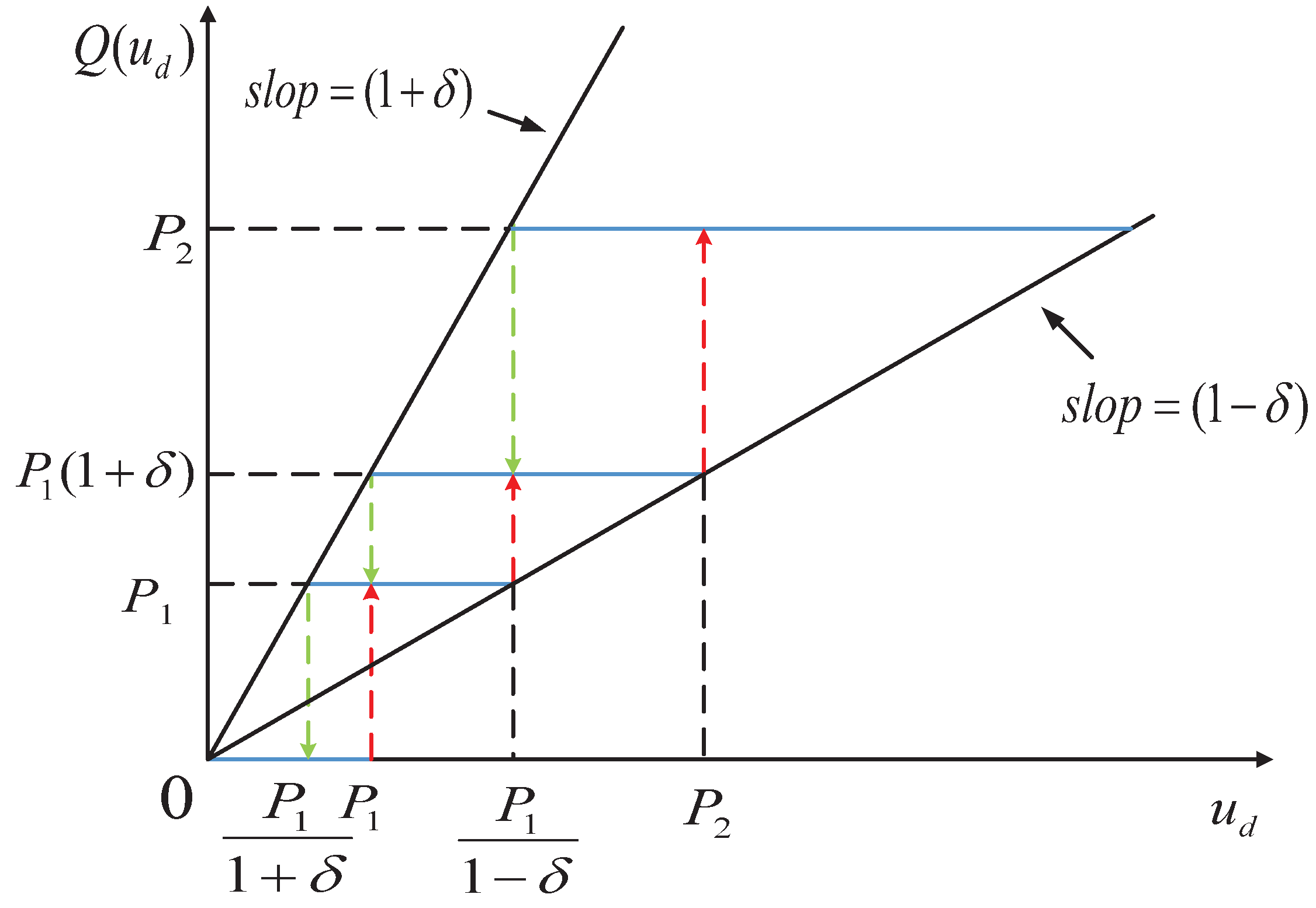
2.3. Quantizer with Hysteresis Characteristic

This paper achieves the computer control of FLA by introducing a hysteresis quantizer illustrated in Figure 1.

$$Q\left(u_i\right)=\left\{\begin{array}{c}{p}_{i,j},\mathrm{if}\frac{p_{i,j}}{1+{\delta }_i}<u_i\le p_{i,j},\\ Q^{-}\ge p_{i,j}\mathrm{or}{Q}^{-}\le p_{i,j}\\ p_{i,j}\le u_i<\frac{p_{i,j}}{1-{\delta }_i},\\ \left(1+{\sigma }_i\right)p_{i,j},\mathrm{if}{p}_{i,j}<u_i\le \frac{p_{i,j}}{1-{\delta }_i},\\ Q^{-}\ge \left(1+{\sigma }_i\right)p_{i,j},\\ \mathrm{or}\frac{p_{i,j}}{1-{\delta }_i}\le u_i<p_{i,j+1},\\ Q^{-}\le \left(1+{\sigma }_i\right)p_{i,j},\\ 0,\mathrm{if}0\le u_i\le \frac{p_{i,1}}{1+{\delta }_i}\\ \mathrm{or}\frac{p_{i,1}}{1+{\delta }_i}<u_i<p_{i,1},\\ Q^{-}=0,\\ -Q\left(-u_i\right),\mathrm{if}{u}_i<0,\end{array}\right.$$

(8)

Here, ${\delta }_i\left(t\right)=\frac{1-{ϵ}_i\left(t\right)}{1+{ϵ}_i\left(t\right)}$ and $p_{i,j}\left(t\right)=a_i\left(t\right){ϵ}_i^{1-j}\left(t\right)$, where $0<{ϵ}_i\left(t\right)<1$, $a_i\left(t\right)>0$ and $j=1,2,3\dots$ The parameter $a_i\left(t\right)$ determines the size of the dead-zone for $Q\left(u_i\right)$, while ${ϵ}_i\left(t\right)$ represents the density of the quantized signal. $Q^{-}$ represents the latest value of $Q\left(u_i\right)$. The maximum and minimum values of $a_i\left(t\right)$, ${ϵ}_i\left(t\right)$ are defined as ${\overline{a}}_i$, ${\underline{a}}_i$, ${\overline{ϵ}}_i,{\underline{ϵ}}_i$, respectively. For the quantized control signal, it is defined as:

$$l_{i1}=\left\{\begin{array}{c}\begin{array}{cc}\frac{Q\left(u_i\right)}{u_i}\hfill & \hfill ,\mathrm{if}|u_i|\ge a_i\left(t\right),\\ 1\hfill & \hfill ,\mathrm{if}|u_i|\le a_i\left(t\right),\end{array}\hfill \end{array}\right.$$

(9)

$$l_{i2}=\left\{\begin{array}{c}\begin{array}{cc}0\hfill & \hfill ,\mathrm{if}|u_i|\ge a_i\left(t\right),\\ Q\left(u_i\right)-u_i\hfill & \hfill ,\mathrm{if}|u_i|\le a_i\left(t\right).\end{array}\hfill \end{array}\right.$$

(10)

Then, we have

$$Q\left(u_i\right)=l_{i1}\left(t\right)u_i+l_{i2}\left(t\right).$$

(11)

From Figure 1, it can be obtained that

$$\begin{array}{c}\hfill 1-{\delta }_i\left(t\right)\le \frac{Q\left(u_i\right)}{u_i}\le 1+{\delta }_i\left(t\right),\mathrm{if}\left|u_i\right|\ge a_i\left(t\right),\\ \hfill |Q\left(u_i\right)-u_i|<a_i\left(t\right),\mathrm{if}\left|u_i\right|\le a_i\left(t\right),\end{array}$$

(12)

where

$$\begin{array}{c}\hfill l_{i1}\left(t\right)\ge {\lambda }_i,l_{i2}\left(t\right)\le {\overline{a}}_i,\forall t\ge 0\end{array}$$

(13)

with ${\lambda }_i>0$, such that ${\lambda }_i=\frac{2{ϵ}_{imin}}{1+{ϵ}_{imin}}$.

Remark 2.

Unlike the logarithmic quantizer, the introduced hysteresis quantizer in this article will stay a certain time interval during the transition between two different input values [50,51], and increases the quantization levels to overcome the vibration phenomenon that occurs in the logarithmic quantizer. The hysteresis quantizer can also adaptively adjust the quantization interval based on the amplitude of the control signals, compared to the logarithmic quantizer [52], significantly reducing the number of transitions and enhancing the ability to overcome chattering. It overcomes the problem of decreased quantization accuracy when the input value is too low in a quantizer, thus improving the accuracy of the quantizer.

3. Quantized Controller Design and Stability Analysis

Based on the parameterized Equation (1) of the HFA described in Section 3.1, the HFA control system is divided into two parts: velocity subsystem controller design and altitude subsystem controller design. Firstly, an adaptive quantized controller is designed for the velocity subsystem.

3.1. Velocity Subsystem Control Design

The velocity subsystem with input quantizer can be formulated as follows

$$\begin{array}{cc}\hfill {\dot{x}}_V& =f_V+g_{V}Q\left(\Phi \right),\hfill \\ \hfill y_1& =x_V=V,\hfill \end{array}$$

(14)

where $f_V$ and $g_V$ are supposed to be smooth functions with unknown parameters. $Q\left(\Phi \right)$ denotes the control input signal of velocity subsystem with hypersis quantizer. Then the tracking error of velocity is defined as

$$S_V=x_V-x_{Vd},$$

(15)

here $x_{Vd}$ is the velocity reference signal, then the time derivative of $S_V$ is

$$\begin{array}{cc}\hfill {\dot{S}}_V& ={\dot{x}}_V-{\dot{x}}_{Vd}\hfill \\ \hfill & =f_V\left({\overline{x}}_V\right)+g_{V}Q\left(\Phi \right)-{\dot{x}}_{Vd}\hfill \end{array}$$

(16)

To obtain the specific expression of $Q\left(\Phi \right)$, according to Equations (9)–(11), we define here

$${\iota }_{V1}\left(t\right)=\left\{\begin{array}{c}\frac{Q\left(\Phi \right)}{\Phi },\mathrm{if}\left|\Phi \right|\ge a_V\left(t\right)\\ 1,\mathrm{if}\left|\Phi \right|<a_V\left(t\right)\end{array}\right.$$

(17)

$${\iota }_{V2}\left(t\right)=\left\{\begin{array}{c}0,\mathrm{if}\left|\Phi \right|\ge a_V\left(t\right)\\ Q\left(\Phi \right)-\Phi ,\mathrm{if}\left|\Phi \right|<a_V\left(t\right)\end{array}\right.$$

(18)

Then the control signal can be obtain as

$$Q\left(\Phi \right)={\iota }_{V1}\left(t\right)\Phi +{\iota }_{V2}\left(t\right)$$

(19)

substituting (19) into (16) leads to

$${\dot{S}}_V=f_V\left({\overline{x}}_V\right)+g_V{\iota }_{V1}\left(t\right)\Phi +g_V{\iota }_{V2}\left(t\right)-{\dot{x}}_{Vd}$$

(20)

Equation (20) can be rewritten as

$${\dot{S}}_V=g_V(\frac{1}{g_V}{f}_V\left({\overline{x}}_V\right)-\frac{1}{g_V}{\dot{x}}_{Vd}+\frac{1}{2}{S}_V)+g_V({\iota }_{V1}\left(t\right)\Phi +{\iota }_{V2}\left(t\right)-\frac{1}{2}{S}_V)$$

choose the unknown function

$$\frac{1}{g_V}\left(f_V\left({\overline{x}}_V\right)-{\dot{x}}_{Vd}\right)+\frac{1}{2}{S}_V={\vartheta }_V^{*T}{\psi }_V\left({\xi }_V\right)+{\epsilon }_V\left({\xi }_V\right)$$

(21)

Let ${\upsilon }_V^{*}={∥{\vartheta }_V^{\ast T}∥}^2$, ${\tilde{\upsilon }}_V={\widehat{\upsilon }}_V-{\upsilon }_V^{*}$, with ${\widehat{\upsilon }}_V$ is the estimation of ${\upsilon }_V^{*}.$ Then the following are the control signal $\Phi$ and adaptive law ${\widehat{\iota }}_v,{\widehat{\upsilon }}_V$ can be chosen as follows

$$\Phi =-\frac{S_V{\overline{\upsilon }}_v^2}{\left|S_V{\overline{\upsilon }}_v\right|+{\varrho }_v}$$

(22)

$${\overline{\upsilon }}_v={\widehat{\iota }}_v{\overline{\upsilon }}_v^{{}^{\prime }}$$

(23)

$${\overline{\upsilon }}_v^{{}^{\prime }}=k_V{S}_V+\frac{a_V^2{\widehat{\upsilon }}_V{\psi }_V^T\left({\xi }_V\right){\psi }_V\left({\xi }_V\right)S_V}{2}$$

(24)

$${\dot{\widehat{\upsilon }}}_V=\frac{{\gamma }_V{a}_V^2{\psi }_V^T\left({\xi }_V\right){\psi }_V\left({\xi }_V\right)S_V^2}{2}-{\gamma }_V{\sigma }_V{\widehat{\upsilon }}_V$$

(25)

$${\dot{\widehat{\iota }}}_v={\gamma }_{\iota v}{S}_V{\overline{\upsilon }}_v^{{}^{\prime }}-{\gamma }_{\iota v}{\sigma }_{\iota v}{\widehat{\iota }}_v$$

(26)

where $k_V$ ${\gamma }_V$ ${\sigma }_V$ ${\gamma }_{\iota v}$ are the design parameters greater than zero. The candidate quadratic equation can be chosen as

$${\Gamma }_V=\frac{1}{2g_V}{S}_V^2+\frac{1}{2{\gamma }_V}{\tilde{\upsilon }}_V^2+\frac{\lambda }{2{\gamma }_V}{\tilde{\iota }}_v^2$$

(27)

then the time derivative of ${\Gamma }_V$ is computed as

$${\dot{\Gamma }}_V=\frac{1}{g_V}{S}_V{\dot{S}}_V+\frac{1}{{\gamma }_V}{\tilde{\upsilon }}_V{\dot{\widehat{\upsilon }}}_V+\frac{\lambda }{{\gamma }_{\iota v}}{\tilde{\iota }}_v{\dot{\widehat{\iota }}}_v$$

(28)

according to (14)–(26), (28) can be rewritten as

$$\begin{array}{cc}\hfill {\dot{\Gamma }}_V& =S_V\left({\iota }_{V1}\left(t\right)\Phi +{\iota }_{V2}\left(t\right)-\frac{1}{2}{S}_V\right)+S_V\left[{\vartheta }_V^{\ast T}{\psi }_V\left({\xi }_V\right)+{\epsilon }_V\left({\xi }_V\right)\right]\hfill \\ \hfill & +\frac{1}{{\gamma }_V}{\tilde{\upsilon }}_V{\dot{\widehat{\upsilon }}}_V+\frac{\lambda }{{\gamma }_{\iota v}}{\tilde{\iota }}_v{\dot{\widehat{\iota }}}_v\hfill \end{array}$$

(29)

by using the following equations

$$\begin{array}{cc}\hfill S_V{\vartheta }_V^{\ast T}{\psi }_V\left({\xi }_V\right)& \le \frac{a_V^2{∥{\vartheta }_V^{\ast T}∥}^2{\psi }_V^T\left({\xi }_V\right){\psi }_V\left({\xi }_V\right)S_V^2}{2}+\frac{1}{2a_V^2}\hfill \\ \hfill S_V{\epsilon }_V\left({\xi }_V\right)& \le \frac{1}{2}{S}_V^2+\frac{1}{2}{\epsilon }_{Vm}^2\hfill \end{array}$$

(30)

then, (29) can be rewritten as

$$\begin{array}{cc}\hfill {\dot{\Gamma }}_V& \le S_V\left[{\iota }_{V1}\left(t\right)\Phi +{\iota }_{V2}\left(t\right)\right]+\frac{a_V^2{∥{\vartheta }_V^{\ast T}∥}^2{\psi }_V^T\left({\xi }_V\right){\psi }_V\left({\xi }_V\right)S_V^2}{2}\hfill \\ \hfill & +\frac{1}{2a_V^2}+\frac{1}{2}{\epsilon }_{Vm}^2+\frac{1}{{\gamma }_V}{\tilde{\upsilon }}_V{\dot{\widehat{\upsilon }}}_V+\frac{\lambda }{{\gamma }_{\iota v}}{\tilde{\iota }}_v{\dot{\widehat{\iota }}}_v\hfill \end{array}$$

(31)

submitting (22)–(26) into (31), yields

$$\begin{array}{cc}\hfill {\dot{\Gamma }}_V& \le -k_V{S}_V^2+\frac{1}{2}{S}_V^2+\frac{1}{2}{\epsilon }_{Vm}^2+\frac{1}{2a_V^2}\hfill \\ \hfill & -{\sigma }_V{\tilde{\upsilon }}_V{\widehat{\upsilon }}_V+\lambda {\varrho }_v+\frac{{\overline{a}}^2}{2}-\lambda {\sigma }_{\iota v}{\tilde{\iota }}_v{\widehat{\iota }}_v\hfill \end{array}$$

(32)

3.2. Altitude Subsystem Controller Design

The altitude subsystem with input quantizer can be formulated as follows [53]

$$\begin{array}{cc}\hfill {\dot{x}}_h& =g_h{x}_{\gamma },\hfill \\ \hfill {\dot{x}}_{\gamma }& =f_{\gamma }\left({\overline{x}}_{\gamma }\right)+g_{\gamma }{x}_{\theta },\hfill \\ \hfill {\dot{x}}_{\theta }& =x_q,\hfill \\ \hfill {\dot{x}}_q& =f_q\left({\overline{x}}_q\right)-g_{q}Q\left({\delta }_e\right),\hfill \\ \hfill y_h& =x_h=h,\hfill \end{array}$$

(33)

It should be noted that the variation range of the flight path angle $\gamma$ is very small during the cruising of hypersonic aircraft [43,44], and it has a precise corresponding relationship with the altitude signal h. Therefore, in the design process of the control system, the given altitude command signal $h_d$ is converted into the flight path angle command signal ${}_d,$ and the altitude controller is designed based on this. Then, defining the altitude tracking error as $e_h=h-h_d$, we can obtain the following equation:

$${\gamma }_d=arcsin\left(\frac{-k_{h1}{e}_h+k_{h2}{\dot{h}}_d}{V}\right)$$

(34)

where $k_{h1},k_{h2}$ are positive design parameters. Then, the remaining controller design process is completed using the dynamic surface strategy.

Step 1: Firstly, the flight path angle tracking error of the aircraft is defined as

$$S_{\gamma }=\gamma -{\gamma }_d.$$

(35)

Taking the time derivative of $S_{\gamma }$ and combining it with the second equation in (33) yields:

$${\dot{S}}_{\gamma }=f_{\gamma }\left({\overline{x}}_{\gamma }\right)+g_{\gamma }{x}_{\theta }-{\dot{\gamma }}_d$$

(36)

Since $f_{\gamma }$ and $g_{\gamma }$ are unknown functions, here we use RBF neural networks (6) to approximate them. Let

$$\frac{1}{g_{\gamma }}\left(f_{\gamma }\left({\overline{x}}_{\gamma }\right)-{\dot{\gamma }}_d\right)+\frac{1}{2}{S}_{\gamma }={\vartheta }_{\gamma }^{\ast T}{\psi }_{\gamma }\left({\xi }_{\gamma }\right)+{\epsilon }_{\gamma }\left({\xi }_{\gamma }\right)$$

(37)

Here, we choose ${\upsilon }_{\gamma }^{*}={∥{\vartheta }_{\gamma }^{\ast T}∥}^2$, and ${\widehat{\upsilon }}_{\gamma }$ as the estimated value of ${\upsilon }_{\gamma }^{*},$ then the estimation error is ${\tilde{\upsilon }}_{\gamma }={\widehat{\upsilon }}_{\gamma }-{\upsilon }_{\gamma }^{*}$. Choosing the Lyapunov candidate function as:

$${\Gamma }_{\gamma }=\frac{1}{2g_{\gamma }}{S}_{\gamma }^2+\frac{1}{2{\gamma }_{\gamma }}{\tilde{\upsilon }}_{\gamma }^2$$

(38)

where ${\gamma }_{\gamma }$ is the positive design parameter. Taking the derivative of Equation (38), one has

$${\dot{\Gamma }}_{\gamma }=S_{\gamma }\left(x_{\gamma }+\frac{1}{g_{\gamma }}\left(f_{\gamma }\left({\overline{x}}_{\gamma }\right)-{\dot{\gamma }}_d\right)\right)+\frac{1}{{\gamma }_{\gamma }}{\tilde{\upsilon }}_{\gamma }{\dot{\widehat{\upsilon }}}_{\gamma }$$

(39)

then, the control law $x_{\gamma d}$ and the adaptive update ${\widehat{\upsilon }}_{\gamma }$ can be chosen as follows:

$$x_{\gamma d}=-k_{\gamma }{S}_{\gamma }-\frac{a_{\gamma }^2{\widehat{\upsilon }}_{\gamma }{\psi }_{\gamma }^T\left({\xi }_{\gamma }\right){\psi }_{\gamma }\left({\xi }_{\gamma }\right)S_{\gamma }}{2}$$

(40)

$${\dot{\widehat{\upsilon }}}_{\gamma }=\frac{{\gamma }_{\gamma }{a}_{\gamma }^2{\psi }_{\gamma }^T\left({\xi }_{\gamma }\right){\psi }_{\gamma }\left({\xi }_{\gamma }\right)S_{\gamma }^2}{2}-{\gamma }_{\gamma }{\sigma }_{\gamma }{\widehat{\upsilon }}_{\gamma }$$

(41)

Then, submitting (40) and (41) into (39), and using the following inequations,

$$\begin{array}{cc}\hfill S_{\gamma }{\vartheta }_{\gamma }^{\ast T}{\psi }_{\gamma }\left({\xi }_{\gamma }\right)& \le \frac{a_{\gamma }^2{∥{\vartheta }_{\gamma }^{\ast T}∥}^2{\psi }_{\gamma }^T\left({\xi }_{\gamma }\right){\psi }_{\gamma }\left({\xi }_{\gamma }\right)S_{\gamma }^2}{2}+\frac{1}{2a_{\gamma }^2}\hfill \\ \hfill S_{\gamma }{\epsilon }_{\gamma }\left({\xi }_{\gamma }\right)& \le \frac{1}{2}{S}_{\gamma }^2+\frac{1}{2}{\epsilon }_{\gamma m}^2\hfill \end{array}$$

(42)

we can obtain

$${\dot{\Gamma }}_{\gamma }\le -k_{\gamma }{S}_{\gamma }^2+S_{\gamma }\left(x_{\theta }-x_{\gamma d}\right)+\frac{1}{2a_{\gamma }^2}+\frac{1}{2}{\epsilon }_{\gamma m}^2-{\sigma }_{\gamma }{\widehat{\upsilon }}_{\gamma }{\tilde{\upsilon }}_{\gamma }$$

(43)

let $x_{\gamma d}$ pass through a first-order low pass filter, then we can obtain a new variable $z_{\theta }$

$${\tau }_{\gamma }{\dot{z}}_{\theta }+z_{\theta }=x_{\gamma d},z_{\theta }\left(0\right)=x_{\gamma d}\left(0\right)$$

(44)

let $y_{2e}=z_{\theta }-x_{\gamma d}$ is the filter error, then (43) can be rewritten as

$${\dot{\Gamma }}_{\gamma }\le -k_{\gamma }{S}_{\gamma }^2+S_{\gamma }\left(S_{\theta }+y_{2e}\right)+\frac{1}{2a_{\gamma }^2}+\frac{1}{2}{\epsilon }_{\gamma m}^2-{\sigma }_{\gamma }{\widehat{\upsilon }}_{\gamma }{\tilde{\upsilon }}_{\gamma }$$

(45)

Step 2: Define the second error surface is $S_{{}_{\theta }}=x_{{}_{\theta }}-z_{{}_{\theta }}$, then according (33), the time division of $S_{{}_{\theta }}$ is

$${\dot{S}}_{{}_{\theta }}={\dot{x}}_{{}_{\theta }}-{\dot{z}}_{{}_{\theta }}=x_q-{\dot{z}}_{{}_{\theta }}$$

Then, the Lyapunov function can be chosen as

$${\Gamma }_{{}_{\theta }}=\frac{1}{2}{S}_{\theta }^2$$

(46)

the time division of (46) is

$${\dot{\Gamma }}_{{}_{\theta }}=S_{{}_{\theta }}{\dot{S}}_{{}_{\theta }}=S_{{}_{\theta }}\left(x_q-{\dot{z}}_{{}_{\theta }}\right)$$

(47)

then, the virtual control law can be chosen as

$$x_{qd}=-k_{{}_{\theta }}{S}_{{}_{\theta }}-S_{\gamma }+{\dot{z}}_{{}_{\theta }}$$

(48)

then submit (48) into (47), yields,

$${\dot{\Gamma }}_{{}_{\theta }}=S_{{}_{\theta }}\left(x_q-x_{qd}\right)-k_{{}_{\theta }}{S}_{\theta }^2-S_{{}_{\theta }}{S}_{\gamma }$$

(49)

similar to (44), let $x_{qd}$ pass first-order low pass filter, then we can obtain a new variable $z_{\theta }$

$${\tau }_{{}_{\theta }}{\dot{z}}_q+z_q=x_{qd},z_q\left(0\right)=x_{qd}\left(0\right)$$

(50)

let the filter error $y_{3e}=z_q-x_{qd}$, then

$${\dot{\Gamma }}_{{}_{\theta }}=-k_{{}_{\theta }}{S}_{{}_{\theta }}^2-S_{\gamma }{S}_{{}_{\theta }}+S_{{}_{\theta }}{S}_q+S_{{}_{\theta }}{y}_q$$

(51)

where $S_q$ is the third error surface $S_q=x_q-z_q.$

Step 3: The time of division of $S_q$ is

$${\dot{S}}_q={\dot{x}}_q-{\dot{z}}_q=g_q\left(-Q\left({\delta }_e\right)+\frac{1}{g_q}\left(f_q\left({\overline{x}}_q\right)-{\dot{z}}_q\right)\right)$$

(52)

define

$${\iota }_1\left(t\right)=\left\{\begin{array}{c}\frac{Q\left({\delta }_e\right)}{{\delta }_e},\mathrm{if}\left|{\delta }_e\right|\ge a\left(t\right)\\ 1,\mathrm{if}\left|{\delta }_e\right|<a\left(t\right)\end{array}\right.$$

(53)

$${\iota }_2\left(t\right)=\left\{\begin{array}{c}0,\mathrm{if}\left|{\delta }_e\right|\ge a\left(t\right)\\ Q\left({\delta }_e\right)-{\delta }_e,\mathrm{if}\left|{\delta }_e\right|<a\left(t\right)\end{array}\right.$$

(54)

the control law can be chosen as

$$Q\left({\delta }_e\right)={\iota }_1\left(t\right){\delta }_e+{\iota }_2\left(t\right)$$

(55)

Form Figure 1, it arrives at

$$\begin{array}{cc}\hfill 1-{\delta }_1& \le \frac{Q\left({\delta }_e\right)}{{\delta }_e}\le 1+{\delta }_1,\mathrm{if}\left|{\delta }_e\right|\ge a\left(t\right)\hfill \\ \hfill 0& \le \left|Q\left({\delta }_e\right)-{\delta }_e\right|<a,\mathrm{if}\left|{\delta }_e\right|<a\left(t\right)\hfill \end{array}$$

(56)

considering (53), (54) and the relationship

$${\delta }_1=\frac{1-{ϵ}_1}{1+{ϵ}_1}$$

(57)

one has

$${\iota }_1\left(t\right)\ge \lambda ,{\iota }_2\left(t\right)\le \overline{a},\forall t\ge 0$$

(58)

where $\lambda >0$, satisfying

$$\lambda =\frac{2{ϵ}_{1min}}{1+{ϵ}_{1min}}$$

(59)

according (52), since $\frac{1}{g_q}\left(f_q\left({\overline{x}}_q\right)-{\dot{z}}_q\right)+\frac{1}{2}{S}_q$ is unknown function, the RBF neural networks are used to approximate it. Let

$$\frac{1}{g_q}\left(f_q\left({\overline{x}}_q\right)-{\dot{z}}_q\right)+\frac{1}{2}{S}_q={\vartheta }_q^{\ast T}{\psi }_q\left({\xi }_q\right)+{\epsilon }_q\left({\xi }_q\right)$$

(60)

Here, we choose ${\upsilon }_{\gamma }^{*}={∥{\vartheta }_{\gamma }^{\ast T}∥}^2$, and ${\widehat{\upsilon }}_{\gamma }$ as the estimated value of ${\upsilon }_{\gamma }^{*},$ then the estimation error is ${\tilde{\upsilon }}_{\gamma }={\widehat{\upsilon }}_{\gamma }-{\upsilon }_{\gamma }^{*}$. Choosing the Lyapunov candidate function as:

$${\Gamma }_q=\frac{1}{2g_q}{S}_q^2+\frac{1}{2{\gamma }_q}{\tilde{\upsilon }}_q^2+\frac{\lambda }{2{\gamma }_{\iota }}{\tilde{\iota }}_h^2$$

(61)

where ${\tilde{\iota }}_h={\widehat{\iota }}_h-{\iota }_h^{*},{\iota }_h^{*}=\frac{1}{\lambda },{\widehat{\iota }}_h$ is the estimate value of ${\iota }_h^{*}$ then, the time division of ${\Gamma }_q$ is

$${\dot{\Gamma }}_q=\frac{1}{g_q}{S}_q{\dot{S}}_q+\frac{1}{{\gamma }_q}{\tilde{\upsilon }}_q{\dot{\widehat{\upsilon }}}_q+\frac{\lambda }{{\gamma }_{\iota }}{\tilde{\iota }}_h{\dot{\widehat{\iota }}}_h$$

(62)

according (60) and (62) and the following inequations

$$\begin{array}{cc}\hfill S_q{\vartheta }_q^{\ast T}{\psi }_q\left({\xi }_q\right)& \le \frac{a_q^2{∥{\vartheta }_q^{\ast T}∥}^2{\psi }_q^T\left({\xi }_q\right){\psi }_q\left({\xi }_q\right)S_q^2}{2}+\frac{1}{2a_q^2}\hfill \\ \hfill S_q{\epsilon }_q\left({\xi }_q\right)& \le \frac{1}{2}{S}_q^2+\frac{1}{2}{\epsilon }_{qm}^2\hfill \end{array}$$

then, (62) can be rewritten as

$$\begin{array}{cc}\hfill {\dot{\Gamma }}_q& \le S_q\left(-\left[{\iota }_1\left(t\right){\delta }_e+{\iota }_2\left(t\right)\right]\right)\hfill \\ \hfill & +\frac{a_q^2{\widehat{\upsilon }}_q{\psi }_q^T\left({\xi }_q\right){\psi }_q\left({\xi }_q\right)S_q^2}{2}-\frac{a_q^2{\tilde{\upsilon }}_q{\psi }_q^T\left({\xi }_q\right){\psi }_q\left({\xi }_q\right)S_q^2}{2}\hfill \\ \hfill & +\frac{1}{2a_q^2}+\frac{1}{2}{\epsilon }_{qm}^2+\frac{1}{{\gamma }_q}{\tilde{\upsilon }}_q{\dot{\widehat{\upsilon }}}_q+\frac{\lambda }{{\gamma }_{\iota }}{\tilde{\iota }}_h{\dot{\widehat{\iota }}}_h\hfill \end{array}$$

(63)

where ${\delta }_e$ is the control law has the following form

$${\delta }_e=\frac{S_q{\overline{\upsilon }}_h^2}{\left|S_q{\overline{\upsilon }}_h\right|+{\varrho }_h}$$

(64)

with

$${\overline{\upsilon }}_h={\widehat{\iota }}_h{\overline{\upsilon }}_h^{{}^{\prime }}$$

(65)

and

$${\overline{\upsilon }}_h^{{}^{\prime }}=-k_q{S}_q-\frac{a_q^2{\widehat{\upsilon }}_q{\psi }_q^T\left({\xi }_q\right){\psi }_q\left({\xi }_q\right)S_q}{2}$$

(66)

The adaptive laws for the unknown parameter ${\upsilon }_q^{*}$ and ${\iota }_h^{*}=\frac{1}{\lambda }$ is chosen as

$$\begin{array}{cc}\hfill {\dot{\widehat{\upsilon }}}_q& =\frac{{\gamma }_q{a}_q^2{\psi }_q^T\left({\xi }_q\right){\psi }_q\left({\xi }_q\right)S_q^2}{2}-{\gamma }_q{\sigma }_q{\widehat{\upsilon }}_q\hfill \end{array}$$

(67)

$$\begin{array}{cc}\hfill {\dot{\widehat{\iota }}}_h& ={\gamma }_{\iota }{S}_q{\overline{\upsilon }}_h^{{}^{\prime }}-{\gamma }_{\iota }{\sigma }_{\iota }{\widehat{\iota }}_h\hfill \end{array}$$

(68)

Then, submitting (64)–(66) into (63), yields

$${\dot{\Gamma }}_q\le -k_q{S}_q^2-\frac{1}{2}{S}_q^2+\lambda {\varrho }_h+\frac{{\overline{a}}^2}{2}+\frac{1}{2}{\epsilon }_{qm}^2+\frac{1}{2a_q^2}-{\sigma }_q{\tilde{\upsilon }}_q{\widehat{\upsilon }}_q-\lambda {\sigma }_{\iota }{\tilde{\iota }}_h{\widehat{\iota }}_h$$

(69)

So far, the controller design process has been completed, and the next step is to analyze the stability of the entire control system.

Remark 3.

It should be noted that in adaptive control schemes, neural networks or fuzzy systems are often used to compensate for the uncertainties and unknown dynamics in the system online. However, the online adjustment of parameters often increases as the input-output dimensions and number of nodes of the neural network or fuzzy system increase, leading to excessive computation and reduced efficiency of the control system. Therefore, to address the problem of excessive online adaptive parameter adjustment in adaptive control schemes, a minimum learning method has been proposed [38,39]. By online estimating the norm of the weight vector of the neural network, only one parameter needs to be updated online in each controller design process, as shown in (25), (41) and (67), greatly reducing the computation of the system and improving the execution efficiency of the control system.

3.3. Stability Analysis

Define the filter error of (44), (50) $y_{2e}$ and $y_{3e}$ as

$$y_{2e}=z_2-x_{{}_{\theta }d}=z_{{}_{\theta }}-\left(-k_{\gamma }{S}_{\gamma }-\frac{a_{\gamma }^2{\widehat{\upsilon }}_{\gamma }{\psi }_{\gamma }^T\left({\xi }_{\gamma }\right){\psi }_{\gamma }\left({\xi }_{\gamma }\right)S_{\gamma }}{2}\right)$$

(70)

$$y_{3e}=z_q-x_{qd}==z_q-\left(-k_{{}_{\theta }}{S}_{{}_{\theta }}-S_{\gamma }+{\dot{z}}_{{}_{\theta }}\right)$$

(71)

According to (44) and (50) one has

$${\dot{z}}_{{}_{\theta }}=\frac{x_{{}_{\theta }d}-z_{{}_{\theta }}}{{\tau }_{{}_{\theta }}}=-\frac{y_{2e}}{{\tau }_{{}_{\theta }}}$$

(72)

$${\dot{z}}_q=\frac{x_{qd}-z_q}{{\tau }_q}=-\frac{y_{qe}}{{\tau }_q}$$

(73)

then the time differental of (70) and (71) are

$${\dot{y}}_{2e}={\dot{z}}_{{}_{\theta }}-{\dot{x}}_{{}_{\theta }d}=-\frac{y_{2e}}{{\tau }_{{}_{\theta }}}+B_2\left(·\right)$$

(74)

$${\dot{y}}_{3e}={\dot{z}}_q-{\dot{x}}_{qd}=-\frac{y_{3e}}{{\tau }_q}+B_3\left(·\right)$$

(75)

where

$$\begin{array}{cc}\hfill B_2\left(·\right)& =-{\dot{x}}_{{}_{\theta }d}=k_{\gamma }{\dot{S}}_{\gamma }+\frac{a_{\gamma }^2{\dot{\widehat{\upsilon }}}_{\gamma }{\psi }_{\gamma }^T\left({\xi }_{\gamma }\right){\psi }_{\gamma }\left({\xi }_{\gamma }\right)S_{\gamma }}{2}+\frac{a_{\gamma }^2{\widehat{\upsilon }}_{\gamma }{\psi }_{\gamma }^T\left({\xi }_{\gamma }\right){\psi }_{\gamma }\left({\xi }_{\gamma }\right){\dot{S}}_{\gamma }}{2}\hfill \\ \hfill & +a_{\gamma }^2{\widehat{\upsilon }}_{\gamma }{\psi }_{\gamma }^T\left({\xi }_{\gamma }\right)S_{\gamma }\left(\frac{\partial {\psi }_{\gamma }\left({\xi }_{\gamma }\right)}{\partial x_l}{\dot{x}}_l+\frac{\partial {\psi }_{\gamma }\left({\xi }_{\gamma }\right)}{\partial S_{\gamma }}{\dot{S}}_{\gamma }\right)\hfill \\ \hfill B_3\left(·\right)& =-{\dot{x}}_{qd}=k_{{}_{\theta }}{\dot{S}}_{{}_{\theta }}+{\dot{S}}_{\gamma }-{\ddot{z}}_{{}_{\theta }}\hfill \end{array}$$

Theorem 1.

Consider the closed-loop system comprised of the HFA dynamic (1), control laws (22), (64), filter (44), (50), and parameter adaptation laws (25), (26), (67) and (68). Suppose the initial conditions satisfy $\Gamma \left(0\right)<p$, with p is any positive constant. then, all signals in the closed-loop system are semi-globally ultimately uniformly bounded (UUB) and converge to residual sets.

Proof. 

Let the quadratic function be defined as

$$\Gamma ={\Gamma }_V+{\Gamma }_{\gamma }+{\Gamma }_{\theta }+{\Gamma }_q+\frac{1}{2}{y}_{2e}^2+\frac{1}{2}{y}_{3e}^2$$

(76)

The time derivative of $\Gamma$ in (76) yields

$$\dot{\Gamma }={\dot{\Gamma }}_V+{\dot{\Gamma }}_{\gamma }+{\dot{\Gamma }}_{\theta }+{\dot{\Gamma }}_q+y_{2e}{\dot{y}}_{2e}+y_{3e}{\dot{y}}_{3e}$$

(77)

Based on Equations (31), (43), (51) and (69), we obtain:

$${\dot{\Gamma }}_{\gamma }\le -k_{\gamma }{S}_{\gamma }^2+S_{\gamma }\left(S_{{}_{\theta }}+y_2\right)+\frac{1}{2a_{\gamma }^2}+\frac{1}{2}{\epsilon }_{\gamma m}^2-{\sigma }_{\gamma }{\widehat{\upsilon }}_{\gamma }{\tilde{\upsilon }}_{\gamma }$$

(78)

$${\dot{\Gamma }}_{{}_{\theta }}=-k_{{}_{\theta }}{S}_{\theta }^2-S_{\gamma }{S}_{{}_{\theta }}+S_{{}_{\theta }}{S}_q+S_{{}_{\theta }}{y}_3$$

(79)

$$\begin{array}{cc}\hfill {\dot{\Gamma }}_q& \le S_q\left(-\left[{\iota }_1\left(t\right){\delta }_e+{\iota }_2\left(t\right)\right]\right)+\frac{a_q^2{\upsilon }_q^{*}{\psi }_q^T\left({\xi }_q\right){\psi }_q\left({\xi }_q\right)S_q^2}{2}\hfill \\ \hfill & +\frac{1}{2a_q^2}+\frac{1}{2}{\epsilon }_{qm}^2+\frac{1}{{\gamma }_q}{\tilde{\upsilon }}_q{\dot{\widehat{\upsilon }}}_q+\frac{\lambda }{{\gamma }_{\iota }}{\tilde{\iota }}_h{\dot{\widehat{\iota }}}_h\hfill \end{array}$$

(80)

$${\dot{\Gamma }}_V\le S_V\left[{\iota }_3\left(t\right)\Phi +{\iota }_4\left(t\right)\right]+\frac{a_V^2{\upsilon }_V^{*}{\psi }_V^T\left({\xi }_V\right){\psi }_V\left({\xi }_V\right)S_V^2}{2}+\frac{1}{2a_V^2}+\frac{1}{2}{\epsilon }_{Vm}^2+\frac{1}{{\gamma }_V}{\tilde{\upsilon }}_V{\dot{\widehat{\upsilon }}}_V+\frac{\lambda }{{\gamma }_{\iota v}}{\tilde{\iota }}_v{\dot{\widehat{\iota }}}_v$$

(81)

Note that

$${\iota }_1\left(t\right)\ge \lambda ,{\iota }_2\left(t\right)\le \overline{a},\forall t\ge 0$$

(82)

and

$$S_q\left(-\left[{\iota }_1\left(t\right){\delta }_e+{\iota }_2\left(t\right)\right]\right)\le -\lambda \left(\left|S_q{\overline{\upsilon }}_h\right|-{\varrho }_h\right)-\frac{\lambda {\varrho }_h^2}{\left|S_q{\overline{\upsilon }}_h\right|+{\varrho }_h}-S_q{\iota }_2\left(t\right)$$

$$-S_q{\iota }_2\left(t\right)\le -\frac{1}{2}{S}_q^2+\frac{{\overline{a}}^2}{2}$$

(83)

$$S_q\left(-\left[{\iota }_1\left(t\right){\delta }_e+{\iota }_2\left(t\right)\right]\right)\le \lambda {\varrho }_h-\lambda S_q{\overline{\upsilon }}_h-\frac{1}{2}{S}_q^2+\frac{{\overline{a}}^2}{2}$$

(84)

then

$${\dot{\Gamma }}_q\le \lambda {\varrho }_h-\lambda S_q{\overline{\upsilon }}_h-\frac{1}{2}{S}_q^2+\frac{{\overline{a}}^2}{2}+\frac{1}{2a_q^2}+\frac{1}{2}{\epsilon }_{qm}^2+\frac{1}{{\gamma }_q}{\tilde{\upsilon }}_q{\dot{\widehat{\upsilon }}}_q+\frac{\lambda }{{\gamma }_{\iota }}{\tilde{\iota }}_h{\dot{\widehat{\iota }}}_h$$

(85)

where

$$-\lambda S_q{\overline{\upsilon }}_h=-k_q{S}_q^2-\frac{a_q^2{\widehat{\upsilon }}_q{\psi }_q^T\left({\xi }_q\right){\psi }_q\left({\xi }_q\right)S_q^2}{2}-\lambda S_q{\tilde{\iota }}_h{\overline{\upsilon }}_h^{{}^{\prime }}$$

$$\frac{1}{{\gamma }_q}{\tilde{\upsilon }}_q{\dot{\widehat{\upsilon }}}_q=\frac{a_q^2{\tilde{\upsilon }}_q{\psi }_q^T\left({\xi }_q\right){\psi }_q\left({\xi }_q\right)S_q^2}{2}-{\sigma }_q{\tilde{\upsilon }}_q{\widehat{\upsilon }}_q$$

(86)

$$\frac{\lambda }{{\gamma }_{\iota }}{\tilde{\iota }}_h{\dot{\widehat{\iota }}}_h=\lambda {\tilde{\iota }}_h{S}_q{\overline{\upsilon }}_h^{{}^{\prime }}-\lambda {\sigma }_{\iota }{\tilde{\iota }}_h{\widehat{\iota }}_h$$

(87)

According (64), (65), (66), (67) and (68), then (85) can be rewritten as

$${\dot{\Gamma }}_q\le -k_q{S}_q^2-\frac{1}{2}{S}_q^2+\lambda {\varrho }_h+\frac{{\overline{a}}^2}{2}+\frac{1}{2}{\epsilon }_{qm}^2+\frac{1}{2a_q^2}-{\sigma }_q{\tilde{\upsilon }}_q{\widehat{\upsilon }}_q-\lambda {\sigma }_{\iota }{\tilde{\iota }}_h{\widehat{\iota }}_h$$

(88)

Similarly to (82)–(88)

$${\iota }_3\left(t\right)\ge \lambda ,{\iota }_3\left(t\right)\le \overline{a},\forall t\ge 0$$

$$S_V\left[{\iota }_3\left(t\right)\Phi +{\iota }_4\left(t\right)\right]\le \lambda {\varrho }_v-\lambda S_V{\overline{\upsilon }}_v+\frac{1}{2}{S}_V^2+\frac{{\overline{a}}^2}{2}$$

$$-\lambda S_V{\overline{\upsilon }}_v=-S_V{\overline{\upsilon }}_v^{{}^{\prime }}-\lambda S_V{\tilde{\iota }}_v{\overline{\upsilon }}_v^{{}^{\prime }}$$

$$\frac{1}{{\gamma }_V}{\tilde{\upsilon }}_V{\dot{\widehat{\upsilon }}}_V=\frac{a_V^2{\tilde{\upsilon }}_V{\psi }_V^T\left({\xi }_V\right){\psi }_V\left({\xi }_V\right)S_V^2}{2}-{\sigma }_V{\tilde{\upsilon }}_V{\widehat{\upsilon }}_V$$

(89)

$$\frac{\lambda }{{\gamma }_{\iota v}}{\tilde{\iota }}_v{\dot{\widehat{\iota }}}_v=\lambda S_V{\tilde{\iota }}_v{\overline{\upsilon }}_v^{{}^{\prime }}-\lambda {\sigma }_{\iota v}{\tilde{\iota }}_v{\widehat{\iota }}_v$$

(90)

where

$$\begin{array}{cc}\hfill \Phi & =-\frac{S_V{\overline{\upsilon }}_v^2}{\left|S_V{\overline{\upsilon }}_v\right|+{\varrho }_v}\hfill \\ \hfill {\overline{\upsilon }}_v& ={\widehat{\iota }}_v{\overline{\upsilon }}_v^{{}^{\prime }}\hfill \\ \hfill {\overline{\upsilon }}_v^{{}^{\prime }}& =-k_V{S}_V-\frac{a_V^2{\widehat{\upsilon }}_V{\psi }_V^T\left({\xi }_V\right){\psi }_V\left({\xi }_V\right)S_V}{2}\hfill \\ \hfill {\dot{\widehat{\upsilon }}}_V& =\frac{{\gamma }_V{a}_V^2{\psi }_V^T\left({\xi }_V\right){\psi }_V\left({\xi }_V\right)S_V^2}{2}-{\gamma }_V{\sigma }_V{\widehat{\upsilon }}_V\hfill \\ \hfill {\dot{\widehat{\iota }}}_v& ={\gamma }_{\iota v}{S}_V{\overline{\upsilon }}_v^{{}^{\prime }}-{\gamma }_{\iota v}{\sigma }_{\iota v}{\widehat{\iota }}_v\hfill \end{array}$$

$$-S_V{\overline{\upsilon }}_v^{{}^{\prime }}=-k_V{S}_V^2-\frac{a_V^2{\widehat{\upsilon }}_V{\psi }_V^T\left({\xi }_V\right){\psi }_V\left({\xi }_V\right)S_V^2}{2}$$

yields

$${\dot{\Gamma }}_V\le -k_V{S}_V^2+\frac{1}{2}{S}_V^2+\frac{1}{2}{\epsilon }_{Vm}^2+\frac{1}{2a_V^2}-{\sigma }_V{\tilde{\upsilon }}_V{\widehat{\upsilon }}_V+\lambda {\varrho }_v+\frac{{\overline{a}}^2}{2}-\lambda {\sigma }_{\iota v}{\tilde{\iota }}_v{\widehat{\iota }}_v$$

(91)

define

$$\Pi :=\left\{\left(y_{1d},{\dot{y}}_{1d},{\ddot{y}}_{1d}\right):y_{1d}+{\dot{y}}_{1d}+{\ddot{y}}_{1d}\le B_0\right\}$$

(92)

$$\left|y_{2e}{B}_2\right|\le \frac{y_{2e}^2{B}_2^2}{2\mu }+\frac{\mu }{2}\le \frac{y_{2e}^2{M}_2^2}{2\mu }+\frac{\mu }{2}$$

(93)

$$\left|y_{3e}{B}_3\right|\le \frac{y_{3e}^2{B}_3^2}{2\mu }+\frac{\mu }{2}\le \frac{y_{3e}^2{M}_3^2}{2\mu }+\frac{\mu }{2}$$

(94)

and utilizing the following inequalities

$$\begin{array}{cc}\hfill -{\sigma }_{\gamma }{\widehat{\upsilon }}_{\gamma }{\tilde{\upsilon }}_{\gamma }& \le -\frac{{\sigma }_{\gamma }}{2}{\tilde{\upsilon }}_{\gamma }^2+\frac{{\sigma }_{\gamma }}{2}{\upsilon }_{\gamma }^{\ast 2}\hfill \end{array}$$

(95)

$$\begin{array}{cc}\hfill -{\sigma }_q{\widehat{\upsilon }}_q{\tilde{\upsilon }}_q& \le -\frac{{\sigma }_q}{2}{\tilde{\upsilon }}_q^2+\frac{{\sigma }_q}{2}{\upsilon }_q^{\ast 2}\hfill \end{array}$$

(96)

$$\begin{array}{cc}\hfill -{\sigma }_V{\widehat{\upsilon }}_V{\tilde{\upsilon }}_V& \le -\frac{{\sigma }_V}{2}{\tilde{\upsilon }}_V^2+\frac{{\sigma }_V}{2}{\upsilon }_V^{\ast 2}\hfill \end{array}$$

(97)

$$\begin{array}{cc}\hfill -{\sigma }_{\iota }{\tilde{\iota }}_h{\widehat{\iota }}_h& \le -\frac{{\sigma }_{\iota }}{2}{\tilde{\iota }}_h^2+\frac{{\sigma }_{\iota }}{2}{\iota }_h^{\ast 2}\hfill \end{array}$$

(98)

$$\begin{array}{cc}\hfill -{\sigma }_{\iota v}{\tilde{\iota }}_v{\widehat{\iota }}_v& \le -\frac{{\sigma }_{\iota v}}{2}{\tilde{\iota }}_v^2+\frac{{\sigma }_{\iota v}}{2}{\iota }_v^{\ast 2}\hfill \end{array}$$

(99)

and let

$$\begin{array}{cc}\hfill \frac{1}{{\tau }_2}& \ge \frac{1}{2}+\frac{M_2^2}{2\mu }+{\alpha }_0\hfill \end{array}$$

(100)

$$\begin{array}{cc}\hfill \frac{1}{{\tau }_3}& \ge \frac{1}{2}+\frac{M_3^2}{2\mu }+{\alpha }_0\hfill \end{array}$$

(101)

Here, ${\alpha }_0$ is design positive parameter. According (74), (75), (93) and (94), one has

$$\begin{array}{cc}\hfill y_{2e}{\dot{y}}_{2e}& \le -y_{2e}^2\left(\frac{1}{2}+{\alpha }_0\right)+\frac{\mu }{2}\hfill \\ \hfill y_{3e}{\dot{y}}_{3e}& \le -y_{3e}^2\left(\frac{1}{2}+{\alpha }_0\right)+\frac{\mu }{2}\hfill \end{array}$$

(102)

then (77) can be rewritten as

$$\begin{array}{}\mathrm{(103)}& \dot{\Gamma }& ={\dot{\Gamma }}_V+{\dot{\Gamma }}_{\gamma }+{\dot{\Gamma }}_{\theta }+{\dot{\Gamma }}_q+y_{2e}{\dot{y}}_{2e}+y_{3e}{\dot{y}}_{3e}\hfill \mathrm{(104)}& & \le -k_{\gamma }{S}_{\gamma }^2+S_{\gamma }\left(S_{{}_{\theta }}+y_2\right)+\frac{1}{2a_{\gamma }^2}+\frac{1}{2}{\epsilon }_{\gamma m}^2-{\sigma }_{\gamma }{\widehat{\upsilon }}_{\gamma }{\tilde{\upsilon }}_{\gamma }-k_{{}_{\theta }}{S}_{\theta }^2-S_{\gamma }{S}_{{}_{\theta }}+S_{{}_{\theta }}{S}_q+S_{{}_{\theta }}{y}_3\hfill \mathrm{(105)}& & -k_q{S}_q^2-\frac{1}{2}{S}_q^2+\lambda {\varrho }_h+\frac{{\overline{a}}^2}{2}+\frac{1}{2}{\epsilon }_{qm}^2+\frac{1}{2a_q^2}-{\sigma }_q{\tilde{\upsilon }}_q{\widehat{\upsilon }}_q-\lambda {\sigma }_{\iota }{\tilde{\iota }}_h{\widehat{\iota }}_h\hfill \mathrm{(106)}& & -k_V{S}_V^2+\frac{1}{2}{S}_V^2+\frac{1}{2}{\epsilon }_{Vm}^2+\frac{1}{2a_V^2}-{\sigma }_V{\tilde{\upsilon }}_V{\widehat{\upsilon }}_V+\lambda {\varrho }_v+\frac{{\overline{a}}^2}{2}-\lambda {\sigma }_{\iota v}{\tilde{\iota }}_v{\widehat{\iota }}_v\hfill \mathrm{(107)}& & -y_{2e}^2\left(\frac{1}{2}+{\alpha }_0\right)+\frac{\mu }{2}-y_{3e}^2\left(\frac{1}{2}+{\alpha }_0\right)+\frac{\mu }{2}\hfill \end{array}$$

by using the following inequalities

$$S_{\gamma }{y}_{2e}\le \frac{S_{\gamma }^2}{2}+\frac{y_{2e}^2}{2},S_{{}_{\theta }}{S}_q\le \frac{S_{\theta }^2}{2}+\frac{S_q^2}{2},S_{{}_{\theta }}{y}_{3e}\le \frac{S_{\theta }^2}{2}+\frac{y_{3e}^2}{2}$$

leads to

$$\begin{array}{cc}\hfill \dot{\Gamma }& \le -\left(k_{\gamma }-\frac{1}{2}\right)S_{\gamma }^2-\left(k_{{}_{\theta }}-1\right)S_{\theta }^2-k_q{S}_q^2-\left(k_V-\frac{1}{2}\right)S_V^2\hfill \\ \hfill & -\frac{{\sigma }_{\gamma }}{2}{\tilde{\upsilon }}_{\gamma }^2-\frac{{\sigma }_q}{2}{\tilde{\upsilon }}_q^2-\frac{{\sigma }_V}{2}{\tilde{\upsilon }}_V^2-\lambda \frac{{\sigma }_{\iota }}{2}{\tilde{\iota }}_h^2-\lambda \frac{{\sigma }_{\iota v}}{2}{\tilde{\iota }}_v^2-{\alpha }_0{y}_{2e}^2-{\alpha }_0{y}_{3e}^2+C^{*}\hfill \end{array}$$

(108)

where

$$\begin{array}{cc}\hfill C^{*}& =\frac{1}{2}{\epsilon }_{\gamma m}^2+\frac{1}{2a_{\gamma }^2}+\frac{{\sigma }_{\gamma }}{2}{\upsilon }_{\gamma }^{\ast 2}+\frac{{\overline{a}}^2}{2}+\frac{1}{2}{\epsilon }_{qm}^2+\frac{1}{2a_q^2}+\frac{{\sigma }_q}{2}{\upsilon }_q^{\ast 2}+\frac{1}{2}{\epsilon }_{Vm}^2\hfill \\ \hfill & +\frac{1}{2a_V^2}+\frac{{\sigma }_V}{2}{\upsilon }_V^{\ast 2}+\lambda {\varrho }_h+\frac{\mu }{2}+\frac{\mu }{2}+\lambda \frac{{\sigma }_{\iota }}{2}{\iota }_h^{\ast 2}+\lambda {\varrho }_v+\frac{{\overline{a}}^2}{2}+\lambda \frac{{\sigma }_{\iota v}}{2}{\iota }_v^{\ast 2}\hfill \end{array}$$

(109)

with ${\alpha }_0$ is a positive design parameter and satisfies

$${\alpha }_0\le min\left\{\begin{array}{c}\left(k_{\gamma }-\frac{1}{2}\right),\left(k_{{}_{\theta }}-1\right),k_q,\left(k_V-\frac{1}{2}\right)\\ \frac{{\gamma }_{\gamma }{\sigma }_{\gamma }}{2},\frac{{\gamma }_q{\sigma }_q}{2},\frac{{\gamma }_V{\sigma }_V}{2},\frac{{\gamma }_{\iota }{\sigma }_{\iota }}{2},\frac{{\gamma }_{\iota v}{\sigma }_{\iota v}}{2}\end{array}\right\}$$

(110)

Then, we can obtain the analytical solution of formula (108) as follows.

$$\dot{\Gamma }\le -2{\alpha }_0\Gamma +C^{*}.$$

(111)

Let

$${\alpha }_0\ge \frac{C^{*}}{2p}.$$

(112)

Here it can be concluded $\dot{\Gamma }\le 0$ on $\Gamma =p$, it implies that $\Gamma \le p$ is an invariant set, further can be obtained

$$0\le \Gamma \left(t\right)\le \frac{C^{*}}{2{\alpha }_0}+\left[\Gamma \left(0\right)-\frac{C^{*}}{2{\alpha }_0}\right]e^{-2{\alpha }_{0}t}$$

(113)

and

$$\underset{t\to \infty }{lim}\Gamma \left(t\right)\le \frac{C^{*}}{2{\alpha }_0}$$

(114)

It implies that all the signals in the closed-loop system are semi-globally uniformly bounded and the tracking errors and the estimation errors can be arbitrarily small. All signals in the closed-loop system are proven to be semi-globally ultimately uniformly bounded (UUB). Then the system is asymptotically stability. That is the end of the proof. □

Remark 4.

Note that in adaptive control, the convergence and stability of the system are interrelated. Convergence ensures that the control error quickly approaches a neighborhood near zero, reaching the steady-state performance of the system and improving control efficiency and accuracy. Stability is the primary requirement for a control system to maintain stability when the system is subjected to external or internal disturbances. In an adaptive control system, to ensure stability, the convergence of the controller and stability analysis must be considered. Typically, control strategies based on Lyapunov stability theory are used to analyze the stability of the system, such as the Lyapunov function used in this paper (27), (38), (46), (61) and (76).

Remark 5.

It is worth noting that this paper uses Lyapunov stability theory to design the control system. The selection of Lyapunov function must follow three conditions: (1) Positive Definite, (2) Continuity (3). Differentiability. In nonlinear control systems, quadratic functions are commonly used as Lyapunov functions, including all the error terms that need to converge. In this paper, the selected Lyapunov functions (27), (38), (46), (61) and (76) contain error parameters required for the control system to converge and satisfy the above three conditions. The stability analysis section proves that the derivatives are negative definite, thereby proving the stability of the closed-loop system.

Remark 6.

The control scheme proposed in this article exhibits uniform asymptotic stability. This means that over time, the system’s output gradually approaches a stable state. The control scheme ensures that all errors in the closed-loop eventually converge to a stable equilibrium point and remain within a certain region. In the stability analysis, the Lyapunov function is employed to demonstrate the asymptotic stability of the control scheme. This function is non-negative, continuously differentiable in the system’s state space, and decreases as time progresses. These characteristics indicate that the control scheme proposed in this article possesses uniform asymptotic stability.

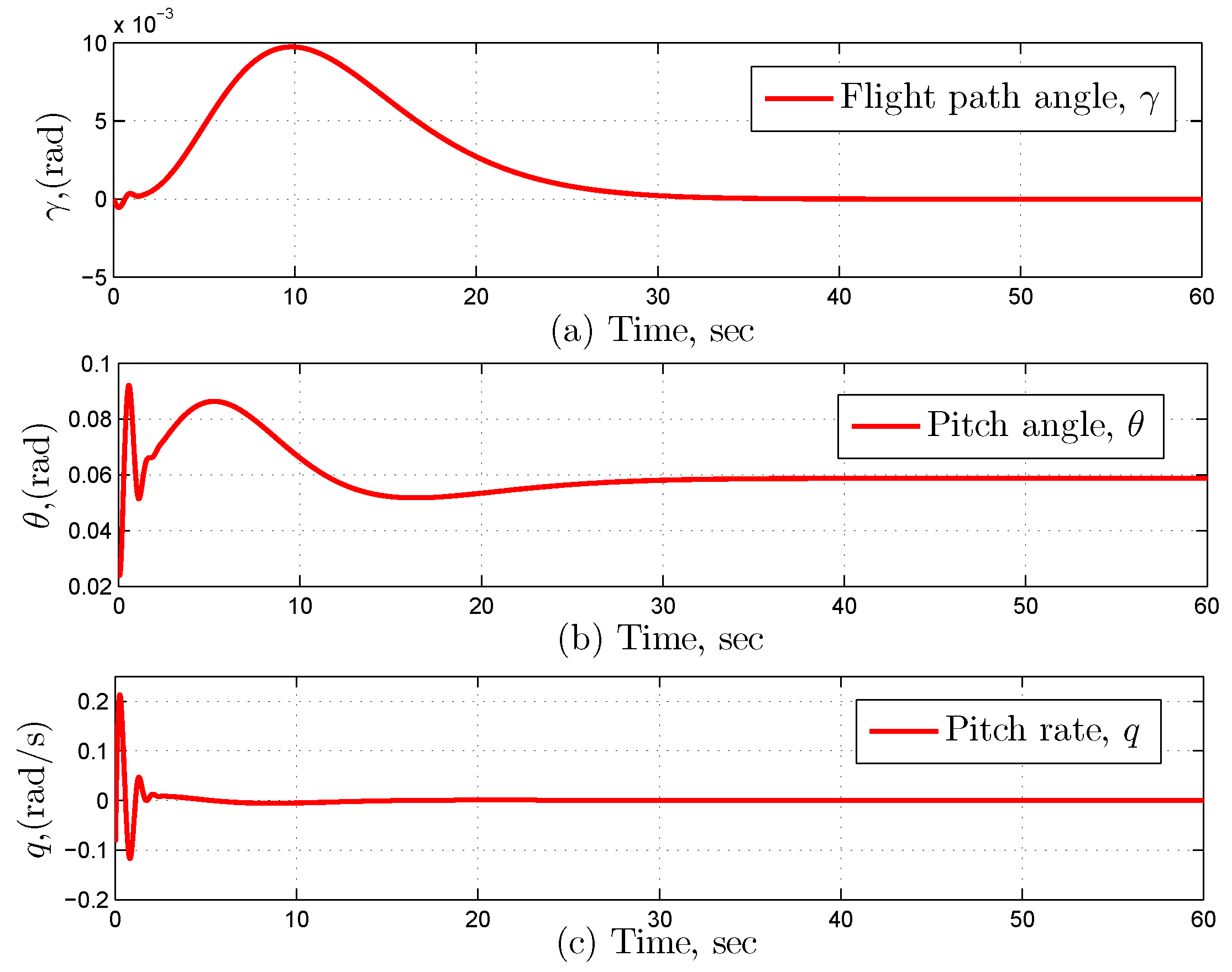
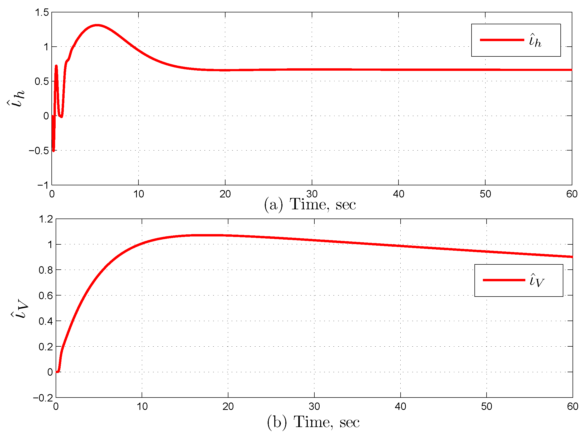
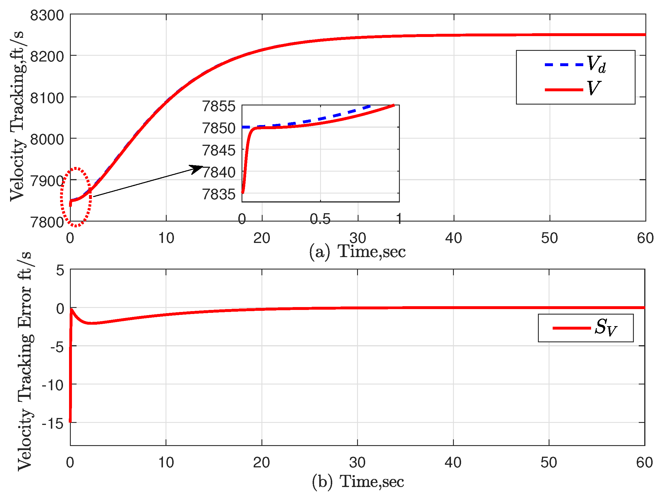
4. Simulation Results

This section presents the simulation evaluation of the proposed control stregy on the dynamic model (1) and (2) of HFA. The simulation uses the same general parameters and rated aerodynamic coefficients as the simulation model of HFA taken from [54,55]. Reference signals are generated by filtering step reference signals through a pre-filter (115) with natural frequency ${\omega }_{n_1}=0.5$, ${\omega }_{n_2}=0.3$, and $\zeta =0.85$. The reference signals for velocity and altitude are 400 ft/s and 1000 ft, respectively. In order to verify the effectiveness and adaptability of the proposed control scheme through Matlab simulation, and to demonstrate its ability to stabilize the system under different initial conditions, simulation experiments were carried out under two different initial error conditions: zero initial error condition and non-zero initial error condition, and the simulation results as shown in Figure 2, Figure 3, Figure 4, Figure 5, Figure 6, Figure 7, Figure 8, Figure 9 and Figure 10. The specific initial parameter selections are as follows:

Case 1: In this case, when $t=0$, it is assumed that the initial states of the system are $V\left(0\right)=7850$ ft/s, $h\left(0\right)=85,000$ ft, $\gamma \left(0\right)=0$ rad, $\theta \left(0\right)=0.02$ rad, and $q\left(0\right)=0$ rad/s. The initial error of the system output are zero, which means $S_V\left(0\right)=0(ft/s)$, $S_h\left(0\right)=0\left(ft\right)$.

Case 2: In this case, when $t=0$, it is assumed that the initial states of the system are $V\left(0\right)=7835$ ft/s, $h\left(0\right)=84,980$ ft, $\gamma \left(0\right)=0$ rad, $\theta \left(0\right)=0.02$ rad, and $q\left(0\right)=0$ rad/s. The initial output errors of the system are non-zero: $S_V\left(0\right)=-15(ft/s)$, $S_h\left(0\right)=-20\left(ft\right)$.

For the simulation. The design parameters are $k_V=0.55$, $a_V=1.1$, ${\gamma }_V=0$.005, ${\sigma }_V=0.1$, ${\gamma }_{\iota V}=0.01$, ${\sigma }_{\iota V}=0.5$. $k_{h1}=1$, $k_{h2}=0.1$. $k_{\gamma }=0.5$, $a_{\gamma }=1$, ${\sigma }_{\gamma }=1$, ${\gamma }_{\gamma }=1.$ $k_{\theta }=1$, $K_q=1$, $a_q=0.5$. ${\sigma }_q=0.1$, ${\gamma }_q=0.2.$ ${\gamma }_{\iota }=10$, ${\varrho }_h=0.01,$ ${\tau }_{\gamma }={\tau }_{\theta }=0.005$.

$$\begin{array}{cc}\hfill \frac{h_d}{h_c}& =\frac{{\omega }_{n_1}^2{\omega }_{n_2}^2}{{\left(p+{\omega }_{n_1}\right)}^2{\left(p+2\zeta {\omega }_{n_2}p+{\omega }_{n_2}^2\right)}^2}\hfill \\ \hfill \frac{V_d}{V_c}& =\frac{{\omega }_{n_1}^2}{p^2+2\zeta {\omega }_{n_1}p+{\omega }_{n_1}^2}\hfill \end{array}$$

(115)

Figure 2, Figure 3, Figure 4, Figure 5, Figure 6, Figure 7, Figure 8, Figure 9 and Figure 10 show the simulation results in case 1 and case 2. The simulation for Case 1 are shown in Figure 2, Figure 3, Figure 4, Figure 5, Figure 6, Figure 7 and Figure 8. Figure 2 displays the speed tracking curve and speed tracking error of the HFA. From this figure, it can be seen that, under the condition of zero initial error at $t=0$, when the system reference changes, the velocity tracking error will decrease. Due to the presence of the control system, the speed error is kept within $3 ft/s$. After about 16 s, the tracking error is less than $0.5 ft/s$ and gradually approaches zero.

Figure 3 illustrates the altitude tracking response and tracking error. From this figure, it can be seen that under the condition of zero initial error at $t=0$, when the system tracking signal changes, the altitude will have a $1.5 ft$ fluctuation in a short time, but it will be effectively controlled within 3 s, making the system tracking error gradually approach zero.

Figure 4 illustrates the response curves of the system states, including flight angle $\gamma$, pitch angle $\theta$ and pitch rate q. Figure 5 shows the response curve of the flexible structure in the system ${\eta }_1$ and ${\eta }_2$. It can be seen from the figure that when the system state changed, the flexible state quickly returns to stability after a brief oscillation. Figure 6 shows the system control signal $\Phi$, ${\delta }_e$ and quantization signal $Q(\Phi )$, $Q\left({\delta }_e\right)$. Figure 7 and Figure 8 are the system adaptive adjustment rate curves.

In order to verify the adaptability of the proposed control scheme, Figure 9 and Figure 10 show the speed and altitude tracking response curves when the system is in the case of non-zero initial error. Figure 9 is the speed response curve when the initial error of the system speed is $-15 ft/s$. It can be seen from the figure that the system error can converge and approach stability in a very short time. Figure 10 is the altitude response curve when the initial error is $-20$. It can be seen from the figure that under non-zero initial conditions, the control system can also make the system track the command signal in a short time (within 5 s) and keep it stable. Through the simulation verification of the control system under two kinds of initial tracking errors conditions, the simulation results show that the control scheme proposed in this paper has good adaptability, and can achieve satisfactory control effect under zero and non-zero initial errors. The effectiveness of the proposed control scheme is proved.

Remark 7.

It is worth noting that in practical physical systems, most control variables are also continuous variables, such as position, velocity, acceleration, etc. However, the control system simulation experiments on the Matlab platform are based on discrete time, using discrete-time simulation methods to simulate the continuous behavior of physical systems. A s long as the control system is appropriately sampled and transformed, accurate and effective simulation results can still be obtained.

Remark 8.

In order to make the proposed quantized control scheme more feasible, the design parameters can be selected using the following steps. Firstly, choose a smaller value for the time constants of the first-order low-pass filter, denoted as ${\tau }_{\gamma },{\tau }_{\theta }$, within the range of 0.001–0.1 that is practically acceptable. Secondly, after obtaining the value of $B_0$ using Equation (92), determine the values of $a_0$ using Equations (100) and (101). Thirdly, using the value of obtained in Step 2 and based on Equation (110), choose the design parameters $k_{\gamma },k_{\theta },k_q,k_V,{\gamma }_{\gamma },{\sigma }_{\gamma },{\gamma }_q,{\sigma }_q,{\gamma }_V,{\sigma }_V,{\gamma }_{\iota },{\sigma }_{\iota },{\gamma }_{\iota v},{\sigma }_{\iota v}.$

5. Conclusions

In this article, an adaptive dynamic surface input quantization control strategy is proposed for hypersonic flight aircraft with parameter uncertainties. By introducing a first-order low-pass filter in each design step, the differential explosion problem of traditional backstepping control methods is addressed and the control law structure is simplified. By online adjusting the norm of the neural network weight vector, the number of online updated parameters in the control system is reduced, and the operational efficiency is improved. The introduced hysteresis quantizer overcomes the disadvantage of the quantization accuracy deterioration when the input value decreases in the quantizer, and improves the quantization accuracy. The stability analysis proves that all signals in the closed-loop system are semi-globally uniformly bounded. Simulation results demonstrate the effectiveness of the proposed control scheme.

References

1. Moses, P.L.; Rausch, V.L.; Nguyen, L.T.; Hill, J.R. NASA hypersonic flight demonstrators—Overview, status, and future plans. Acta Astronaut. 2004, 55, 619–630. [Google Scholar] [CrossRef]
2. Sziroczak, D.; Smith, H. A review of design issues specific to hypersonic flight vehicles. Prog. Aerosp. Sci. 2016, 84, 1–28. [Google Scholar] [CrossRef] [Green Version]
3. Xu, H.; Mirmirani, M.D.; Ioannou, P.A. Adaptive sliding mode control design for a hypersonic flight vehicle. J. Guid. Control Dyn. 2004, 27, 829–838. [Google Scholar] [CrossRef]
4. Hirschel, E.H.; Weiland, C. Selected Aerothermodynamic Design Problems of Hypersonic Flight Vehicles; Springer Science & Business Media: Cham, Switzerland, 2009; Volume 229. [Google Scholar]
5. Xu, B.; Wang, D.; Sun, F.; Shi, Z. Direct neural discrete control of hypersonic flight vehicle. Nonlinear Dyn. 2012, 70, 269–278. [Google Scholar] [CrossRef]
6. Xu, B.; Gao, D.; Wang, S. Adaptive neural control based on HGO for hypersonic flight vehicles. Sci. China Inf. Sci. 2011, 54, 511–520. [Google Scholar] [CrossRef] [Green Version]
7. Xu, B.; Shi, Z. An overview on flight dynamics and control approaches for hypersonic vehicles. Sci. China Inf. Sci. 2015, 58, 1–19. [Google Scholar] [CrossRef]
8. Guoqiang, Z.; Jinkun, L. Neural network-based adaptive backstepping control for hypersonic flight vehicles with prescribed tracking performance. Math. Probl. Eng. 2015, 2015, 591789. [Google Scholar] [CrossRef] [Green Version]
9. Ma, T.N.; Xi, R.D.; Xiao, X.; Yang, Z.X. Nonlinear Extended State Observer Based Prescribed Performance Control for Quadrotor UAV with Attitude and Input Saturation Constraints. Machines 2022, 10, 551. [Google Scholar] [CrossRef]
10. Rehman, O.U.; Fidan, B.; Petersen, I.R. Uncertainty modeling and robust minimax LQR control of multivariable nonlinear systems with application to hypersonic flight. Asian J. Control 2012, 14, 1180–1193. [Google Scholar] [CrossRef]
11. Liu, J.; An, H.; Gao, Y.; Wang, C.; Wu, L. Adaptive control of hypersonic flight vehicles with limited angle-of-attack. IEEE/ASME Trans. Mechatron. 2018, 23, 883–894. [Google Scholar]
12. He, N.; Gao, Q.; Gutierrez, H.; Jiang, C.; Yang, Y.; Bi, Y. Robust adaptive dynamic surface control for hypersonic vehicles. Nonlinear Dyn. 2018, 93, 1109–1120. [Google Scholar] [CrossRef]
13. Shao, X.; Shi, Y.; Zhang, W. Fault-tolerant quantized control for flexible air-breathing hypersonic vehicles with appointed-time tracking performances. IEEE Trans. Aerosp. Electron. Syst. 2020, 57, 1261–1273. [Google Scholar] [CrossRef]
14. Qiao, H.; Meng, H.; Wang, M.; Ke, W.; Sun, J.G. Adaptive control for hypersonic vehicle with input saturation and state constraints. Aerosp. Sci. Technol. 2019, 84, 107–119. [Google Scholar] [CrossRef]
15. Rigatos, G.; Siano, P.; Selisteanu, D.; Precup, R. Nonlinear optimal control of oxygen and carbon dioxide levels in blood. Intell. Ind. Syst. 2017, 3, 61–75. [Google Scholar] [CrossRef]
16. Feng, Y.; Wu, M.; Chen, L.; Chen, X.; Cao, W.; Du, S.; Pedrycz, W. Hybrid intelligent control based on condition identification for combustion process in heating furnace of compact strip production. IEEE Trans. Ind. Electron. 2021, 69, 2790–2800. [Google Scholar] [CrossRef]
17. Kwan, C.; Lewis, F.L. Robust backstepping control of nonlinear systems using neural networks. IEEE Trans. Syst. Man Cybern. Part Syst. Hum. 2000, 30, 753–766. [Google Scholar] [CrossRef]
18. Li, Y.; Qiang, S.; Zhuang, X.; Kaynak, O. Robust and adaptive backstepping control for nonlinear systems using RBF neural networks. IEEE Trans. Neural Netw. 2004, 15, 693–701. [Google Scholar] [CrossRef]
19. Xue, G.; Lin, F.; Li, S.; Liu, H. Adaptive fuzzy finite-time backstepping control of fractional-order nonlinear systems with actuator faults via command-filtering and sliding mode technique. Inf. Sci. 2022, 600, 189–208. [Google Scholar] [CrossRef]
20. Yang, X.; Deng, W.; Yao, J. Neural adaptive dynamic surface asymptotic tracking control of hydraulic manipulators with guaranteed transient performance. IEEE Trans. Neural Netw. Learn. Syst. 2022, 1–11. [Google Scholar] [CrossRef]
21. Shi, W.; Hou, M.; Hao, M. Adaptive robust dynamic surface asymptotic tracking for uncertain strict-feedback nonlinear systems with unknown control direction. ISA Trans. 2022, 121, 95–104. [Google Scholar] [CrossRef]
22. Pan, Y.; Yu, H. Composite learning from adaptive dynamic surface control. IEEE Trans. Autom. Control 2015, 61, 2603–2609. [Google Scholar] [CrossRef]
23. Ge, J.; Wang, M.; Hong, H.; Zhao, J.; Cai, G.; Zhang, X.; Lu, P. Discrete-Time Adaptive Decentralized Control for Interconnected Multi-Machine Power Systems with Input Quantization. Machines 2022, 10, 878. [Google Scholar] [CrossRef]
24. Nie, L.; Luo, Y.; Gao, W.; Zhou, M. Rate-dependent asymmetric hysteresis modeling and robust adaptive trajectory tracking for piezoelectric micropositioning stages. Nonlinear Dyn. 2022, 108, 2023–2043. [Google Scholar] [CrossRef]
25. Zhu, G.; Li, H.; Zhang, X.; Wang, C.; Su, C.Y.; Hu, J. Adaptive consensus quantized control for a class of high-order nonlinear multi-agent systems with input hysteresis and full state constraints. IEEE/CAA J. Autom. Sin. 2022, 9, 1574–1589. [Google Scholar]
26. Gao, H.; Chen, T. A new approach to quantized feedback control systems. Automatica 2008, 44, 534–542. [Google Scholar] [CrossRef]
27. Jiang, Z.P.; Teng-Fei, L. Quantized nonlinear control—A survey. Acta Autom. Sin. 2013, 39, 1820–1830. [Google Scholar] [CrossRef]
28. Khargonekar, P.P.; Petersen, I.R.; Zhou, K. Robust stabilization of uncertain linear systems: Quadratic stabilizability and H/sup infinity/control theory. IEEE Trans. Autom. Control 1990, 35, 356–361. [Google Scholar] [CrossRef]
29. Xue, Y.; Zheng, B.C.; Yu, X. Robust sliding mode control for TS fuzzy systems via quantized state feedback. IEEE Trans. Fuzzy Syst. 2017, 26, 2261–2272. [Google Scholar] [CrossRef]
30. Lu, P.; Liu, M.; Zhang, X.; Zhu, G.; Li, Z.; Su, C.Y. Neural Network Based Adaptive Event-Triggered Control for Quadrotor Unmanned Aircraft Robotics. Machines 2022, 10, 617. [Google Scholar] [CrossRef]
31. Hayakawa, T.; Ishii, H.; Tsumura, K. Adaptive quantized control for linear uncertain discrete-time systems. Automatica 2009, 45, 692–700. [Google Scholar] [CrossRef]
32. Yu, X.; Lin, Y. Adaptive backstepping quantized control for a class of nonlinear systems. IEEE Trans. Autom. Control 2016, 62, 981–985. [Google Scholar] [CrossRef]
33. Zhang, C.; Yu, Y.; Zhou, M. Finite-time adaptive quantized motion control for hysteretic systems with application to piezoelectric-driven micropositioning stage. IEEE/ASME Trans. Mechatron. 2023, 1–12. [Google Scholar] [CrossRef]
34. Li, Y.; Liang, S.; Xu, B.; Hou, M. Predefined-time asymptotic tracking control for hypersonic flight vehicles with input quantization and faults. IEEE Trans. Aerosp. Electron. Syst. 2021, 57, 2826–2837. [Google Scholar] [CrossRef]
35. Gao, Y.; Liu, J.; Wang, Z.; Wu, L. Interval type-2 FNN-based quantized tracking control for hypersonic flight vehicles with prescribed performance. IEEE Trans. Syst. Man Cybern. Syst. 2019, 51, 1981–1993. [Google Scholar] [CrossRef]
36. Zhang, X.; Xu, H.; Chen, X.; Li, Z.; Su, C.Y. Modeling and Adaptive Output Feedback Control of Butterfly-like Hysteretic Nonlinear Systems with Creep and Their Applications. IEEE Trans. Ind. Electron. 2023, 70, 5182–5191. [Google Scholar] [CrossRef]
37. Zamfirache, I.A.; Precup, R.E.; Roman, R.C.; Petriu, E.M. Neural Network-based Control Using Actor-Critic Reinforcement Learning and Grey Wolf Optimizer with Experimental Servo System Validation. Expert Syst. Appl. 2023, 120112. [Google Scholar] [CrossRef]
38. Wang, C.; Lin, Y. Multivariable adaptive backstepping control: A norm estimation approach. IEEE Trans. Autom. Control 2011, 57, 989–995. [Google Scholar] [CrossRef]
39. Chen, B.; Liu, X.; Liu, K.; Lin, C. Direct adaptive fuzzy control of nonlinear strict-feedback systems. Automatica 2009, 45, 1530–1535. [Google Scholar] [CrossRef]
40. Chen, M.; Ge, S.S. Direct adaptive neural control for a class of uncertain nonaffine nonlinear systems based on disturbance observer. IEEE Trans. Cybern. 2012, 43, 1213–1225. [Google Scholar] [CrossRef]
41. Zhao, Q.; Lin, Y. Adaptive fuzzy dynamic surface control with prespecified tracking performance for a class of nonlinear systems. Asian J. Control 2011, 13, 1082–1091. [Google Scholar] [CrossRef]
42. Liang, H.; Zhang, Y.; Huang, T.; Ma, H. Prescribed performance cooperative control for multiagent systems with input quantization. IEEE Trans. Cybern. 2019, 50, 1810–1819. [Google Scholar] [CrossRef] [PubMed]
43. Parker, J.T.; Serrani, A.; Yurkovich, S.; Bolender, M.A.; Doman, D.B. Control-oriented modeling of an air-breathing hypersonic vehicle. J. Guid. Control Dyn. 2007, 30, 856–869. [Google Scholar] [CrossRef]
44. Xu, B.; Wang, D.; Zhang, Y.; Shi, Z. DOB-based neural control of flexible hypersonic flight vehicle considering wind effects. IEEE Trans. Ind. Electron. 2017, 64, 8676–8685. [Google Scholar] [CrossRef]
45. Bolender, M.A.; Doman, D.B. Nonlinear longitudinal dynamical model of an air-breathing hypersonic vehicle. J. Spacecr. Rocket. 2007, 44, 374–387. [Google Scholar] [CrossRef]
46. Yingwei, L.; Sundararajan, N.; Saratchandran, P. Performance evaluation of a sequential minimal radial basis function (RBF) neural network learning algorithm. IEEE Trans. Neural Netw. 1998, 9, 308–318. [Google Scholar] [CrossRef]
47. Sanner, R.M.; Slotine, J.J.E. Gaussian Networks for Direct Adaptive Control. In Proceedings of the 1991 American Control Conference, Boston, MA, USA, 26–28 June 1991; pp. 2153–2159. [Google Scholar]
48. Lewis, F.L.; Liu, K.; Yesildirek, A. Neural net robot controller with guaranteed tracking performance. IEEE Trans. Neural Netw. 1995, 6, 703–715. [Google Scholar] [CrossRef]
49. Kobayashi, H.; Ozawa, R. Adaptive neural network control of tendon-driven mechanisms with elastic tendons. Automatica 2003, 39, 1509–1519. [Google Scholar] [CrossRef]
50. Wang, C.; Wen, C.; Lin, Y.; Wang, W. Decentralized adaptive tracking control for a class of interconnected nonlinear systems with input quantization. Automatica 2017, 81, 359–368. [Google Scholar]
51. Hayakawa, T.; Ishii, H.; Tsumura, K. Adaptive quantized control for nonlinear uncertain systems. Syst. Control Lett. 2009, 58, 625–632. [Google Scholar] [CrossRef]
52. Zhou, J.; Wen, C.; Yang, G. Adaptive backstepping stabilization of nonlinear uncertain systems with quantized input signal. IEEE Trans. Autom. Control 2013, 59, 460–464. [Google Scholar] [CrossRef]
53. Tang, X.; Zhai, D.; Li, X. Adaptive fault-tolerance control based finite-time backstepping for hypersonic flight vehicle with full state constrains. Inf. Sci. 2020, 507, 53–66. [Google Scholar] [CrossRef]
54. Xu, B.; Huang, X.; Wang, D.; Sun, F. Dynamic surface control of constrained hypersonic flight models with parameter estimation and actuator compensation. Asian J. Control 2014, 16, 162–174. [Google Scholar] [CrossRef]
55. Butt, W. Observer based dynamic surface control of a hypersonic flight vehicle. Int. J. Smart Sens. Intell. Syst. 2013, 6, 664–688. [Google Scholar] [CrossRef] [Green Version]
Figure 1. Hysteresis Quantizer.
Machines 11 00630 g001
Figure 2. (a) The velocity tracking performance and (b) tracking error in Case 1.
Machines 11 00630 g002
Figure 3. (a) The altitude tracking performance and (b) tracking error in Case 1.
Machines 11 00630 g003
Figure 4. The system state response curve: flight path angle (a) γ , pitch angle (b) θ and pitch rate (c) q in Case 1.
Machines 11 00630 g004
Figure 5. Response curve of flexible states (a) η 1 and (b) η 2 in Case 1.
Machines 11 00630 g005
Figure 6. The control signals and quantized control input (a) Φ , Q ( Φ ) , (b) δ e and Q ( δ e ) in Case 1.
Machines 11 00630 g006
Figure 7. The adaptive laws of (a) υ ^ V , (b) υ ^ γ and (c) υ ^ q in Case 1.
Machines 11 00630 g007
Figure 8. The adaptive laws of (a) ι ^ h and (b) ι ^ V in Case 1.
Machines 11 00630 g008
Figure 9. (a) The velocity tracking performance and (b) tracking error in Case 2.
Machines 11 00630 g009
Figure 10. (a) The altitude tracking performance and (b) tracking error in Case 2.
Machines 11 00630 g010
Disclaimer/Publisher’s Note: The statements, opinions and data contained in all publications are solely those of the individual author(s) and contributor(s) and not of MDPI and/or the editor(s). MDPI and/or the editor(s) disclaim responsibility for any injury to people or property resulting from any ideas, methods, instructions or products referred to in the content.