
Measuring Point Planning and Fitting Optimization of the Flange and Spigot Structures of Aeroengine Rotors
by
 ,
,
Tianyi Zhou
1,2,*,
Lei Hu
1,
Xiaoxiao Jin
1,
Ting Li
1,
Yan Zhang
1,
Jianfeng Chen
2 and
Hang Gao
2 1
Shenyang Aircraft Design & Research Institute, Aviation Industry Corporation of China, Ltd., Shenyang 110035, China
2
School of Mechanical Engineering, Dalian University of Technology, Dalian 116024, China
*
Author to whom correspondence should be addressed.
Machines 2023, 11(8), 786; https://doi.org/10.3390/machines11080786
Submission received: 25 June 2023
/
Revised: 27 July 2023
/
Accepted: 28 July 2023
/
Published: 31 July 2023
(This article belongs to the Section Turbomachinery)
Abstract
:An optimized measuring point planning and fitting method for rotor flange and spigot structures was proposed to achieve precise measurement of position and pose of the aeroengine rotors during docking processes. Firstly, the impact of circumferential phase angle, distribution range angle, total number of measuring points, and number of distribution rings on measurement uncertainty was analyzed. The measuring point planning schemes for flange and spigot were proposed. Secondly, the Gauss Newton iterative solution principle considering damping factors was clarified. Subsequently, an optimized iterative reweighting method consisting of weight iterative estimation, singular value detection under the Chauvenet criterion, and clustering detection was proposed for fitting the flange annular end face. A mapping point total least squares method with practical geometric significance was proposed for fitting the spigot cylinder face. Finally, measuring and fitting experiments were performed. The singular measuring point detection methods were verified. Under the optimized fitting methods, the goodness of fit and average orthogonal distance of flange and spigot structures are 0.756 and 0.089 mm, respectively, which have higher fitting accuracy than the other traditional methods.
1. Introduction
Flange and spigot are the typical positioning structures at the end of an aeroengine rotor, realizing axis orientation, axial positioning, and radial positioning between adjacent rotors [1,2,3]. A large amount of measurement work is required during the rotor docking assembly processes, to obtain the initial position and pose of each rotor and to provide data for docking trajectories [4,5,6]. Therefore, the measuring and fitting accuracy is crucial, directly determines the assembly accuracy of the rotors, and has a significant impact on the dynamic performance of the entire engine [7,8,9,10].
Automated systems have gradually been applied in the measurement of aeroengine rotors [11,12,13,14,15]. Among these, the multi-axis precision mechanical contact measurement system and laser measurement system have the advantages of high reliability and automation [16,17,18]. A large number of point cloud coordinates are generated after measurement. The question of how to arrange the number and position of measuring points is a key issue in balancing measurement accuracy and efficiency [19,20,21,22]. Based on the measuring point planning, optimizing the corresponding fitting methods for different structures is an effective way to further reduce the uncertainty of model parameters [23,24,25]. In summary, reasonable measuring point planning and optimized fitting methods of the flange and spigot structures are important prerequisites for obtaining the rotor position and pose information quickly and accurately.
In recent years, some scholars have conducted relevant research on the measuring point planning strategy of aeroengine rotors [26,27]. Zhang et al. have proposed a redundant measuring point detection method for the measurement of rotor end faces, and the optimized algorithm improved the accuracy by 21 μm compared with the traditional least squares (LS) fitting method [28]. Zhu et al. constructed a heuristic floating forward search algorithm to efficiently find a near-optimal solution for measuring point layout [29]. Ding et al. used the eigenvalue method to process the point cloud data of the rotor end face, which has the function of excluding gross error points in the measurement points [30]. However, the existing measuring point planning methods mainly deal with integral surfaces with simple geometric shapes, and their applicability to complex spatial feature structures such as flange and spigot is limited.
With regard to the research regarding the fitting methods for typical axes and circular contours: Xie et al. established a spatial axis LS fitting model with non-cylindrical data filtered out [31]. The Limacon model is widely used in circular profile measurement to characterize eccentricity parameters [32,33]. Chetwynd et al. improved the parameter estimation method of LS fitting radius in the Limacon model [34]. Sun et al. proposed the vector projection method in cylindrical contour fitting. Compared with the traditional Limacon model, the accuracy of rotor roundness has been improved by 2.2 μm, and the accuracy of coaxiality has been improved by 9.39 μm [35,36]. Zhang et al. constructed a particle swarm optimization algorithm for fitting aeroengine rotor models based on a two-dimension laser displacement sensor, and the measurement accuracy of cylindricity error was improved by 1.768 μm compared with the traditional method [37]. Wang et al. used the equivalent homogenization processing and 3D LS method for fitting aeroengine rotor annular plane [38]. For different geometric features, researchers also carried out comparative studies on various fitting methods based on the same set of point cloud data. Song et al. compared the fitting performances of six normal line fitting methods on different types of geometries, e.g., sphere, cylinder, and ellipsoid [39]. Nouira et al. compared the fitting accuracy of different models such as LS circle, minimum area circle, maximum inscribed circle and minimum circumscribed circle, and proposed a fitting method based on a micro displacement model [40]. The above research constructed the corresponding fitting algorithms for the points with specific distribution forms, achieving higher fitting accuracy compared with traditional methods. However, few targeted combinatorial optimization algorithms have been established to meet the requirements for fitting the spatial position and pose of the rotor flange and spigot structures. Moreover, it is no longer possible to measure the flange and spigot again after the rotors are docked, so higher fitting accuracy is required in a single fitting process.
In this paper, a systematic study on measuring point planning and fitting methods for typical rotor flange and spigot structures was carried out. First, the impact of different measuring point distribution parameters on the model uncertainty was analyzed and a measuring point planning strategy was proposed. Then, the optimized iterative reweighting method for fitting flange and the mapping point total least squares method for fitting spigot were proposed, respectively. Finally, the measurement and fitting experiments were performed. The singular value point detection methods were compared and the fitting accuracy of the optimized fitting methods was verified.
2. Measuring Point Planning Method
The schematic that illustrates the measurement of the flange and spigot structures of the aeroengine rotors is shown in Figure 1. With regard to the measuring point planning of the flange annular end face. The end face description equation can be represented by zM = a1 + a2xM + a3yM in the measurement coordinate system OM-xyz. Without loss of generality, allow N measuring points Mi (xMi, yMi, zMi) distributed on the plane zM = 0 to be fitted. To simplify the calculation, the case of N = 3 is analyzed first. The measuring points M1 (0, 0, 0), M2 (xM2, 0, 0) and M3 are shown in Figure 2a. The equation of the annular end face is transformed into a1 = −(AxM + BxM + CxM)/C, a2 = −A/C, a3 = −B/C. Where A, B, and C are the model parameters of the plane general equation. The model parameter uncertainty is defined as the standard deviation of the fitting parameter and is associated with the measurement system error σM. The uncertainty of the parameter of the flange plane general equation is shown in Equations (1)–(3).
It can be calculated that when , has the minimum value, both δB and δC have the minimum values simultaneously. The uncertainty of attitude column matrix a representing the fitted normal vector of the rotor end face is shown in Equations (4)–(6).
The increase in xM2 and yM3 leads to a decrease in uncertainty δax and δay, i.e., the relative distance of the measuring points M1, M2, and M3 should be as far as possible. Then δax = δay and xM2 = ±RC and the angle among OM-Mi is 2π/3. When the calculation method is generalized to N ≥ 3, it can be concluded that the uncertainty of the end face parameters is minimized when the measuring points are uniformly distributed along the circumference.
For situations where the measurement trajectory is limited, measuring a large arc range can suffice instead of measuring the entire circle. The analysis of the impacts of the number of measuring points and the uniform distribution range on the uncertainty of the end face model parameters are necessary. The measuring points are arranged symmetrically as shown in Figure 2b. Parameter a1 determines the third-row element az in the workpiece pose column matrix a, which is an important parameter for determining the spatial angle of the end face axis (the angle between the end face normal vector and the coordinate axis OM-z). The uncertainty δa1 of parameter a1 using the LS method is calculated as Equation (7).
where N is the number of measuring points, RC is the radius of the circular path, θi is the circumferential angle of the measuring point Mi, and σM represents measurement systematic error.
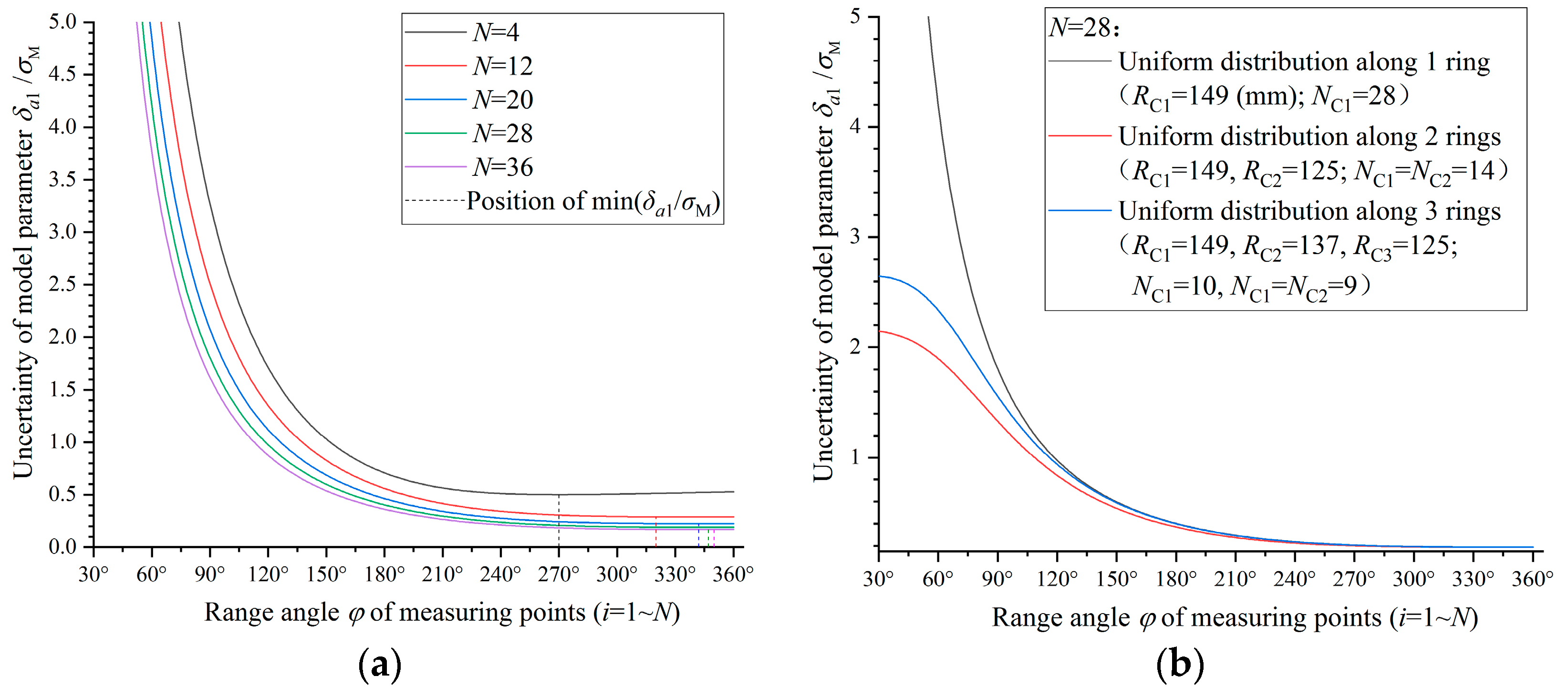
Taking the flange end face of an aeroengine low pressure turbine (LPT) mid shaft as an example, the measuring path radius RC = 149 mm. The relationship between the calculated uncertainty δa1 and the number of measuring points N/the angle of uniform distribution range φ is shown in Figure 3a. δa1 reduces significantly when φ ≥ 180°. Therefore, the measurement range should cover at least half the arc area. The reduction rate of the minimum value of the model parameter uncertainty min(δa1/σM) gradually decreases when N increases step by step in the arithmetic progression of 4, 12, 20, 28, 36. The reduction rate of min(δa1/σM) is less than 10% when N increases from 28 to 36. Taking into account the impact on measurement accuracy and efficiency, N = 28 is a reasonable value. Due to the radial width on the circular end face, the influence of the number of measuring rings distributed along multiple concentric circles/arcs is analyzed while N = 28. The uncertainty is shown in Figure 3b when RC = 149, 137 and 125 mm, respectively. When 30° ≤ φ ≤ 80°, δa1 under a multi-ring distribution reduces significantly compared with the single ring scheme and δa1 under a double-ring distribution is lower than under a three-ring distribution. Due to the limitation of the flange edge width (24 mm) in this example, when the total number of measuring points remains unchanged, the excessive rings result in a small radial spacing and a large circumferential spacing of measuring points. Therefore, the arrangement of measuring points along the double concentric rings is the optimal method and has min(δa1/σM) = 0.188. In summary, the N = 28 measuring points evenly distributed in double rings form a reasonable measuring point planning scheme, as shown in Figure 2c. Similarly, the optimized measuring point planning strategies for end faces at different positions (shown in Figure 4) in an aeroengine LPT rotor assembly are analyzed, as listed in Table 1.
With regard to the measuring point planning of the spigot cylindrical face. Without loss of generality, let N points Mproj_i (xproj_Mi, yproj_Mi, zproj_Mi) projected by the measuring points be distributed on the assumed plane zM = 0. To simplify the calculation, the case of N = 3 is analyzed first. The mapping points Mproj_1 (0, Rproj_M, 0), Mproj_2 (Rproj_Mcosθ2, Rproj_Msinθ2, 0), and Mproj_3 (Rproj_Mcosθ3, Rproj_Msinθ3, 0) are shown in Figure 2d. The coordinate uncertainty of xproj_MO and yproj_MO in the model parameters of the standard circle is shown in Equations (8) and (9).
Thus, the uncertainty δO of the center coordinates of the mapped circle is calculated as:
When ∂δO/∂θ2 = 0, the uncertainty δO has a minimum value if θ2 = θ3/2. The relationship between δO and circumferential phase angle θ3 is shown in Figure 3c. When θ2 = 2π/3, θ3 = 4π/3, δO has the minimum value 1.155σM. When the calculation method is generalized to N ≥ 3, it can be concluded that the uncertainty of the center coordinate has a minimum value when the measuring points are uniformly distributed along the circumference.
The number of points and the uniformly distributed range angle also have an impact on the uncertainty δO. The mapping points are arranged symmetrically as shown in Figure 2e. δO is calculated as Equation (11) when using the LS method.
The relationship between the uncertainty δO and the number of measuring points N/the angle of uniform distribution range φ is shown in Figure 3d. δO reduces significantly when φ ≥ 180°. Therefore, the measurement range should cover at least half the arc area. The reduction rate of the minimum value of uncertainty min(δO/σM) gradually decreases when N increases step by step in the arithmetic progression of 4, 12, 20, 28, 36, 44. The reduction rate of min(δO/σM) is less than 10% when N increases from 36 to 44. Taking into account the impact on measurement accuracy and efficiency, N = 36 is a reasonable value. Similarly, the optimized measuring point planning strategies for cylindrical faces at different positions (shown in Figure 4) in an aeroengine LPT rotor assembly are analyzed, as listed in Table 2.
3. Optimization of Fitting Algorithm
3.1. LS Principle and Gauss Newton Iterative Solution Method Considering Damping Factors
Measuring point fitting can be considered a minimization process. A set of observation values zMi are obtained under the given condition . The target is the minimization of the deviation between the values obtained from the mathematical model and the actual observation values according to a calculation rule. The LS minimization mathematical model is shown in Equation (12). The optimization fitting algorithm in Section 3.2 and Section 3.3 are all constructed based on the LS fitting principle.
The solution process of the Gauss Newton method for searching the minimum value χ2 is shown in Figure 5. The gradient of Δa = 0 when F(a + Δa) is minimized. The model parameter adjustment matrix Δa = −H−1g. The gradient vector g and Hessian matrix H are decomposed into the Jacobian matrix JLS, as shown in Equation (13).
Model parameter iteration adjustment matrix Δa is shown in Equation (14). The iteration termination target is shown in Equation (16).
where W is the weight diagonal matrix; r is the residual column vector; and ε is the iteration termination value.
The traditional Gauss Newton algorithm may fall into saddle points or iterate in wrong directions. The damping factor μ is introduced in the Levenberg–Marquardt method. Thus, the iterative adjustment matrix Δa is revised to:
The damping factor μ is determined by the adaptive coefficient λμ and the maximum diagonal element nmax of the quadratic normal matrix , as shown in Equation (18). The empirical value of λμ can be set to 0.001 in the first iteration. The direction is correct if χ2(a + Δa) < χ2(a) after iteration. Then update a + Δa→a and decrease λμ in the next iteration. Otherwise, update a and increase λμ.
3.2. Optimized Fitting Method for Flange Annular End Face
The weight wi is theoretically independent of each observation value zMi and is inversely proportional to the square of the standard uncertainty of the probability distribution function of zMi. However, the uncertainty cannot be directly calculated in practical applications. Therefore, iterative operations can be used to obtain a more accurate estimated weight. The iterative mathematical model makes the singular points deviate more significantly. Thus, singular points can be removed accurately before weighted fitting is performed again. The optimized iterative reweighted LS process for the flange annular end face is shown in Figure 6.
3.2.1. Iterative Estimation of Weights Based on Residuals
The residual Δi is approximately mapped to the weight wi. When the observed value zMi under (xMi, yMi) is very close to the model function, it causes 1/Δi to become too high. It is therefore necessary to set a reasonable upper limit value for wi:
The residual Δi obeys a normal distribution due to the influence of independent random factors. Its lower bound value λL is determined by Equation (20). To simplify operations, λL can be set as the median of absolute residual , causing 50% of the observed values to have the same weight, .
where is the estimated value of the standard deviation of the weighted observation value zMi and is the normalized mean weight value.
For the first round of fitting, i.e., the initial model parameter estimation method with equal weight, the reader can refer to Appendix A. Then, wi can be related to Δi and in the second round. The number of measuring points N for each flange is less than 100 to ensure measurement efficiency. Then, the high value of causes λL to become too high. It is difficult to distinguish observations with low from the measuring points. Therefore, it is necessary to re-estimate the weight values after obtaining the mathematical model in the last round of fitting. One should then repeat the iterations between point cloud fitting and weight estimation until the changes in the model parameters are small enough.
3.2.2. Standard Residual Singular Value Detection Based on the Chauvenet Criterion
If there is a singular value in the measuring points, its weight needs to be zeroed:
Singular points are found by calculating thresholds. Under the LS framework, the observed mean in the standard deviation formula corresponds to the estimated value. There are three elements in the parameter vector a of the flange end face. The standard deviation is estimated by Equation (23).
Threshold λ0 is set as Equation (24).
The Chauvenet criterion defines the probability of observed values occurring within the mean bandwidth range. The probability Pin of Δi occurring within the interval is shown in Equation (25).
where erf is the Gauss error function.
Set the nominal number of occurrences of singular values to v0 = NPout. The relationship between the coefficient к0 and the number of measuring points N is shown in Equation (26).
where erfinv is the Gauss inverse error function.
3.2.3. Clustering Detection
The principle of clustering detection requires that qualified observations be classified into a one-dimensional category. Their absolute deviations are relatively concentrated. Simultaneously, the deviations of singular values are far away from this category. Thus, the specified interval value is searched for in the deviation sorting and is used as the criterion for singular value determination. Cluster detection can avoid misjudgment caused by the sparsity of observation distribution.
The absolute deviations Λi are arranged in ascending order and renumbered ordinal number n:
The difference of absolute deviations between adjacent orders is:
There is a significant gap between the absolute deviations of singular values and the absolute deviations before their orders. The global criterion is that the difference of absolute deviations is higher than the typical threshold, i.e., d[n] ≥ к1dglob[n]. The local criterion is that the difference in absolute deviations is higher than the threshold generated by partial fore correlation values, i.e., d[n] ≥ к2dloc[n]. The threshold λ0 is set as Equation (30).
The global threshold dglob[n] and local threshold dloc[n] are defined as the weighted average of specific differences, shown as Equations (31) and (32). The weight decreases as the absolute deviation of the current measuring point increases and the slope is related to the number of measurement points N. The dloc[n] mainly depends on the influence of the differences of the adjacent absolute deviations. Local changes in the differences are overestimated when the absolute deviations are equal. dloc[n] should be adjusted using Equation (33). Clustering detection is self-adaptive for both dglob[n] and dloc[n] change with d[n].
3.3. Optimized Fitting Method for Spigot Cylindrical Face
The coordinates of the projection points Mproj_i on the fitted end face of the spigot measuring point Mi are calculated as Equation (34).
To obtain the spatial circle center Oproj_M(b1,b2,b3), the fitting equation after mapping is shown as Equation (35).
Compared with the traditional LS method, an optimized total least squares (TLS) method is proposed to minimize the square of the distance between the mapping of observation points and the tangent points. The tangent point is on the tangent line of the model and is orthogonal to the minimum distance vector of the measuring point and the model. Thus, TLS has more geometric significance for fitting the mapped spatial circle of the spigot, as shown in Figure 7. Due to the symmetry of the circular curve, weight estimation and singular value detection are unnecessary, and observations with relatively higher errors can also be used as conditional inputs. Referring to the definition of χ2(b), the fitted model is transformed into by shifting terms and the end face also provides a limiting condition function. The objective function of TLS is shown in Equation (36).
Different from the linear approximation solution of the minimization equation of the traditional LS method, the minimization equation of TLS is a nonlinear function regarding the model parameter vector b = (b1,b2,b3,b4)T. b can be solved through iterative compensations, and the initial estimated values in b can be calculated through the average method, as shown in Appendix A. The partial derivatives of the parameters are shown in Equations (38)–(41). The Jacobian matrix JLS contains b and requires iterative operations. Simultaneously, the operations are also constrained by the end face model, i.e., Δb3 = a1 + a2b1,fit + a3b2,fit − b3,init.
4. Measurement Experiment
Measurement and fitting experiments for an aeroengine low-pressure turbine shaft are performed. The three-axis measurement system includes: measuring head RENISHAW OMP 40-2 (a high-precision three-dimensional contact probe that can be used on coordinate measuring machines, with unidirectional repeatability of 1 μm and can be equipped with various types of measuring needles) and optical interface OMI-2T (an anti-interference infrared optical receiver for probe signals, with a detection range of 6 m). The initial position and pose of the workpiece in each experiment is randomized using an adjustment fixture. The measuring points are arranged according to the proposed planning schemes. The traditional fitting methods and the proposed optimized fitting methods are used to process the same set of measurement data, respectively. The singular point detection methods are verified and the results, such as goodness of fit and model parameter uncertainty, are compared.
4.1. Measurement and Fitting Experiment of Flange end Face
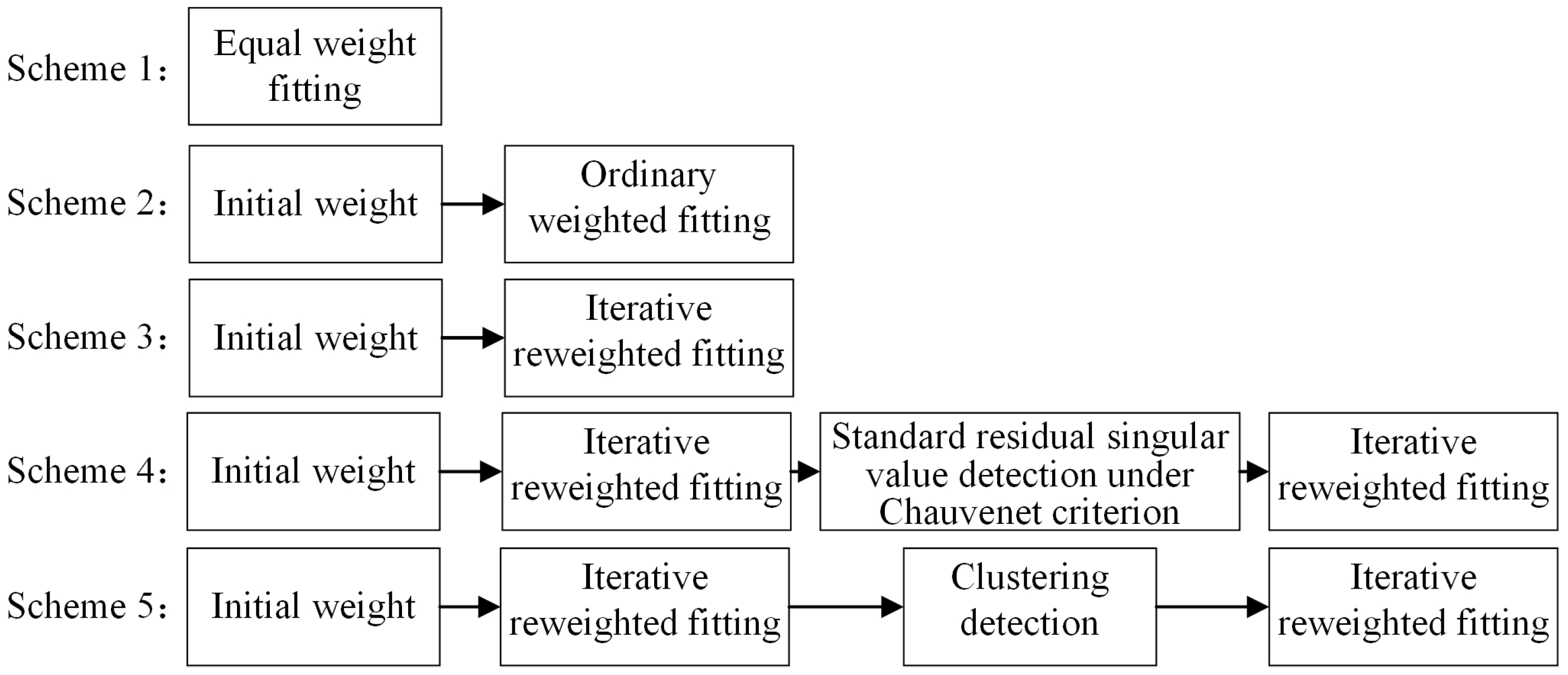
The flange end face measurement experiment is shown in Figure 8. In each measurement experiment of the rotor with random position and pose, five fitting schemes are used to fit the same coordinate data of the measurement points. The processes of different fitting schemes are shown in Figure 9.
Taking one experiment as an example, the coordinates of the measuring points are listed in Table 3. The initial estimated model parameter vector ainit is obtained after equal weight fitting and the compensation step size ∆a calculated based on the weighting times in different fitting schemes are listed in Table 4. All Δai ≤ 0.01 in the fourth iteration of weight estimation. Thus, the iteration is terminated.
The two methods for detecting singular points are compared. In the standard residual method, according to Chauvenet criterion, N = 28 makes к0 = 2.785 when the nominal probability of singular value v0 = 0.15. = 0.054 of the observed values after equal weight fitting. The threshold for this detection is λ0 = 0.151. The residual = 0.761 and = 0.743 exceed λ0. = 0.064 and λ0 = 0.179 after iterative reweighted fitting. Under this condition, = 0.894 and = 0.880 are also detected as exceeding λ0. Then, both methods determine that the measuring points i = 19, 20 are singular. In cluster detection, when the equal weight fitting is used, the difference d[27] = 0.549 in absolute deviations of measuring point i = 19 (sorting number n = 27) exceeds the local threshold к2dloc[27] = 0.348 under coefficient к2 = 2. This means that the points i = 19, 20 with greater absolute deviations show local anomalies. However, d[27] does not exceed the global threshold к1dglob[27] = 1.669 under к1 = 17. Therefore, the local anomalies are considered to be caused by the sparsity of the observed value distribution and are nonsingular points. Similarly, singular points are not detected when using ordinary weighting. If the iterative reweighting fitting is used, d[27] = 0.775 of i = 19 (n = 27) exceeds к1dglob[27] = 0.611 under к1 = 17 and к2dloc[27] = 0.163 under к2 = 2. Therefore, this position is the boundary point for distinguishing singular categories, i.e., measuring points i = 19, 20 are singular.
Due to iterative reweighting, the weight of potential singular points that deviate significantly decreases. The fitting end face is closer to the measuring points with smaller deviation. Thus, the singular points can be easier to detect. The numbers of singular points of five measurement experiments with rotor random positions and poses are listed in Table 5. Whether the measuring points have better weights has a smaller impact on the standard residual method, but a greater impact on the clustering detection method. Thus, it is necessary to perform iterative estimation of weights and model parameters before detecting singular points. The two methods have different judgment criteria, but both have achieved good results in detecting singular points and can achieve better fitting accuracy. Thus, both are reasonable methods for detecting singular points and can be used in parallel when the numerical control system has sufficient computing power.
When the singular points are removed, the weight of the model parameter vector a is re-evaluated after four iterations of reweighting. Δai ≤ 0.01 is achieved after one compensation calculation. Thus, the iteration is terminated. The fitting accuracy results of the experimental example are listed in Table 6. Because the standard residual method and clustering detection method have removed the same singular points in this experimental example, the corresponding fitting accuracy results are equal. It can be seen that the weighted fitting obtains a goodness of fit, gfit, that is less than 1.000 and closer to 1.000 than the equal weight fitting. Thus, the fitting model has a better consistency with the measuring point data. Simultaneously, the uncertainties of model parameters δa1, δa2 and δa3 decrease to varying degrees and iterative reweighting further improves fitting accuracy results compared with the ordinary weighting. The fitting after singular value detection further reduces the uncertainty of the model parameters in a small range and all uncertainties δa are less than 0.027. The fitting accuracy results of other experiments show similar patterns to this experiment example. In summary, “iterative reweighting + singular point detection (using residual method or cluster detection method) + iterative reweighting” is the optimal fitting scheme for the annular end face of the rotor flange.
4.2. Measurement and Fitting Experiment of the Spigot Cylindrical Face
The experiment in which we measured the spigot cylindrical face is shown in Figure 10. Each spigot measurement experiment is performed after the corresponding flange measurement experiment. The same coordinate data of each group of measuring points is fitted through three fitting schemes, including “OLS fitting”, “TLS fitting”, and “Iterative TLS fitting”.
The coordinates of the measuring points are listed in Table 7. The measuring points are projected towards the fitted flange end face zM = 758.4004 − 0.0243xM + 0.0300yM. The iterative compensation ∆b using LS and TLS fitting methods are calculated by the initial estimate model parameter vector binit, which are listed in Table 8. In the iterative TLS fitting, the fourth iteration is terminated for all Δbi ≤ 0.01.
TLS is a nonlinear fitting, and the Jacobian matrix JLS contains the model parameter vector b itself. The orders of magnitude of the diagonal element calculation result of covariance matrix C are too large and distort model the parameter uncertainty δb. With regard to the goodness of fit gfit, b is gathered to the same side of the model equation in TLS method and the observation value defaults to 0. This causes the calculation results of gfit to become too small to have significance in their evaluation. Therefore, the average orthogonal distance from the mapping point to the fitting model = fTLS(b)/N is used as the main accuracy evaluation indicator. The fitting accuracy results of different fitting methods of this experiment example are listed in Table 9. TLS fitting achieves smaller average orthogonal distance compared with the traditional LS fitting and can be further reduced after iterative calculation of ∆b. The fitting accuracy results of other experiments show similar patterns to this experiment example.
In summary, the iterative TLS fitting method is the optimal scheme for the rotor spigot. The final fitting equation is calculated as Equation (42).
Similarly, the TLS fitting method is used to obtain the model parameter vector of the flange reference hole: bS = [769.8345, −28.0377, 738.8523, 10.1070]. The homogeneous position and pose matrix of the low-pressure turbine shaft are shown as Equation (43).
5. Conclusions
This study focuses on the precise measurement of the position and the pose of the flange and spigot structures of rotors. The optimized measuring point planning and fitting methods are proposed and then verified through experiments. The following conclusions are drawn:
- (1)
- The equation of model parameter uncertainty δa1 that affects the end face normal vector error angle and the equation of coordinate uncertainty δO of the spigot spatial circle center are derived. The effects of the circumferential phase angle θi, distribution range angle φ, total number of measuring points N, and multiple concentric measurement paths on uncertainty are analyzed. The measuring point planning schemes for flange annular end faces and spigot cylindrical faces of the LPT rotors of an aeroengine are proposed.
- (2)
- The LS minimization criterion and Gauss Newton iterative solution principle under Levenberg Marquardt damping factors are clarified. Based on this principle, an optimized iterative reweighting method with singular values removed is proposed for fitting the flange annular end face, including processes such as residual-based weight wi iterative estimation, standard residual singular value detection under Chauvenet criterion, and clustering detection. Additionally, a mapping point TLS method with practical geometric significance is proposed for fitting the circle center of the spigot.
- (3)
- Measurement and fitting experiments on a low-pressure turbine shaft are performed. Five fitting methods for the flange annular end face are compared. When the optimized iterative reweighting method is used with singular values removed, the goodness of fit gfit = 0.756, model parameter uncertainty δa1 = 0.026, and δa2 and δa3 < 4.3 × 10⁻⁵. Simultaneously, three fitting methods for the spigot cylindrical face are compared. When the mapping point iterative TLS fitting method is used, the goodness of fit gfit = 0.011 and the average orthogonal distance = 0.089 mm. The proposed fitting methods achieve better fitting accuracy results compared with the other traditional methods.
Author Contributions
Conceptualization, T.Z.; methodology, T.Z. and H.G.; software, T.Z., L.H. and J.C.; validation, T.Z.; formal analysis, T.Z.; investigation, T.Z.; resources, T.Z. and X.J.; data curation, T.Z., L.H., X.J. and T.L.; writing—original draft preparation, T.Z.; writing—review and editing, L.H., X.J., T.L., Y.Z. and J.C.; visualization, T.Z.; supervision, H.G.; project administration, H.G. All authors have read and agreed to the published version of the manuscript.
Funding
This work is supported by Innovative Research Group Project of the National Natural Science Foundation of China (No. 51621064).
Institutional Review Board Statement
Not applicable.
Informed Consent Statement
Not applicable.
Data Availability Statement
Not applicable.
Conflicts of Interest
The authors declare no conflict of interest.
Appendix A
The estimated initial model parameters of the flange end face can be calculated as follows:
The estimated initial model parameters of the spigot cylindrical face can be calculated as follows:
References
- Liu, Y.; Zhang, M.; Sun, C.; Hu, M.; Chen, D.; Liu, Z.; Tan, J. A method to minimize stage-by-stage initial unbalance in the aero engine assembly of multistage rotors. Aerosp. Sci. Technol. 2019, 85, 270–276. [Google Scholar] [CrossRef]
- Yang, Z.; Hussain, T.; Popov, A.A.; McWilliam, S. Novel optimization technique for variation propagation control in an aero-engine assembly. Proc. Inst. Mech. Eng. Part B J. Eng. Manuf. 2011, 225, 100–111. [Google Scholar] [CrossRef]
- Nizametdinov, F.R.; Romashin, Y.S.; Berne, A.L.; Leontyev, M.K. Investigation of bending stiffness of gas turbine engine rotor flanged connection. J. Mech. 2020, 36, 729–736. [Google Scholar] [CrossRef]
- Zhou, T.; Gao, H.; Wang, X.; Li, L.; Chen, J.; Peng, C. Prediction method of aeroengine rotor assembly errors based on a novel multi-axis measuring and connecting mechanism. Machines 2022, 10, 387. [Google Scholar] [CrossRef]
- Ding, S.; He, Y.; Zheng, X. A probabilistic approach for three-dimensional variation analysis in aero-engine rotors assembly. Int. J. Aeronaut. Space 2021, 22, 1092–1105. [Google Scholar] [CrossRef]
- Hussain, T.; Yang, Z.; Popov, A.A.; McWilliam, S. Straight-build assembly optimization: A method to minimize stage-by-stage eccentricity error in the assembly of axisymmetric rigid components (two-dimensional case study). J. Manuf. Sci. Eng. 2011, 133, 031014. [Google Scholar] [CrossRef]
- Li, Z.; Zheng, X. Review of design optimization methods for turbomachinery aerodynamics. Prog. Aerosp. Sci. 2017, 93, 1–23. [Google Scholar] [CrossRef]
- Jin, S.; Ding, S.; Li, Z.; Yang, F.; Ma, X. Point-based solution using Jacobian-Torsor theory into partial parallel chains for revolving components assembly. J. Manuf. Syst. 2018, 46, 46–58. [Google Scholar] [CrossRef]
- Ma, Y.; Wang, Y.; Wang, C.; Hong, J. Interval analysis of rotor dynamic response based on Chebyshev polynomials. Chin. J. Aeronaut. 2020, 33, 2342–2356. [Google Scholar] [CrossRef]
- Satish, T.N.; Rao, A.N.V.; Nambiar, A.S.; Uma, G.; Umapathy, M.; Chandrashekhar, U.; Petley, V.U. Investigation into the development and testing of a simplex capacitance sensor for rotor tip clearance measurement in turbo machinery. Exp. Tech. 2018, 42, 575–592. [Google Scholar] [CrossRef]
- Jayaweera, N.; Webb, P.; Johnson, C. Measurement assisted robotic assembly of fabricated aero-engine components. Assem. Autom. 2010, 30, 56–65. [Google Scholar] [CrossRef]
- Wong, S.K.; Riseborough, E.; Duff, G.; Chan, K.K. Radar cross-section measurements of a full-scale aircraft duct/engine structure. IEEE Trans. Antennas Propag. 2006, 54, 2436–2441. [Google Scholar] [CrossRef]
- Garcia, I.; Przysowa, R.; Amorebieta, J.; Zubia, J. Tip-clearance measurement in the first stage of the compressor of an aircraft engine. Sensors 2016, 16, 1897. [Google Scholar] [CrossRef] [Green Version]
- Ristic, M.; Brujic, D.; Ainsworth, I. Measurement-based updating of turbine blade CAD models: A case study. Int. J. Comput. Integr. Manuf. 2004, 17, 352–363. [Google Scholar] [CrossRef]
- Burghardt, A.; Kurc, K.; Szybicki, D.; Muszynska, M.; Szczech, T. Robot-operated inspection of aircraft engine turbine rotor guide vane segment geometry. Teh. Vjesn. Tech. Gaz. 2017, 242, 345–348. [Google Scholar]
- Zhang, M.; Liu, Y.; Sun, C.; Wang, X.; Tan, J. Measurements error propagation and its sensitivity analysis in the aero-engine multistage rotor assembling process. Rev. Sci. Instrum. 2019, 90, 115003. [Google Scholar] [CrossRef]
- Sun, B.; Li, B. Laser displacement sensor in the application of aero-engine blade measurement. IEEE Sens. J. 2016, 16, 1377–1384. [Google Scholar] [CrossRef]
- Zhou, Z.; Liu, W.; Wu, Q.; Wang, Y.; Yu, B.; Yue, Y.; Zhang, J. A combined measurement method for large-size aerospace components. Sensors 2020, 20, 4843. [Google Scholar] [CrossRef] [PubMed]
- Fu, G.; Sheng, B.; Chen, G.; Luo, R.; Sheng, G.; Lu, Y. A contact on-machine measurement points’ planning method based on similarity of 3-D process element. IEEE Trans. Instrum. Meas. 2022, 71, 1–14. [Google Scholar] [CrossRef]
- Mao, Z.; Li, S.; Xu, Y.; Zeng, Q.; Zhu, K. A difference measurement points planning method for large-scale surface of aircraft. J. Beijing Univ. Aeronaut. Astronaut. 2020, 46, 1024–1031. [Google Scholar]
- Magdziak, M. Selection of the best model of distribution of measurement points in contact coordinate measurements of free-form surfaces of products. Sensors 2019, 19, 5346. [Google Scholar] [CrossRef] [PubMed] [Green Version]
- Piasecki, R. A generalization of the inhomogeneity measure for point distributions to the case of finite size objects. Phys. A 2008, 387, 5333–5341. [Google Scholar] [CrossRef] [Green Version]
- Calvo, R. Sphericity measurement through a new minimum zone algorithm with error compensation of point coordinates. Measurement 2019, 138, 291–304. [Google Scholar] [CrossRef]
- Seiler, A.; Grossmann, D.; Juettler, B. Spline surface fitting using normal data and norm-like functions. Comput. Aided Geom. Des. 2018, 64, 37–49. [Google Scholar] [CrossRef]
- Brujic, D.; Ainsworth, I.; Ristic, M. Fast and accurate NURBS fitting for reverse engineering. Int. J. Adv. Manuf. Technol. 2011, 54, 691–700. [Google Scholar] [CrossRef] [Green Version]
- Gao, F.; Pan, Z.; Zhang, X.; Li, Y.; Duan, J. An adaptive sampling method for accurate measurement of aeroengine blades. Measurement 2021, 173, 108531. [Google Scholar]
- Magdziak, M. The influence of a number of points on results of measurements of a turbine blade. Aircr. Eng. Aerosp. Technol. 2017, 89, 953–959. [Google Scholar] [CrossRef]
- Zhang, M.; Liu, Y.; Sun, C.; Wang, X.; Tan, J. Precision measurement and evaluation of flatness error for the aero-engine rotor connection surface based on convex hull theory and an improved PSO algorithm. Meas. Sci. Technol. 2020, 31, 085006. [Google Scholar] [CrossRef]
- Zhu, L.; Luo, H.; Ding, H. Optimal design of measurement point layout for workpiece localization. J. Manuf. Sci. Eng. 2008, 131, 011006–01100613. [Google Scholar] [CrossRef]
- Ding, S.; Jin, S.; Li, Z.; Wei, Z.; Yang, F. Deviation propagation model and optimization of concentricity for aero-engine rotor assembly. J. Shanghai Jiao Tong Univ. 2018, 52, 54–62. [Google Scholar]
- Xie, Z.; Jiang, Z.; Zhu, H.; Li, Z.; Lei, L.; Kong, M.; Wang, D.; Zhang, B. Research on fitting method of thread middle axis based on 3D point cloud. Acta Metrol. Sin. 2020, 41, 918–925. [Google Scholar]
- Whitehouse, D.J. Some theoretical aspects of error separation techniques in surface metrology. J. Phys. E Sci. Instrum. 1976, 9, 531–536. [Google Scholar] [CrossRef]
- Jin, S.; Fan, D.; Chen, R.; Tian, M. Method and experimental study of machine vision measurement for the roundness of rotary parts. Mach. Des. Res. 2016, 32, 117–119, 124. [Google Scholar]
- Chetwynd, D.G. High-precision measurement of small balls. J. Phys. E Sci. Instrum. 1987, 20, 1179–1187. [Google Scholar] [CrossRef]
- Sun, C.; Wang, B.; Liu, Y.; Wang, X.; Li, C.; Wang, H.; Tan, J. Design of high accuracy cylindrical profile measurement model for low-pressure turbine shaft of aero engine. Aerosp. Sci. Technol. 2019, 95, 105442. [Google Scholar] [CrossRef]
- Sun, C.; Wang, L.; Tan, J.; Zhao, B.; Tang, Y. Design of roundness measurement model with multi-systematic error for cylindrical components with large radius. Rev. Sci. Instrum. 2016, 87, 025110. [Google Scholar] [CrossRef]
- Zhang, M.; Liu, Y.; Sun, C.; Wang, X.; Tan, J. A systematic error modeling and separation method for the special cylindrical profile measurement based on 2-dimension laser displacement sensor. Rev. Sci. Instrum. 2019, 90, 105006. [Google Scholar] [CrossRef]
- Wang, J.; Sun, Q.; Yuan, B. Novel on-machine measurement system and method for flatness of large annular plane. Meas. Sci. Technol. 2020, 31, 015004. [Google Scholar] [CrossRef]
- Song, T.; Xi, F.J.; Guo, S.; Ming, Z.; Lin, Y. A comparison study of algorithms for surface normal determination based on point cloud data. Precis. Eng. 2015, 39, 47–55. [Google Scholar] [CrossRef]
- Nouira, H.; Bourdet, P. Evaluation of roundness error using a new method based on a small displacement screw. Meas. Sci. Technol. 2014, 25, 044012. [Google Scholar] [CrossRef] [Green Version]
Figure 1.
Schematic of the measurement process of the aeroengine rotor flange and spigot structures.
Figure 1.
Schematic of the measurement process of the aeroengine rotor flange and spigot structures.

Figure 2.
Schematic of measuring point distribution schemes: (a) simplified assumption of three points distributed on the flange end face; (b) points distributed uniformly on single ring on the flange end face; (c) points distributed uniformly on double rings on the flange end face; (d) simplified assumption of three points distributed on the spigot cylindrical face; (e) points distributed uniformly on the spigot cylindrical face.

Figure 3.
Relationship between measuring point distribution parameters and measurement uncertainty: (a) the influence of the number of flange measuring points and range angle; (b) the influence of the number of distribution rings of the flange measuring points; (c) the influence of the circumferential phase angle of the spigot measuring point; (d) the influence of the number of spigot measuring points and range angle.


Figure 4.
Schematic of the measurement faces on the LPT rotors of an aeroengine.

Figure 5.
Main process of LS fitting and solution method.

Figure 6.
The process of optimized iterative reweighted LS fitting method with singular values removed.
Figure 6.
The process of optimized iterative reweighted LS fitting method with singular values removed.

Figure 7.
Geometric representation of the minimization target of the mapping point TLS method.

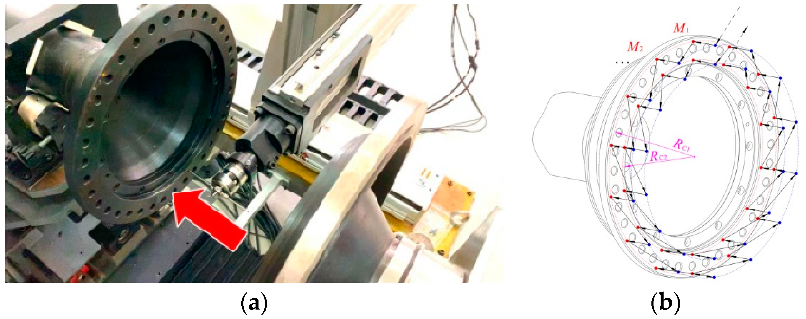
Figure 8.
Measurement experiment for the rotor flange: (a) measurement of flange annular end face; (b) measurement trajectory.
Figure 8.
Measurement experiment for the rotor flange: (a) measurement of flange annular end face; (b) measurement trajectory.

Figure 9.
Five fitting schemes in flange measurement experiments.

Figure 10.
Measurement experiment for the rotor spigot: (a) measurement of spigot cylindrical face; (b) measurement trajectory.
Figure 10.
Measurement experiment for the rotor spigot: (a) measurement of spigot cylindrical face; (b) measurement trajectory.


Table 1.
Optimized measuring point planning schemes of all end faces on the LPT rotors of an aeroengine.
Table 1.
Optimized measuring point planning schemes of all end faces on the LPT rotors of an aeroengine.
| End Faces | Fore Flange Face on the Rear Shaft/Aft Flange Face on the Cone Shaft | Fore Flange Face on the Cone Shaft/Aft Flange Face on the Mid Shaft | “Fifth” Bearing Positioning End Face on the Rear Shaft | Labyrinth Disc I Positioning End Face on the Cone Shaft | Labyrinth Disc II Positioning End Face on the Mid Shaft | Toothed Coupling Positioning End Face on the Mid Shaft |
|---|---|---|---|---|---|---|
| Total number of measuring points N | 22 | 28 | 14 | 38 | 22 | 12 |
| Distribution rings | 2 | 2 | 1 | 2 | 2 | 1 |
| Measuring path radius RC1 (mm) | 104 | 125 | 79 | 191 | 107 | 64 |
| Measuring path radius RC2 (mm) | 113 | 149 | - | 208 | 120 | - |
Table 2.
Optimized measuring point planning schemes of all cylindrical faces on the LPT rotors of an aeroengine.
Table 2.
Optimized measuring point planning schemes of all cylindrical faces on the LPT rotors of an aeroengine.
| Cylindrical Faces | Fore Spigot Face on the Rear Shaft/Aft Spigot Face on the Cone Shaft | Fore Spigot Face on the Cone Shaft/Aft Spigot Face on the Mid Shaft | “Fifth” Bearing Positioning Cylindrical Face on the Rear Shaft | Labyrinth Disc I Positioning Cylindrical Face on the Cone Shaft | Labyrinth Disc II Positioning Cylindrical Face on the Mid Shaft | Gear Coupling Positioning Cylindrical Face on the Mid Shaft |
|---|---|---|---|---|---|---|
| Total number of measuring points N | 30 | 36 | 22 | 50 | 36 | 18 |
| Spigot radius RS (mm) | 99 | 119 | 76 | 213 | 125 | 62 |
Table 3.
Coordinates of the measuring points on the flange end face.
| Point Ordinal i | Coordinate (xMi, yMi, zMi) (mm) | Point Ordinal i | Coordinate (xMi, yMi, zMi) (mm) |
|---|---|---|---|
| 1 | (779.131, −28.201, 738.614) | 15 | (755.145, −27.781, 739.189) |
| 2 | (765.561, 36.669, 740.852) | 16 | (743.757, 26.638, 741.100) |
| 3 | (725.182, 89.201, 743.466) | 17 | (709.884, 70.707, 743.266) |
| 4 | (665.992, 118.993, 745.763) | 18 | (660.228, 95.703, 745.333) |
| 5 | (599.710, 120.149, 747.419) | 19 | (604.624, 96.671, 747.502) |
| 6 | (539.475, 92.431, 748.026) | 20 | (554.089, 73.419, 748.019) |
| 7 | (497.208, 41.339, 747.523) | 21 | (518.630, 30.555, 746.707) |
| 8 | (481.281, −23.014, 745.988) | 22 | (505.269, −23.431, 745.412) |
| 9 | (494.854, −87.879, 743.753) | 23 | (516.656, −77.848, 743.528) |
| 10 | (535.232, −140.412, 741.160) | 24 | (550.530, −121.921, 741.345) |
| 11 | (594.424, −170.208, 738.866) | 25 | (600.188, −146.915, 739.493) |
| 12 | (660.704, −171.360, 737.185) | 26 | (655.788, −147.884, 738.012) |
| 13 | (720.941, −143.646, 736.614) | 27 | (706.324, −124.632, 737.485) |
| 14 | (763.209, −92.552, 737.063) | 28 | (741.783, −81.770, 737.861) |
Table 4.
Initial estimated values and iterative compensation values of the model parameters.
| Iterations | Initial Values of Model Parameters and Iterative Compensation Values |
|---|---|
| Equal weight | ainit = [758.7075, −0.0247, 0.0307] |
| First weighting | ∆a = [−0.2475, 0.0003, −0.0006] |
| Second iteration reweighting | ∆a = [−0.0677, 0.0001, −0.0001] |
| Third iteration reweighting | ∆a = [−0.0203, 0.0000, 0.0000] |
| Fourth iteration reweighting | ∆a = [0.0046, 0.0000, 0.0000] |
| Reweighting after removing singular values | ∆a = [0.0001, 0.0000, 0.0000] |
Table 5.
Number of singular points under the different pre-processing and detection methods.
| Pre-Processing before Detection | Detection Method | Experiment No. | ||||
|---|---|---|---|---|---|---|
| 1 | 2 | 3 | 4 | 5 | ||
| Equal weight | Residual method | 2 | 1 | 0 | 2 | 0 |
| Clustering detection | 0 | 0 | 0 | 1 | 0 | |
| Iterative reweighting | Residual method | 2 | 1 | 1 | 2 | 0 |
| Clustering detection | 2 | 1 | 0 | 2 | 0 | |
Table 6.
Fitting accuracy results of different fitting schemes for a rotor flange.
| Fitting Scheme | Weighted Variance χ2 | Goodness of Fit gfit | Uncertainty δa1 | Uncertainty δa2 | Uncertainty δa3 |
|---|---|---|---|---|---|
| Equal weight | 1.355 | 0.054 | 0.289 | 4.45 × 10⁻⁴ | 4.45 × 10⁻⁴ |
| Initial equal weight + ordinary weighting | 8.592 | 0.344 | 0.066 | 9.66 × 10⁻⁵ | 1.09 × 10⁻⁴ |
| Initial equal weight + iterative reweighting | 23.244 | 0.930 | 0.028 | 4.35 × 10⁻⁵ | 4.56 × 10⁻⁵ |
| Iterative reweighting + singular point detection + reweighting | 18.895 | 0.756 | 0.026 | 4.09 × 10⁻⁵ | 4.26 × 10⁻⁵ |
Table 7.
Coordinates of measuring points on the spigot cylindrical face.
| Point Ordinal i | Coordinate (xMi, yMi, zMi) (mm) | Point Ordinal i | Coordinate (xMi, yMi, zMi) (mm) |
|---|---|---|---|
| 1 | (749.407, −27.570, 735.914) | 19 | (510.816, −23.424, 741.800) |
| 2 | (747.988, −6.840, 736.496) | 20 | (512.268, −44.161, 741.056) |
| 3 | (742.961, 13.347, 737.306) | 21 | (517.289, −64.343, 740.337) |
| 4 | (734.499, 32.334, 738.070) | 22 | (525.729, −83.333, 739.604) |
| 5 | (722.886, 49.592, 738.795) | 23 | (537.342, −100.582, 738.873) |
| 6 | (708.472, 64.551, 739.561) | 24 | (551.787, −115.522, 738.089) |
| 7 | (691.649, 76.746, 740.451) | 25 | (568.603, −127.775, 737.305) |
| 8 | (672.951, 85.874, 741.211) | 26 | (587.287, −136.891, 736.484) |
| 9 | (652.969, 91.608, 741.744) | 27 | (607.274, −142.623, 735.869) |
| 10 | (632.299, 93.777, 742.380) | 28 | (627.966, −144.795, 735.212) |
| 11 | (611.534, 92.340, 742.795) | 29 | (648.684, −143.330, 734.757) |
| 12 | (591.375, 87.282, 743.212) | 30 | (668.887, −138.297, 734.422) |
| 13 | (572.349, 78.825, 743.408) | 31 | (687.876, −129.845, 734.323) |
| 14 | (555.123, 67.192, 743.357) | 32 | (705.121, −118.199, 734.216) |
| 15 | (540.129, 52.775, 743.428) | 33 | (720.110, −103.756, 734.224) |
| 16 | (527.913, 35.938, 743.246) | 34 | (732.342, −86.929, 734.493) |
| 17 | (518.756, 17.244, 742.812) | 35 | (741.472, −68.230, 734.762) |
| 18 | (513.015, −2.741, 742.426) | 36 | (747.227, −48.238, 735.204) |
Table 8.
Initial estimated values and iterative compensation values of the model parameters.
| Fitting Scheme | Initial Values of Model Parameters and Iterative Compensation Values |
|---|---|
| Initial average method estimation | binit = [630.2059, −25.6046, 742.3183, 119.3481] |
| LS fitting | ∆b= [−0.1181, 0.1368, 0.0069, −0.0001] |
| First TLS fitting | ∆b = [−0.1057, 0.1260, 0.0063, 0.0000] |
| Second TLS fitting | ∆b = [0.1119, −0.1387, −0.0069, −0.0001] |
| Third TLS fitting | ∆b = [0.0880, −0.1004, −0.0051, 0.0000] |
| Fourth TLS fitting | ∆b = [0.0005, 0.0090, 0.0002, −0.0001] |
Table 9.
Accuracy results of different fitting schemes for rotor spigot.
| Fitting Scheme | Average Orthogonal (mm) | Variance χ2 | Goodness of Fit gfit |
|---|---|---|---|
| LS fitting | 0.116 | 0.622 | 0.019 |
| Single TLS fitting | 0.105 | 0.517 | 0.016 |
| Iterative TLS fitting | 0.089 | 0.366 | 0.011 |
Disclaimer/Publisher’s Note: The statements, opinions and data contained in all publications are solely those of the individual author(s) and contributor(s) and not of MDPI and/or the editor(s). MDPI and/or the editor(s) disclaim responsibility for any injury to people or property resulting from any ideas, methods, instructions or products referred to in the content. |
© 2023 by the authors. Licensee MDPI, Basel, Switzerland. This article is an open access article distributed under the terms and conditions of the Creative Commons Attribution (CC BY) license (https://creativecommons.org/licenses/by/4.0/).
Share and Cite
MDPI and ACS Style
Zhou, T.; Hu, L.; Jin, X.; Li, T.; Zhang, Y.; Chen, J.; Gao, H. Measuring Point Planning and Fitting Optimization of the Flange and Spigot Structures of Aeroengine Rotors. Machines 2023, 11, 786. https://doi.org/10.3390/machines11080786
AMA Style
Zhou T, Hu L, Jin X, Li T, Zhang Y, Chen J, Gao H. Measuring Point Planning and Fitting Optimization of the Flange and Spigot Structures of Aeroengine Rotors. Machines. 2023; 11(8):786. https://doi.org/10.3390/machines11080786
Chicago/Turabian StyleZhou, Tianyi, Lei Hu, Xiaoxiao Jin, Ting Li, Yan Zhang, Jianfeng Chen, and Hang Gao. 2023. "Measuring Point Planning and Fitting Optimization of the Flange and Spigot Structures of Aeroengine Rotors" Machines 11, no. 8: 786. https://doi.org/10.3390/machines11080786
Note that from the first issue of 2016, this journal uses article numbers instead of page numbers. See further details here.