Hybrid Method with Parallel-Factor Theory, a Support Vector Machine, and Particle Filter Optimization for Intelligent Machinery Failure Identification

Abstract

Here, a novel hybrid method of intelligent fault identification within complex mechanical systems was proposed using parallel-factor (PARAFAC) theory and adaptive particle swarm optimization (APSO) for a support vector machine (SVM). The parallel-factor multi-scale analysis theory was studied to reconstruct tensor feature information based on a three-dimensional matrix for time, frequency, and spatial vectors. A multi-scale wavelet analysis was used to transform the original multi-channel experimental data acquired from a gearbox into a three-dimensional feature matrix of the multi-level structure. The optimal correspondence among the two-dimensional feature signals in the frequency and time domains for the different fault modes was established by the PARAFAC theory. An intelligent APSO algorithm was developed to obtain the optimal parameter structures of an SVM classifier. A comparison with the existing time–frequency analysis method showed that the proposed hybrid PARAFAC-PSO-SVM diagnosis model effectively eliminated the redundant information in the multi-dimensional tensor features but retained the important components. The PARAFAC-APSO-SVM hybrid diagnostic model achieved fast, accurate, and simple fault-classification and identification results, and could provide theoretical support for the application of the PARAFAC theory to complex mechanical fault diagnosis.

1. Introduction

Machinery plays a major role in the national economy and composes the core of the whole industrial field. The traditional manufacturing industry is constantly undergoing innovation, and advanced progress has been made as a result of the industrial revolution. This increased use of science and technology has led to the development of big data analysis, cloud computing, and artificial intelligence. To guarantee that mechanical productivity meets the requirements of modern industry and everyday life, mechanical equipment development is continuously moving towards complexity, integration, continuity, and intelligence [1,2,3]. Modern industrial machinery is produced by large-scale production systems, has rich performance indicators, and consists of a variety of mechanical components, which means that the failure of small parts can cause entire production lines, or even production plants, to stop working and producing. These failures can cause huge economic losses, can waste resources, and can even threaten the lives of staff when immediate fault diagnosis is not performed. Early health-monitoring of mechanical systems is crucial to identifying failure sources, replacing degraded mechanical components, and troubleshooting faults in a timely manner; completing these tasks can effectively reduce the risk of accidents, decrease maintenance costs, and limit hazard potential [4,5,6].

Gearboxes are devices used for transmitting motion and power and are often preferred for constant-speed applications in mechanical equipment due to their compact structures, fixed transmission ratios, and simple disassembly and installation procedures. However, due to the complexity of gearing and the fact that gearboxes often work under harsh conditions, such as high speeds and heavy loads, their primary components, such as gears, shaft systems, and bearings, usually experience varying degrees of wear and are prone to damage [7]. In the past century, many scholars and studies from around the world have focused on the special challenges associated with science and industrial technology regarding the development of original techniques for analyzing complex machinery, such as oil analysis, noise detection, vibration analysis, and non-destructive testing. Research regarding vibration-detection technology began before studies involving the other techniques; therefore, this technology is much more mature, and its application potential is the most extensive [8,9,10].

Common signal processing methods used for feature extraction for different damage and failure types include principal component analysis (PCA) techniques, classical modal analysis techniques, convolutional neural networks (CNNs), and singular-value decomposition (SVD) algorithms [11]. Previously published research regarding the methods and theory of performing feature extraction with signal analysis has effectively improved fault-feature identification and provided feasible bases for gearbox failure identification and integrity assessment. The parallel-factor decomposition model—which was first proposed in the 1970s but not used for many years due to computer storage and computing power limitations—has gained significant attention in recent decades as a new signal-processing method because of its good performance, in addition to being widely used in fields such as environmental science, clinical medicine, and image processing fields [12,13,14]. Parallel-factor analysis methods are most commonly used for 3D fluorescence spectroscopy within the environmental science and resource utilization disciplines. The theory behind the parallel-factor method has been improved and its associated techniques have gradually matured alongside its expansion into fields outside of chemistry [15]. Sidropoulos developed direct sequence–code division multiple access (DS–CDMA) systems by applying the parallel-factor theory to signal processing [16]. Liang [17] proposed a new blind model by using the parallel-factor (PARAFAC) code division of multiple-access systems for blind signal detection in CDMA systems. Yang [18] used the tensor singular spectrum to analyze the underdetermined observed signals for blind source separation.

In recent years, scholars have begun to investigate PARAFAC methods for degradation monitoring of mechanical systems. Zhang et al. [19] established the parallel-factor algorithm for integrity assessments of wind turbines. The fault information acquired by the data acquisition and monitoring system was used to conduct effective wind farm condition monitoring. Wang [20] used the PARAFAC method to reconstruct multi-source bearing fault signals. Fault-condition classification of engineering systems was achieved by combining principal component analysis with the alternating least squares method. In general, matrix decomposition is not unique unless a constraining condition, such as orthogonality, the Toeplitz condition, or the constant mode, is imposed. However, these harsh constraints are not satisfied in practical applications. A new method must be sought to solve this problem. Unlike traditional 2D signal processing methods, the PARAFAC method can decompose 3D and multidimensional signals to obtain unique solutions under relatively loose constraints. The PARAFAC analysis method can uncover the underlying structure and reflect the essential characteristics of high-dimensional data and can therefore efficiently utilize multi-channel signals for fault detection. Therefore, research regarding the use of a PARAFAC-based method for mechanical fault diagnosis was conducted during this study.

In light of the above, it is urgent to develop theories and methods for mechanical fault diagnosis under non-stationary operating conditions to ensure that modern industrial production processes achieve intelligence, digital monitoring and diagnostic prediction. This issue has become a technical limitation and is a recognized challenge when applying fault-diagnosis technology to key mechanical equipment in engineering practice. This paper focuses on intelligent techniques of vibration signal analysis. The goal of this paper is to propose an intelligent hybrid method, based on parallel-factor theory for the adaptive diagnosis of nonstationary fault modes, that uses adaptive particle swarm optimization (APSO) with a support vector machine (SVM) to improve fault-diagnosis intelligence and accuracy.

2. Optimized Hybrid PARAFAC–APSO–SVM Model

2.1. Parallel Factors Model

The essence of the PARAFAC structure is the low-order multi-decomposition process of the multi-dimensional matrices that represent multiple linear models. The parallel-factor decomposition theory is described next.

The three-dimensional matrix, $\mathrm{X}\in {\mathrm{C}}^{\mathrm{P}\times \mathrm{Q}\times \mathrm{N}}$, was subjected to PARAFAC decomposition with scalar expressions, as shown in Equation (1):

$${\mathrm{X}}_{\mathrm{p},\mathrm{q},\mathrm{n}}={\sum }_{\mathrm{m}=1}^{\mathrm{M}}{\mathrm{A}}_{\mathrm{p},\mathrm{m}}{\mathrm{B}}_{\mathrm{q},\mathrm{m}}{\mathrm{C}}_{\mathrm{n},\mathrm{m}}+{\mathrm{E}}_{\mathrm{p},\mathrm{q},\mathrm{n}}.$$

(1)

In Equation (1), the variable ranges are p $=\mathrm{1,2},\dots \mathrm{P},\mathrm{q}=\mathrm{1,2},\dots \mathrm{Q},\mathrm{n}=\mathrm{1,2},\dots \mathrm{N},\mathrm{and} \mathrm{m}=\mathrm{1,2},$… M. The 2D moments, $\mathrm{A},\mathrm{B} \mathrm{and} \mathrm{C}$, are the loading matrices of the PR multi-level model. 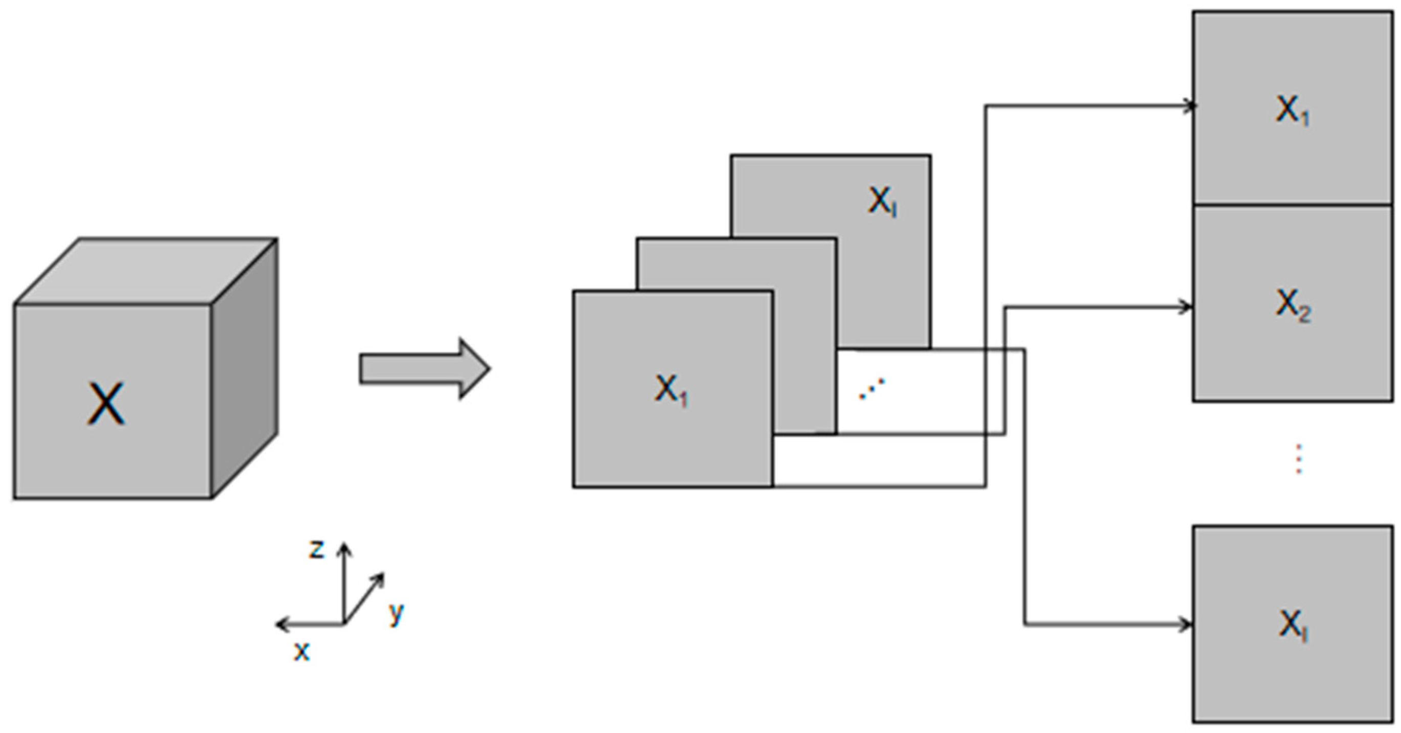The sets $\mathrm{A}\in {\mathrm{C}}^{\mathrm{P}\times \mathrm{M}}$, $\mathrm{B}\in {\mathrm{C}}^{\mathrm{Q}\times \mathrm{M}}$, $\mathrm{C}\in {\mathrm{C}}^{\mathrm{N}\times \mathrm{M}},\mathrm{and} \mathrm{E}\in {\mathrm{C}}^{\mathrm{P}\times \mathrm{Q}\times \mathrm{N}}$ are noise matrices. The low-order multi-decomposition process was enlarged to a higher dimension. The number of dimensions increased, which caused the degrees of freedom of the elements in the matrix to also increase. The abstraction process became much more complicated. Only 3D matrices were investigated during this study. In practice, the 3D model can also be used to intercept profiles from different directions by using the 2D set matrix, which is equivalent to the 3D-model representation. Figure 1 presents the 2D set matrix along the x-axis direction within the PARAFAC model.

The primary formula used in the PARAFAC model is expressed in Equation (2):

$$\left\{\begin{array}{c}{\mathrm{X}}_{\mathrm{p}::}=\mathrm{B}{\mathrm{D}}_{\mathrm{p}}\left(\mathrm{A}\right){\mathrm{C}}^{\mathrm{T}}+{\mathrm{E}}_{\mathrm{p}::}\\ {\mathrm{X}}_{:\mathrm{q}:}=\mathrm{A}{\mathrm{D}}_{\mathrm{q}}\left(\mathrm{B}\right){\mathrm{C}}^{\mathrm{T}}+{\mathrm{E}}_{:\mathrm{q}:}.\\ {\mathrm{X}}_{\mathrm{n}::}=\mathrm{A}{\mathrm{D}}_{\mathrm{i}}\left(\mathrm{C}\right){\mathrm{B}}^{\mathrm{T}}+{\mathrm{E}}_{::\mathrm{n}}\end{array}\right.$$

(2)

In Equation (2), the set ${\mathrm{D}}_{\mathrm{p}}\left(\mathrm{A}\right)$ is the element of the pth row of extracted matrix A and is constructed as a diagonal sub-matrix. The parallel-factor model has significant advantages over 2D matrix decomposition in that it allows the fuzzy decompositions of the column and scale to be unique in the absence of any other constraints. In terms of the discriminating conditions of the PARAFAC set, the definition of the k-order matrix is introduced as the rank of set A. Set A consists of independent columns when, and only when, the total number of columns is at least equal to r, which is defined below:

$${\mathrm{r}}_{\mathrm{A}}=\mathrm{O}\mathrm{r}\mathrm{d}\mathrm{e}\mathrm{r}\left(\mathrm{A}\right)=\mathrm{r}.$$

(3)

The parameter k is the number of independent column vectors in set matrix A. The required condition for the order of set matrix A is ${\mathrm{k}}_{\mathrm{A}}=\mathrm{k}, \mathrm{where} {\mathrm{k}}_{\mathrm{A}}\le {\mathrm{r}}_{\mathrm{A}}\le \mathrm{m}\mathrm{i}\mathrm{n}\left\{\mathrm{P},\mathrm{M}\right\} \mathrm{and} \forall \mathrm{A}$.

There is only one solution for the three sub-matrices of the PR decomposition after both the scale and column transformations. It is required that the k-orders of matrices A, B, and C satisfy ${\mathrm{k}}_{\mathrm{A}}+{\mathrm{k}}_{\mathrm{B}}+{\mathrm{k}}_{\mathrm{C}}\ge 2(\mathrm{M}+1)$. The sufficient condition for discriminability of the multi-decomposition PARAFAC model is presented as follows:

$$\mathrm{m}\mathrm{i}\mathrm{n}\left\{\mathrm{P},\mathrm{M}\right\}+\mathrm{m}\mathrm{i}\mathrm{n}\left\{\mathrm{Q},\mathrm{M}\right\}+\mathrm{m}\mathrm{i}\mathrm{n}\left\{\mathrm{N},\mathrm{M}\right\}\ge 2\mathrm{M}+3.$$

(4)

2.2. Support Vector Machine Theory

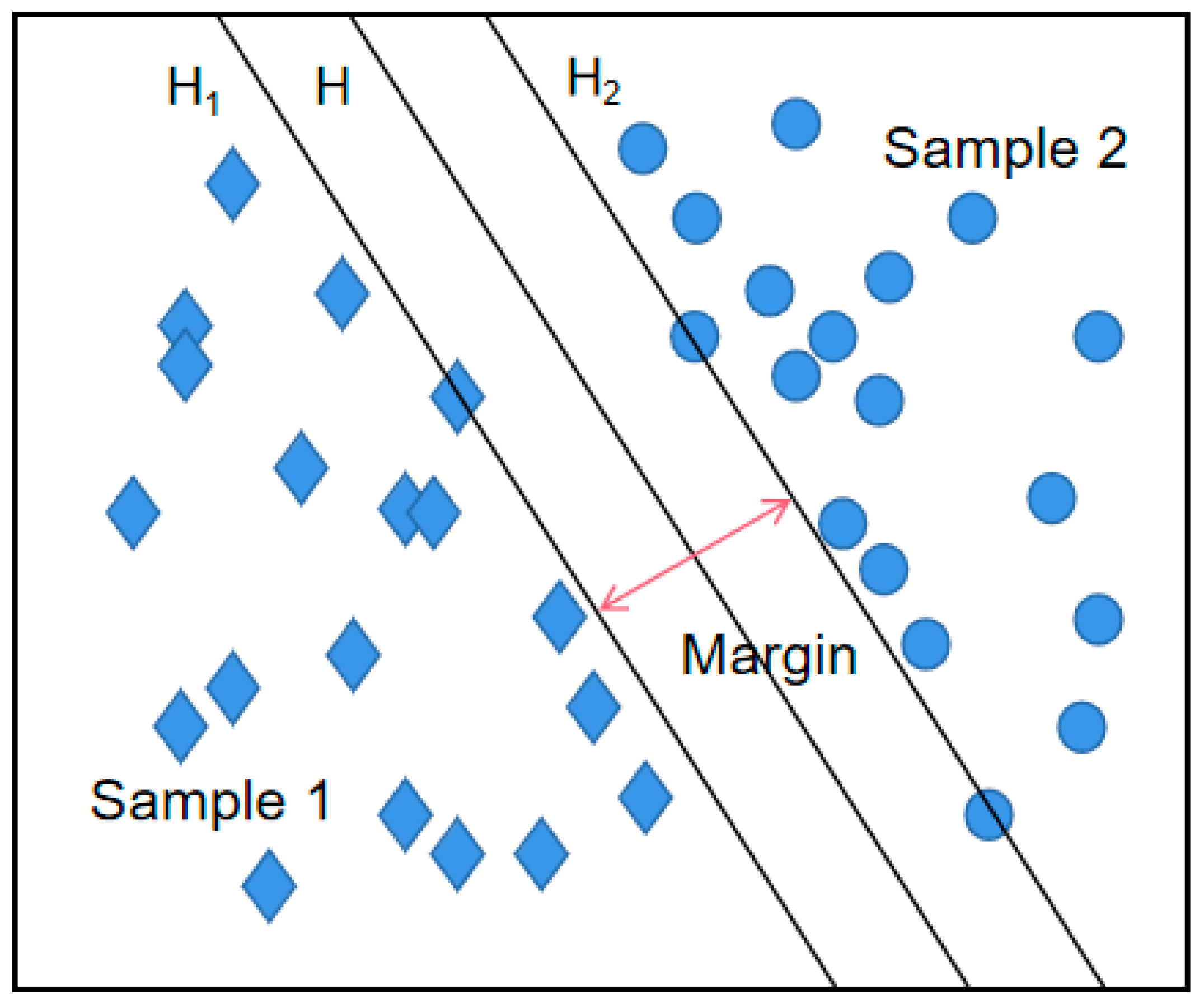
Support vector machines were invented as a result of the binary classification problem, which was proposed as a linear classifier model to construct binary feature spaces with the maximum interval. The interval between the training data sets is maximized by establishing a divided hyperplane using optimization theory, as shown in Figure 2.

The training data set is supposed to be ${(\mathrm{t}}_{\mathrm{i}}{,\mathrm{f}}_{\mathrm{i}}), \mathrm{where} =\mathrm{1,2}\cdots ,\mathrm{N}$. The input data and learning objectives in the classification problem are given as $\mathrm{T}=\left\{{\mathrm{T}}_1,\dots ,{\mathrm{T}}_{\mathrm{N}}\right\}$ and $\mathrm{f}=\left\{{\mathrm{f}}_1,\dots ,{\mathrm{f}}_{\mathrm{N}}\right\}$, respectively. The multiple features included in the input data construct the feature space according to ${\mathrm{t}}_{\mathrm{i}}\in {\mathrm{R}}^{\mathrm{n}}$. The updated objectives are bi-category objectives: $\mathrm{f}\in \left\{-\mathrm{1,1}\right\}$. The hyperplane exists and is regarded as the decision boundary in the feature space in which the input data are located, and the updated optimization objectives are divided into two classes. The distance from the geometric location of any data point to the hyperplane is greater than or equal to 1. The decision boundary is defined according to Equation (5):

$$(\mathrm{t}·\mathsf{\omega }+\mathrm{b}=0).$$

(5)

The condition that the separation line correctly classifies all the sample data as one of two types satisfies the separation interval. Therefore, Equation (5) can be transformed into

$${\mathrm{F}}_{\mathrm{i}}\left[\left({\mathrm{t}}_{\mathrm{i}}·\mathsf{\omega }\right)+\mathrm{b}\right]\ge 1,\mathrm{i}=\mathrm{1,2},\cdots ,\mathrm{N}.$$

(6)

At this point, the classification interval margin is equal to $2/{‖\mathsf{\omega }‖}^2$. The optimal hyperplane is constructed by a transformation into a minimum problem with constraints. We first assume that a hyperplane has a parameter that is a geometric interval between the plane and the data set. The constraint function is used to control the geometric interval. When the geometric interval is smaller, the hyperplane is better. Thus, the problem of finding the optimal plane can be transformed into the problem of finding its constraint optimization problem by finding the minimum values of variables $\mathsf{\omega }$ and b to produce the minimum value of parameter $‖\mathsf{\omega }‖$. The final classification hyperplane, which is obtained after training the sample data, is determined by the sample data points at the limit surface, i.e., the training sample points on H₁ and H₂ are called support vectors.

The disadvantage of using the hard-margin SVM to solve linear non-separable problems is that it easily generates classification errors. Therefore, a loss function based on margin maximization is introduced in the proposition of a novel optimization method. To find the maximum interval and minimize the number of misclassifications or serious classification errors, the objective function must be adjusted by introducing a slack variable, $\mathsf{\xi }$, to reduce the constraint and by adding a penalty factor, $\mathrm{C}$, to balance the $\mathsf{\xi }$ values, which control the optimization tendency. The SVM expression can then be obtained, as shown below:

$${}_{\mathsf{\omega },\mathrm{b}}{}^{\mathrm{m}\mathrm{i}\mathrm{n}}\frac{1}{2}{‖\mathsf{\omega }‖}^2+\mathrm{C}{\sum }_{\mathrm{i}=1}^{\mathrm{N}}{\mathsf{\xi }}_{\mathrm{i}},$$

(7)

$${\mathrm{s}.\mathrm{t}.\mathrm{f}}_{\mathrm{i}}\left({\mathrm{t}}_{\mathrm{i}}\cdot \mathsf{\omega }+\mathrm{b}\right)\ge 1-{\mathsf{\xi }}_{\mathrm{i}}.$$

(8)

A nonlinear SVM can be obtained by mapping the original input data into the high-dimensional feature space by using a nonlinear function in a linear SVM. However, the nonlinear SVM has some optimization problems. By introducing the Lagrange function, Equations (7) and (8) can be transformed into a dyadic expression according to the Karush–Kuhn–Tucker (KKT) theory:

$${}_{\mathsf{\alpha }}{}^{\mathrm{m}\mathrm{a}\mathrm{x}}{\sum }_{\mathrm{i}}^{\mathrm{N}}{\mathsf{\alpha }}_{\mathrm{i}}-\frac{1}{2}{\sum }_{\mathrm{i}}^{\mathrm{N}}{\sum }_{\mathrm{j}}^{\mathrm{N}}{\mathsf{\alpha }}_{\mathrm{i}}{\mathsf{\alpha }}_{\mathrm{j}}{\mathrm{f}}_{\mathrm{i}}{\mathrm{f}}_{\mathrm{j}}\mathrm{K}\left({\mathrm{t}}_{\mathrm{i}},{\mathrm{t}}_{\mathrm{j}}\right)$$

(9)

$$\mathrm{s}.\mathrm{t}.{\sum }_{\mathrm{i}}^{\mathrm{N}}{\mathsf{\alpha }}_{\mathrm{i}}{\mathrm{f}}_{\mathrm{i}}=0,{\mathsf{\alpha }}_{\mathrm{i}}\in \left[0,\mathrm{C}\right].$$

(10)

In Equations (9) and (10), the parameter $\mathsf{\alpha }$ is the KKT multiplier that the Lagrange multiplier uses to impose the inequality constraint. The Gaussian radial basis kernel is universally applicable, so it was chosen as the kernel function. The unique parameter $\mathsf{\sigma }$ must be set up according to Equation (11):

$$\mathrm{K}\left({\mathrm{t}}_{\mathrm{i}},{\mathrm{f}}_{\mathrm{i}}\right)=\mathrm{e}\mathrm{x}\mathrm{p}\left(-\frac{{‖{\mathrm{t}}_{\mathrm{i}}-{\mathrm{f}}_{\mathrm{i}}‖}^2}{2{\mathsf{\sigma }}^2}\right).$$

(11)

The objective function can thus be ultimately expressed by Equation (12):

$$\mathrm{H}\left(\mathrm{t}\right)={\sum }_{\mathrm{i}=1}^{\mathrm{N}}{\mathsf{\alpha }}_{\mathrm{i}}{\mathrm{f}}_{\mathrm{i}}\mathrm{K}\left({\mathrm{t}}_{\mathrm{i}},{\mathrm{f}}_{\mathrm{i}}\right)+\mathrm{b}.$$

(12)

2.3. Improved APSO Algorithm

The traditional particle swarm algorithm finds the optimal particles by learning from the particles’ historical experience $\left({\mathrm{p}}^{\mathrm{best}}\right)$ and population experience $\left({\mathrm{g}}^{\mathrm{best}}\right)$; this algorithm has been widely used because of its high computational speed and robustness. The important SVM parameters, $\mathrm{C}$ and $\mathsf{\sigma }$, must be optimized to establish the optimal decision boundaries of the 3D feature space in an SVM. $\mathrm{C}$ is used to control the penalties of the misclassified training examples and $\mathsf{\sigma }$ is the kernel function parameter. A new particle-velocity updating strategy for PSO is proposed according to the definition of the core PSO search formula:

$${\mathrm{v}}_{\mathrm{i}\mathrm{d}}\left(\mathrm{t}+1\right)=\mathrm{w}\mathrm{v}\left(\mathrm{t}\right)+{\mathrm{c}}_1{\mathrm{r}}_1\left(\mathrm{p}{\mathrm{b}\mathrm{e}\mathrm{s}\mathrm{t}}_{\mathrm{i}\mathrm{d}}-\mathrm{x}\left(\mathrm{t}\right)\right)+{\mathrm{c}}_2{\mathrm{r}}_2\left(\mathrm{g}{\mathrm{b}\mathrm{e}\mathrm{s}\mathrm{t}}_{\mathrm{i}\mathrm{d}}-\mathrm{x}\left(\mathrm{t}\right)\right),$$

(13)

$${\mathrm{x}}_{\mathrm{i}\mathrm{d}}\left(\mathrm{t}\right)={\mathrm{x}}_{\mathrm{i}\mathrm{d}}\left(\mathrm{t}\right)+{\mathrm{v}}_{\mathrm{i}\mathrm{d}}\left(\mathrm{t}+1\right).$$

(14)

In Equations (13) and (14), ${\mathsf{\nu }}_{\mathrm{i}\mathrm{d}}$ and ${\mathrm{x}}_{\mathrm{i}\mathrm{d}}$ represent the particle velocity and generation, respectively. The variable representing the inertia weight $\left(\mathrm{w}\right)$ decreases linearly with successive iterations; ${\mathrm{c}}_1$ and ${\mathrm{c}}_2$ are the learning factors; ${\mathrm{r}}_1$ and ${\mathrm{r}}_2$ are mutually independent, arbitrary numbers between 0 and 1. The particles of the APSO algorithm are updated to pursue the optimal values of the particles in the neighborhood and to update their velocities. The distances between a specific particle and other particles are computed one-by-one during each iteration; l_mn represents the distance between the $m^{th}$ particle and the $n^{th}$ particle. The maximum value of l_mn is l_max. The specific value $l_{mn}/l_{max}$ can also be obtained. The value of the threshold $\left(\mathsf{\theta }\right)$ is adaptively adjustable according to the number of cycles; $\mathsf{\theta }$ is defined below:

$$\mathsf{\theta }=\frac{0.3\mathrm{g}+0.6{\mathrm{g}}_{\mathrm{m}\mathrm{a}\mathrm{x}}}{{\mathrm{g}}_{\mathrm{m}\mathrm{a}\mathrm{x}}}.$$

(15)

In Equation (15), $\mathrm{g}$ is the cycle index with a maximum value of ${\mathrm{g}}_{\mathrm{m}\mathrm{a}\mathrm{x}}$. When $\mathsf{\theta }$ is equal to 0.9 and $l_{mn}/l_{max}$ is less than $\mathsf{\theta }$, the $n^{th}$ particle is supposed to be near the $m^{th}$ particle. The velocity of the particle is refreshed by an updated learning factor c₃, and a random parameter, r₃. Equation (13) can then be rewritten as

$${\mathrm{v}}_{\mathrm{i}\mathrm{d}}\left(\mathrm{t}+1\right)=\mathrm{w}\mathrm{v}\left(\mathrm{t}\right)+{\mathrm{c}}_1{\mathrm{r}}_1\left(\mathrm{p}{\mathrm{b}\mathrm{e}\mathrm{s}\mathrm{t}}_{\mathrm{i}\mathrm{d}}-\mathrm{x}\left(\mathrm{t}\right)\right)+{\mathrm{c}}_2{\mathrm{r}}_2\left(\mathrm{g}{\mathrm{b}\mathrm{e}\mathrm{s}\mathrm{t}}_{\mathrm{i}\mathrm{d}}-\mathrm{x}\left(\mathrm{t}\right)\right)+{\mathrm{c}}_3{\mathrm{r}}_3\left(\mathrm{q}{\mathrm{b}\mathrm{e}\mathrm{s}\mathrm{t}}_{\mathrm{i}\mathrm{d}}-\mathrm{x}\left(\mathrm{t}\right)\right).$$

(16)

If $\mathsf{\theta }$ is greater than 0.9 or if $l_{mn}/l_{max}$ is greater than $\mathsf{\theta }$, then Equation (13) is used to refresh the particle velocity.

Conventional PSO applies the inertia weights along with linear reduction to alter the step length in the search process, which causes the optimization toward the extreme point to gradually converge. A shortcoming of conventional PSO is that it is prone to falling into local optima. An improved PSO algorithm, the APSO algorithm, is proposed to address the drawback of local convergence without the optimization inherent to the conventional PSO. The weights, $\mathrm{w}$, of the APSO algorithm decrease according to an S-shaped function so that ${\mathrm{w}}_{\mathrm{i}}$ changes dynamically. At the beginning of the optimization search when using the APSO algorithm, the original value of ${\mathrm{w}}_{\mathrm{i}}$ is set as a large value to facilitate global optimization. At the end of the optimization search process, ${\mathrm{w}}_{\mathrm{i}}$ is evaluated as a smaller value so it can conduct the optimization search process. This improved strategy for updating ${\mathrm{w}}_{\mathrm{i}}$ in the APSO algorithm is achieved by the definition below:

$${\mathrm{w}}_{\mathrm{i}}=\frac{{\mathrm{w}}_{\mathrm{i}\mathrm{m}\mathrm{a}\mathrm{x}}-{\mathrm{w}}_{\mathrm{i}\mathrm{m}\mathrm{i}\mathrm{n}}}{1+\mathrm{e}\mathrm{x}\mathrm{p}\left(2\mathrm{e}\mathrm{t}/{\mathrm{t}}_{\mathrm{m}}-\mathrm{e}\right)}.$$

(17)

2.4. SVM Optimization with the APSO Algorithm

The APSO algorithm primarily optimizes the penalty coefficients of SVM functions and the parameters of kernel functions, that is, a slack variable, $\mathsf{\xi }$, which reduces the constraint, and a penalty factor, $\mathrm{C}$, which determines the penalty degree for the model complexity and fitting bias. These two variables have significant impacts on the SVM regression model. Values that are both too large and too small can affect the system’s generalization performance. The kernel function parameters precisely define the structure of the high-dimensional space. The optimal parameters must be selected to ensure the generalization capability of the system. The standard for determining the optimal parameters of an SVM classifier is based on there being the same number of iterations for both the improved and non-improved SVM. The higher the SVM correction rate, the better the parameters. The optimal parameters are selected based on higher SVM classification correction rates.

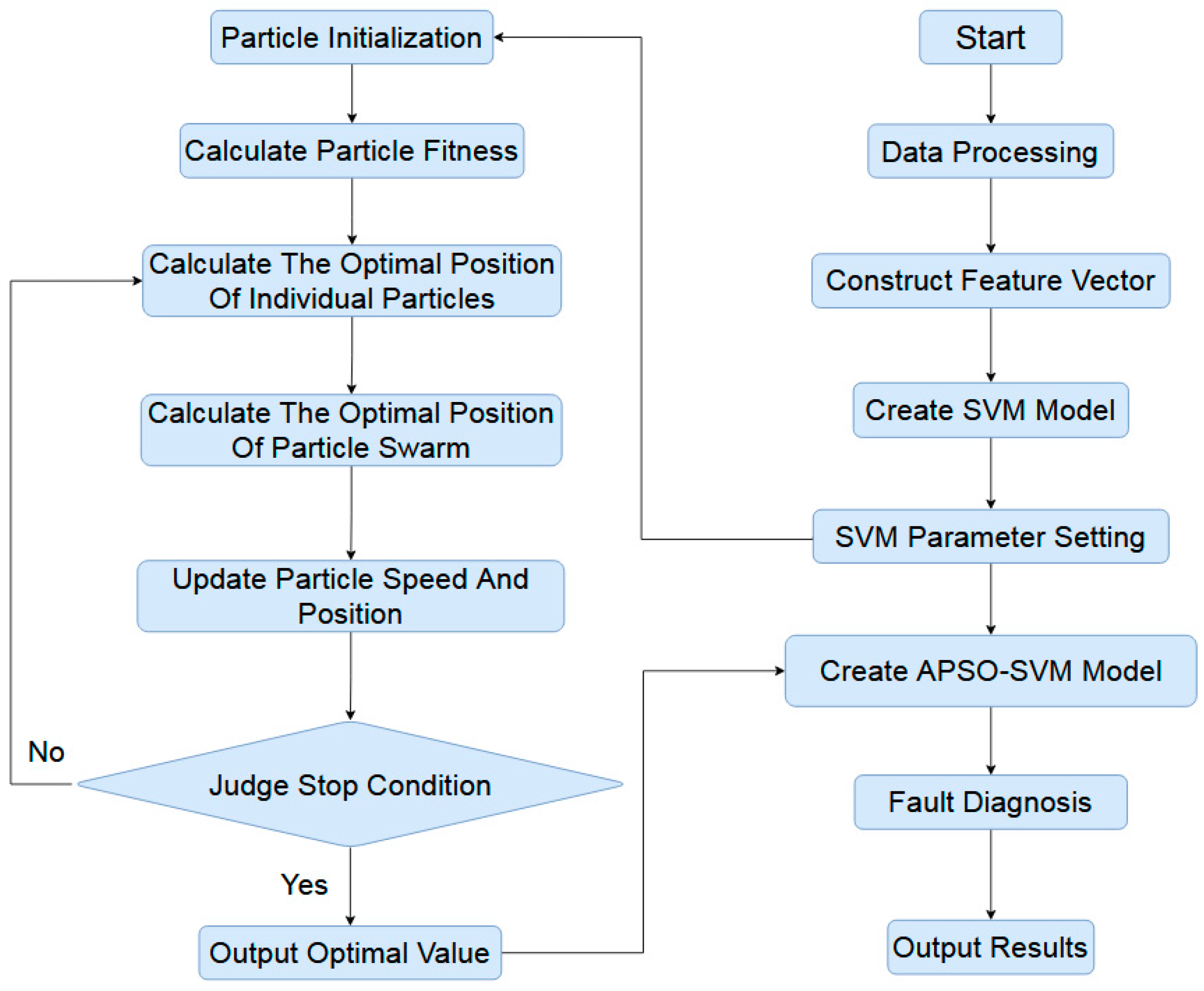
A flowchart depicting the use of the APSO algorithm to optimize the SVM classifiers is shown in Figure 3. The procedure consists of five primary steps.

• The parameters in the APSO algorithm are initialized; these include the number of particles, the initial particle positions, the number of evolutionary generations, the acceleration factor, and the maximum loop value.
• The fitness values of the particles are computed and compared based on a given objective function. The APSO algorithm uses the objective function in Equation (9) as a self-adjusting fitness function.
• The fitness values of the individual particles with optimal positions are obtained and the optimal positions of all the particles are refreshed.
• The fitness values for the local optimal positions of the particles are compared to the fitness value of the particle’s global optimal position to obtain the new global optimal particle positions.
• Equations (13)–(16) are used to refresh the velocities and positions of the particles. If the loop has finished or the accuracy requirement has been met, the optimal values are output and substituted into the SVM. Otherwise, the conditional requirement has not been met, and the process returns to Step (2) and continues from there.

3. Experimental System for the Gearbox

Five fault modes $\left(FMs\right)$ were set up for a gearbox system to simulate gearbox failure; these fault modes consist of a normal gear mode $\left({FM}_1\right)$ and four broken gear modes $\left({FM}_2,{FM}_3,{FM}_4, \mathrm{and} {FM}_5\right)$. Four sizes of gear cracks were selected for the experimental testing system to simulate the gearbox fault conditions. The geometric features and dimensions of the gear cracks included maximum depth $\left({\mathrm{D}}_{\mathrm{c}}\right)$, width $\left({\mathrm{W}}_{\mathrm{c}}\right)$, thickness $\left({\mathrm{T}}_{\mathrm{c}}\right)$, and angle $\left({\mathrm{A}}_{\mathrm{c}}\right)$ values of $2.4 \mathrm{m}\mathrm{m}$, $25 \mathrm{m}\mathrm{m}$, $0.4 \mathrm{m}\mathrm{m}$, and ${45}^{°}$, respectively. There was no loading force on the input shaft of the gearbox during the experiment. The geometric gear-crack parameters for the five fault modes are described in

Table 1. Geometric gear-crack parameters.

	Geometry	${\mathbf{D}}_{\mathbf{c}}$	${\mathbf{W}}_{\mathbf{c}}$	${\mathbf{T}}_{\mathbf{c}} \left(\mathrm{mm}\right)$
Fault Mode
${\mathrm{F}\mathrm{M}}_1$		zero	zero	zero
${\mathrm{F}\mathrm{M}}_2$		${0.25\mathrm{D}}_{\mathrm{c}}$	${0.25\mathrm{W}}_{\mathrm{c}}$	$0.$4
${\mathrm{F}\mathrm{M}}_3$		${0.5\mathrm{D}}_{\mathrm{c}}$	${0.5\mathrm{W}}_{\mathrm{c}}$	$0.4$
${\mathrm{F}\mathrm{M}}_4$		${0.75\mathrm{D}}_{\mathrm{c}}$	${0.75\mathrm{W}}_{\mathrm{c}}$	0.4
${\mathrm{F}\mathrm{M}}_5$		${\mathrm{D}}_{\mathrm{c}}$	${\mathrm{W}}_{\mathrm{c}}$	$0.4$

.

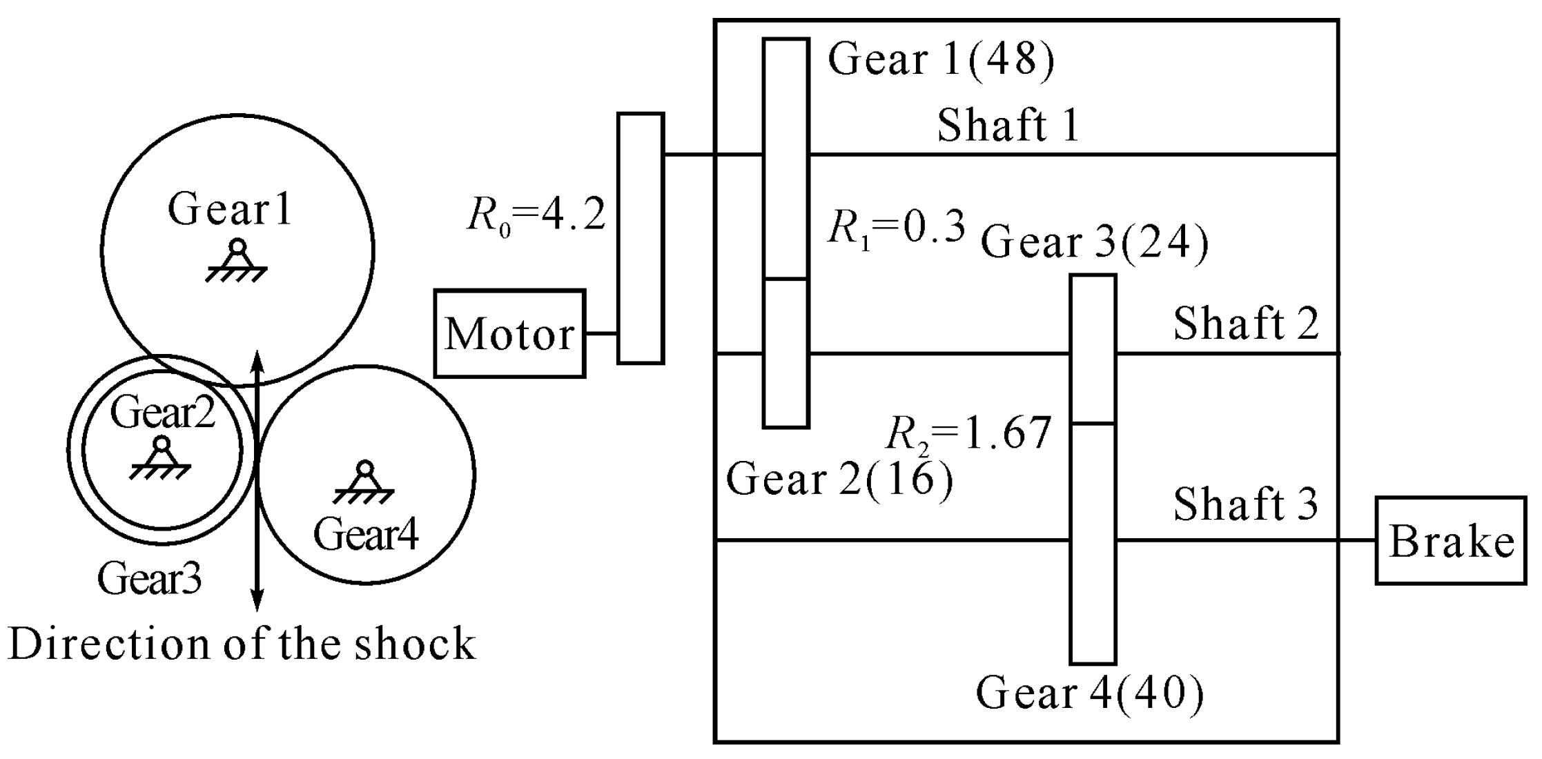
As shown in Figure 4, the dynamic acceleration of the gearbox system was excited by the vertical meshing mechanics of Gear 3 and Gear 4. Sensors placed vertically are more sensitive to this failure mode than sensors placed horizontally, and they can collect more comprehensive data of the outer cast of the gearbox. Gears 3 and 4 were chosen to simulate actual failure modes in industrial applications. It was difficult to determine which gear failed first. Based on existing experimental research, Gear 3 was chosen to simulate gear failure by cracking during the experimental procedure.

The experimental motor speed was chosen to be 2800 r/min, which caused the sampling frequency to be 12,800 Hz. Initial condition parameters, such as the safety factor (1.15) and the number of teeth in each gear, were set up. The angular velocities and characteristic frequencies of the shafts and gears inside the gearbox were calculated based on the drive ratio between the drive motor and the driven gears and the rotational speed of the drive motor. In

Table 2. Rotational parameters of the mechanical transmission.

Drive Motor (r/min)	Shaft Torque (N/m)	${\mathit{S}}_1$ (Hz)	${\mathit{G}}_{12}$ (Hz)	${\mathit{S}}_2$ (Hz)	${\mathit{G}}_{34}$ (Hz)	${\mathit{S}}_3$ (Hz)
2800.00	14.79	11.11	533.33	33.33	800	20

, $S_1$ indicates the speed of the first shaft that is mounted with the first gear, $S_2$ indicates the speed of the second shaft that is mounted with the second and third gears, $S_3$ indicates the speed of the third shaft that is mounted with the fourth gear, $G_{12}$ is the meshing frequency of the first and second gears, and $G_{34}$ is the meshing frequency of the third and fourth gears.

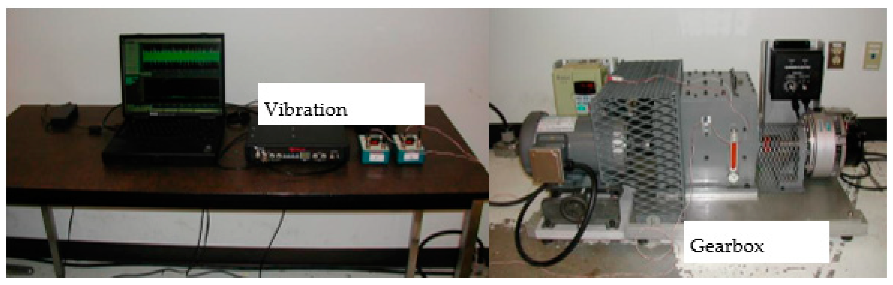
The vibration-signal acquisition system used for gearbox fault diagnosis in this study is displayed in Figure 5. Accelerometers (352C67-PCB) were installed on the gearbox cast. The vertical and horizontal components of the vibration signals were collected with a dynamic simulator (Spectra Quest). The vibration data were transmitted to a computer via a digital signal processor. The vibration signals of both data channels were synchronously acquired and analyzed using the proposed method.

4. Results and Discussion

4.1. Simulated Signal

The purpose of testing the numerical signals was to assess the capability of the proposed method, which was based on the parallel-factor analysis principle with signal processing, for fault-feature extraction. The simulated signal in Equation (18) was used to represent the fault modes of the gears in the gearbox because it is characteristic of the fault frequencies and impulses. The chosen fault modes were incipient cracks in the inner ring of the bearing. The simulated signal was defined according to the following:

$$\left\{\begin{array}{c}\mathrm{y}\left(\mathrm{t}\right)=\sum _{\mathrm{i}}{\mathrm{H}}_{\mathrm{k}}\mathrm{x}\left(\mathrm{t}-\mathrm{k}\mathrm{T}\right)\\ \mathrm{x}\left(\mathrm{t}\right)=\mathrm{e}\mathrm{x}\mathrm{p}\left(-\mathsf{\lambda }\mathrm{t}\right)\mathrm{c}\mathrm{o}\mathrm{s}\left(2\mathsf{\pi }{\mathrm{f}}_{\mathrm{n}}\mathrm{t}\right).\\ {\mathrm{H}}_{\mathrm{k}}=1+{\mathrm{H}}_0\mathrm{c}\mathrm{o}\mathrm{s}\left(2\mathsf{\pi }{\mathrm{f}}_{\mathrm{r}}\mathrm{t}\right)\end{array}\right.$$

(18)

In Equation (18), the function $\mathrm{y}\left(\mathrm{t}\right)$ is the periodic shock signal. The rotation frequency ${(\mathrm{f}}_{\mathrm{r}})$ was 20 Hz, while the intrinsic frequency $\left({\mathrm{f}}_{\mathrm{n}}\right)$ was 0.5 kHz. The frequency $\left({\mathrm{f}}_{\mathrm{s}}\right)$ of the accelerometer used for collecting vibration data was 1.6 kHz. There were 8192 data points within one vibration-signal group. The attenuation factor $\left(\mathsf{\lambda }\right)$ was 700, the displacement constant $\left({\mathrm{H}}_0\right)$ was 0.3, the repetition period (T) was 1/120, and the fault characteristic frequency ${(\mathrm{f}}_{\mathrm{i}})$ was 120 Hz.

Figure 6 depicts the time and frequency features of the characteristic impulse signal used to simulate the fault-feature information of the inner ring failure of the bearing. The basis wavelet function with “cmor3-3”, a complex Morlet wavelet, was used to transform the simulated signal into a 2D continuous wavelet factor matrix. A 1 × 200 × 8192 third-order tensor was constructed as the input to the PARAFAC model to obtain the loading values, the residual variance, and the normal distribution rate, which provided the channel, frequency, and time information, respectively.

Multi-scale parallel factorization with three-level decomposition was proposed to analyze the simulated signal. As shown in Figure 7, Mode 2 depicts the frequency-domain features under the three-level decomposition. The visible impulse signals of the simulated signal in Mode 2 had frequency peaks near 5000 Hz and in the 0–100 Hz range, which reflect the frequencies of the original signal shown in Figure 6. The characteristic low frequencies that indicate failure were not clearly extracted. The simulated signal from Equation (18) was used to test the proposed method. Figure 6 depicts the frequency components that are included in Equation (18). Figure 7 depicts the multi-level parallel factorization of the simulated signal, which exhibits the same frequency components and ranges as the original signal in Equation (18). The analog signals can therefore be used as a reference to verify the effectiveness of the proposed method.

The signal in Mode 3 shows the time-domain information after the multi-level decomposition with parallel factorization. Figure 8 shows the frequencies of the three component signals in Mode 3 after a Fourier transform was performed. There were frequency peaks at 20 Hz and 120 Hz, 240 Hz, and 360 Hz, which correspond to the rotational frequencies, the failure frequencies, and the harmonic frequencies, respectively. The developed parallel-factor algorithm was thus proven to be effective because it produced similar results as the traditional time–frequency domain signal-processing method for signal-feature extraction during mechanical fault diagnosis. The results show, however, that the proposed multi-scale parallel-factor algorithm is more accurate and efficient than the traditional time–frequency domain signal-processing methods.

4.2. PARAFAC–APSO–SVM Optimization

The vibration signal obtained from the gearbox was analyzed with the PARAFAC–APSO–SVM method. The rotational speed of the input rotor of the motor was chosen to be 2800 r/min. The five failure modes (F1, F2, F3, F4, and F5) represented different crack depths under no-load running conditions. The data group contained three sets of sampled signals for each mode. There were 8192 sampled data points in each vibration-signal set.

The vibration data acquired from the gearbox were processed by the PARAFAC model. The established PARAFAC model is sensitive to the number of factors. If the number of PARAFAC factors is estimated too high, the model error cannot be decreased, while if the number is too low, one valid solution cannot be obtained. In the present study, cross-validation was proposed to achieve an initial estimate of the number of PARAFAC factors while maintaining the accuracy of the PARAFAC multi-decomposition. The cross-validation process consisted of designating a portion of the data as missing and removing it, fitting the model to the remaining data, and then calculating the residuals between the fitted and actual missing data points. If the residual was too large, the model was considered to have poor performance. As shown in Figure 9, when there were more than four factors, the residual percentage of the cross-validation method was relatively low, which indicates that the residuals between the fitted data points and the actual missing data points were too large. This proves that an excessive number of PARAFAC factors can cause a decrease in cross-validation accuracy. Too few factors cannot yield an effective solution either. To ensure the highest cross-validation accuracy, the maximum number of factors was selected. The number of factors was set to fall within the range of one to seven for the cross-validation. The figure shows that the variation percentages in the fit and the cross-validation were much better, equal to 86.7% and 85.3%, respectively, when there were four factors.

Kernel consistency estimation is another effective method of calculating the number of factors. It is based on the principle that the number of factors can be calculated by assessing the similarity between the super-diagonal matrix and the core 3D data matrix within the constructed parallel-factor model. This method was chosen to validate the number of factors determined by cross-validation during this study.

Kernel consistency estimation was proposed by Bro et al. [17] and its feasibility has been widely recognized. This method determines an initial estimated value by calculating the similarity between the super-diagonal matrix (T) in the model and the core 3D data matrix (G). The kernel consistency ($\delta$) is defined according to Equation (19):

$$\mathsf{\delta }=100\times \left(1-\frac{{\displaystyle \sum _{\mathrm{d}=1}^{\mathrm{F}}{\displaystyle \sum _{\mathrm{e}=1}^{\mathrm{F}}{\displaystyle \sum _{\mathrm{f}=1}^{\mathrm{F}}{({{\displaystyle \mathrm{g}}}_{\mathrm{d}\mathrm{e}\mathrm{f}}-{{\displaystyle \mathrm{t}}}_{\mathrm{d}\mathrm{e}\mathrm{f}})}^2}}}}{\mathrm{F}}\right),$$

(19)

where ${\mathrm{g}}_{\mathrm{d}\mathrm{e}\mathrm{f}}$ represents an element in matrix G, ${\mathrm{t}}_{\mathrm{d}\mathrm{e}\mathrm{f}}$ is an element in matrix T, and F is the number of factors. In the ideal PARAFAC model, the similarity between T and G reaches 100%. In general, if the kernel consistency value is greater than or equal to 60%, the PARAFAC model is considered to be trilinear. If the kernel consistency value is less than 60%, the PARAFAC model is considered to have deviated from the trilinear. A more accurate estimate of the F-value can be obtained from its variation pattern.

Figure 10 shows the results of the kernel consistency test. The yellow line represents the target value. The red points are non-zero data points, and the blue points are zero data points, which were within the basic agreement range with respect to the target curve. The consistency rate was approximately 100%.

4.3. Feature Extraction with the PARAFAC Data

The vibration signals collected in the normal and fault modes were processed. The continuous wavelet transform, with the wavelet basis function “cmor3-3”, was used to extract the time- and frequency-domain information from the vibration signals. As explained in Section 4.1, the analysis of the simulated signal verified that the data had higher resolution under the frequency and time loading models; thus, the normal and fault information, which was obtained using parallel-factor decomposition, could be characterized for the three models. The information for the two mode types was extracted from the binary conditions, that is, the normal and fault conditions. Figure 11 and Figure 12 show the vibration signal analysis performed with PARAFAC multi-decomposition under normal and fault conditions. There were four components for the time loading and the frequency loading. Eight features were calculated for the PARAFAC factors of Modes 2 and 3; these included the mean value, the root mean square value, the root mean, the center of gravity frequency, the root mean square frequency, the standard deviation, the cliff value, and the skewness, which are defined in Equations (20)–(27). One set of feature vectors consisted of 64 parameters.

$$\stackrel{-}{\mathrm{x}}=\frac{1}{\mathrm{A}}{\sum }_{\mathrm{a}=1}^{\mathrm{A}}\mathrm{x}\left(\mathrm{a}\right),$$

(20)

$${\mathrm{x}}_{\mathrm{r}}={\left(\frac{1}{\mathrm{A}}{\sum }_{\mathrm{a}=1}^{\mathrm{A}}\sqrt{\left|\mathrm{x}\left(\mathrm{a}\right)\right|}\right)}^2,$$

(21)

$${\mathrm{x}}_{\mathrm{r}\mathrm{m}\mathrm{s}}=\sqrt{\frac{1}{\mathrm{A}}{\sum }_{\mathrm{a}=1}^{\mathrm{A}}{\mathrm{x}}^2\left(\mathrm{a}\right)},$$

(22)

$${\mathrm{F}}_{\mathrm{c}}=\frac{{\sum }_{\mathrm{a}=1}^{\mathrm{A}}{\mathrm{f}}_{\mathrm{A}}·\mathrm{x}\left(\mathrm{a}\right)}{{\sum }_{\mathrm{a}=1}^{\mathrm{A}}\mathrm{x}\left(\mathrm{a}\right)},$$

(23)

$${\mathrm{F}}_{\mathrm{r}\mathrm{m}\mathrm{s}}=\frac{{\sum }_{\mathrm{a}=1}^{\mathrm{A}}{\mathrm{f}}_{\mathrm{A}}·\mathrm{x}\left(\mathrm{a}\right)}{{\sum }_{\mathrm{a}=1}^{\mathrm{A}}\mathrm{x}\left(\mathrm{a}\right)},$$

(24)

$${\mathsf{\sigma }}_{\mathrm{x}}=\sqrt{\frac{1}{\mathrm{A}-1}{\sum }_{\mathrm{a}=1}^{\mathrm{A}}{\left[\mathrm{x}\left(\mathrm{a}\right)-\stackrel{-}{\mathrm{x}}\right]}^2},$$

(25)

$$\mathrm{K}=\frac{{\sum }_{\mathrm{a}=1}^{\mathrm{A}}{\left[\mathrm{x}\left(\mathrm{a}\right)-\stackrel{-}{\mathrm{x}}\right]}^4}{\left(\mathrm{A}-1\right){{\mathsf{\sigma }}_{\mathrm{x}}}^4},$$

(26)

$$\mathrm{S}=\frac{{\sum }_{\mathrm{a}=1}^{\mathrm{A}}{\left[\mathrm{x}\left(\mathrm{a}\right)-\stackrel{-}{\mathrm{x}}\right]}^3}{\left(\mathrm{A}-1\right){{\mathsf{\sigma }}_{\mathrm{x}}}^3}.$$

(27)

4.4. Fault Diagnosis Based on the APSO–SVMPSO–SVM Model

There were 160 sets of feature vectors for one gearbox mode. The total number of vector sets for the normal mode and the four fault modes was 800. Seven hundred groups of vibration signals were considered to be training data and the other one hundred groups were the testing input features for the SVM classifier and the optimized APSO–SVM model. The parameters set for the PSO algorithm included a particle swarm size of 20, 200 iterations, an acceleration factor (C1) of 1.5, and an acceleration factor (C2) of 1.7. Figure 13 presents a comparison between the true values and the values predicted by the SVM classifier. Figure 14 depicts a comparison between the true values and the values predicted by the APSO–SVM model. The classification correction rate of the SVM model was 93% and the classification correction rate of the optimized APSO–SVM model was 98%. The APSO–SVM model had significant advantages over the SVM classifier because of the optimized SVM variables.

Table 3. Comparison between the four types of classifiers.

Classifier	Correction Rate	Running Time (s)
CWT–SVM	72%	2.624
S–PARAFAC–SVM	90%	2.437
D–PARAFAC–SVM	93%	3.151
D–PARAFAC–APSO–SVM	98%	16.593

shows a comparison between the correction rates of the four classifiers, which was used to test the differences between their fault-condition classification capabilities. The CWT–SVM classifier model used the wavelet packet energy of the vibration signals within a single channel as the input feature vectors for the SVM. The S–PARAFAC–SVM model used the parallel factors of the vibration signals within a single channel as the input feature vectors for the SVM. The D-PARAFAC-SVM used the parallel factors of a dual-channel vibration signal analysis as the input feature vectors for the SVM. The D–PARAFAC–APSO–SVM model used the parallel-factors of a dual-channel vibration signal analysis as the input feature vectors for the SVM with APSO optimization.

As shown in Table 3, the correction rate and running time of the CWT–SVM classifier were 72% and 2.624 s, respectively. The correction rate and running time of the S–PARAFAC–SVM classifier were 90% and 2.437 s, respectively, which represented significant improvements over the CWT–SVM results. The correction rate and running time of the D–PARAFAC–SVM classifier were 93% and 3.151 s, respectively. The D–PARAFAC–SVM classifier had a much better correction rate than the S–PARAFAC–SVM classifier, which indicates that dual-channel PARAFAC data analysis is superior to single-channel PARAFAC vibration signal analysis. The D–PARAFAC–APSO–SVM classifier had a 98% correction rate, which was the highest correction rate of the four classifiers. Therefore, it was verified that dual-channel PARAFAC data analysis had a significantly improved classification capability when it was combined with the advantages of APSO optimization for an SVM.

5. Conclusions

In this study, the parallel-factor multi-level decomposition theory was investigated with the goal of proposing a hybrid method for multi-channel, multi-scale data mining. Compared to traditional dimensionality reduction methods, parallel factor models retain more signal fault information, thereby improving the accuracy of fault feature extraction.

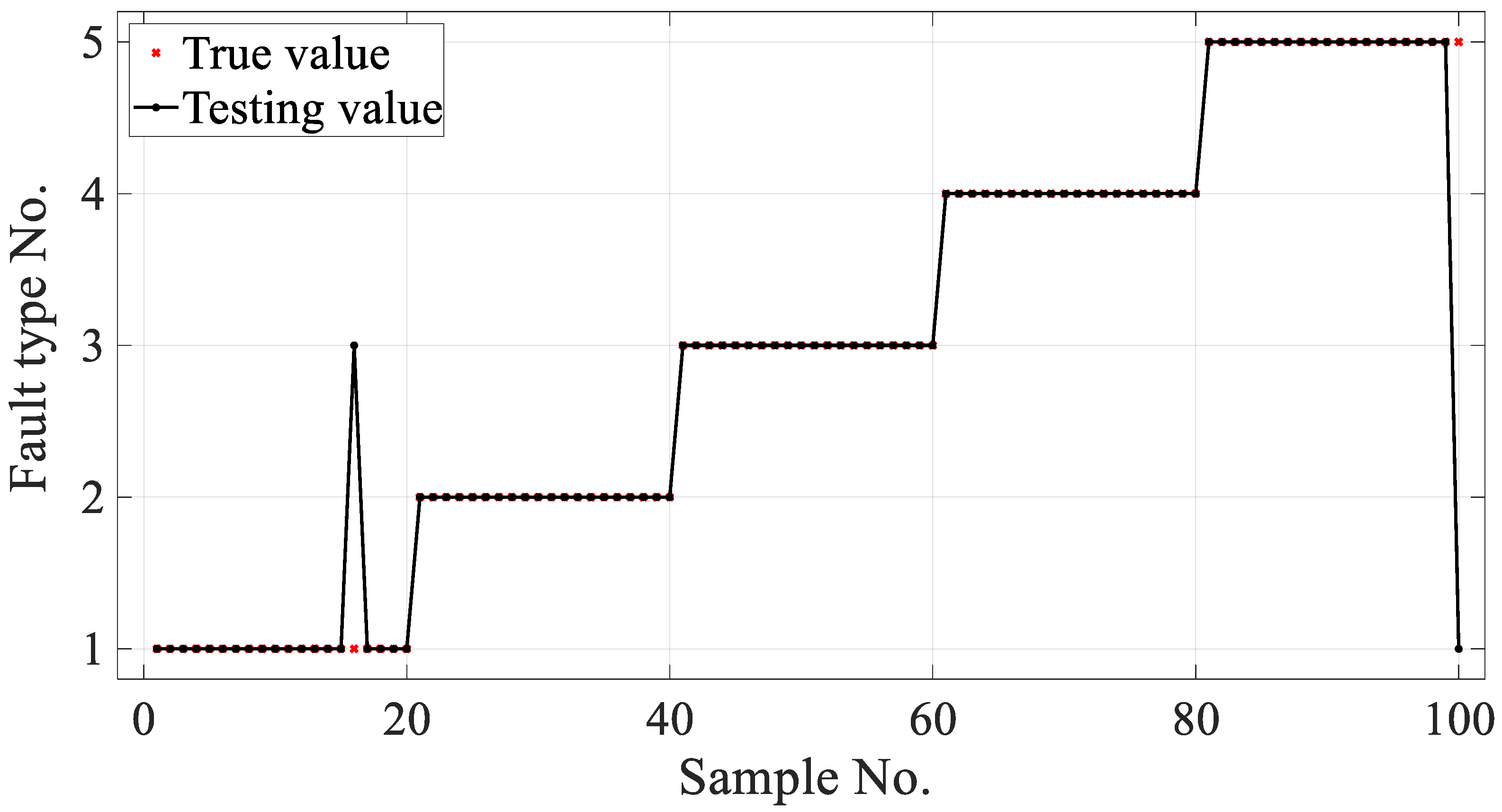
A larger classification correction rate for the condition monitoring of gear failures in a gearbox was achieved by using the developed PARAFAC–APSO–SVM classifier. The parameters of a traditional SVM were optimized using APSO to improve the recognition of different gearbox failure modes. In future work, it will be necessary to improve the reliability and robustness of the classifier for use in complex industrial applications.