Kinematics and Dynamics Analysis of a 3UPS-UPU-S Parallel Mechanism

Abstract

In this paper, a two-rotational degrees of freedom parallel mechanism with five kinematic subchains (3UPS-UPU-S) (U, P, and S stand for universal joints, prismatic joints, and spherical joints) for an aerospace product is introduced, and its kinematic and dynamic characteristics are subsequently analyzed. The kinematic and dynamic analyses of this mechanism are carried out in screw coordinates. Firstly, the inverse kinematics is performed through the kinematic equations established by the velocity screws of each joint to obtain the position, posture, and velocity of each joint within the mechanism. Then, a dynamic modeling method with screw theory for multi-body systems is proposed. In this method, the momentum screws are established by the momentum and moment of momentum according to the fundamentals of screws. By using the kinematic parameters of joints, the dynamic analysis can be carried out through the dynamic equations formed by momentum screws and force screws. This method unifies the kinematic and dynamic analyses by expressing all parameters in screw form. The approach can be employed in the development of computational dynamics because of its simplified and straightforward analysis procedure and its high adaptability for different kinds of multi-body systems.

1. Introduction

Multi-body systems offer multiple advantages over single-body systems, including improved load distribution, enhanced flexibility, and increased adaptability to diverse operating conditions. These systems find extensive applications in various fields, such as robotics, aerospace, automotive, and manufacturing industries. Among them, parallel mechanisms have garnered significant attention due to their high rigidity, accuracy, and ability to perform precise, complex motion tasks. Despite their inherent complexity and non-linearity, redundantly actuated parallel mechanisms are extensively designed to overcome singularity issues and enhance structural stiffness and load capacity.

Understanding the kinematics and dynamics of parallel platforms is crucial for their practical implementation. Kinematic analysis reveals the motion characteristics of parallel mechanisms by solving the kinematic parameters such as posture, position, and velocity of individual joints within the system. By using conventional kinematic modeling approaches to describe both rotational and translational motions, a suitable mathematical framework in a relatively general way is required. Screw coordinates have been proposed as a valuable tool to simplify the kinematic analysis of parallel mechanisms [1].

Dynamics analysis plays a significant role in achieving robot control, motion stability, and structural optimization. However, redundantly actuated parallel mechanisms present challenges in dynamic modeling due to their complexity and computational requirements. Several methods have been proposed to analyze the dynamics of multi-rigid-body systems, including Lagrange equations [2,3], Newton–Euler equations [4,5,6], virtual work principles [7,8,9,10], Kane equations [11,12], and Gibbs–Appell equations [13,14]. The analysis of multi-rigid-body systems often relies on mathematical methods from classical mechanics and vector equations [7,15]. Additionally, the screw theory has been extensively used for dynamic analysis, providing efficient modeling of mechanisms based on kinematic formulations through screw theory [16,17,18]. As Pennock has discussed the geometric relationship between velocity screws and momentum screws [19], researchers such as Gallardo [17,20] have presented kinematic and dynamic models for parallel mechanisms utilizing screw coordinates. Müller has pointed out that besides the contribution to the kinematic analysis made by screw theory, screw theory and the Lie group can also be applied to the dynamic analysis of multi-body systems with high efficiency [21,22]. Zhao [5] has investigated an approach to dynamic analysis of multi-body systems by expressing acceleration in screw form using screw and Lie products, but the dynamic equations are established using the velocity expressed in screw coordinates as a global variable according to the Newton–Euler method. Dynamic analysis is rarely carried out systematically by screw theory. Therefore, this paper focuses on dynamic modeling by combining momentum screws and force screws. And a novel procedure to obtain dynamic equations through differential equations based on the theorem of the momentum screw is proposed and applied to the dynamics of various mechanisms.

In this paper, we present the design of a parallel mechanism with five kinematic chains to achieve two rotational degrees of freedom (DoFs) according to the task demands and propose a novel dynamic modeling process by establishing the dynamic equations derived from the theorem of momentum to simplify the dynamic analysis in a concise manner.

The main contributions of this paper are as follows:

(1)

The dynamic equations of the differential momentum screw and force screw are deduced in detail. There is no acceleration needed in dynamic modeling. It shows that utilizing momentum and the moment of momentum screws offers a clearer physical interpretation of the dynamics analysis and facilitates computation in programming.

(2)

The forces and torques of each joint can be simultaneously solved in the absolute coordinate system.

(3)

The programming code of this algorithm is compact and easy to structure and debug. This method can be applied not only to the analysis of parallel mechanisms but also to planar and spatial mechanisms.

2. Geometry Design of the Parallel Mechanism

A parallel mechanism incorporating five kinematic subchains has been designed to fill a task demand with two rotational DoFs, and the overall size, occupation of the parts within the mechanism, some designated structure, and other factors have been considered. Five kinematic subchains are assembled and connect the base and the moving platform to achieve continuous swiveling on two axes, and the DoFs are computed and verified in Section 3.2. As illustrated in Figure 1, this parallel platform consists of a base and a mobile platform, which is formed with a spherical joint to obtain a kinematic chain denoted as {S}. Additionally, the mechanism consists of three kinematic chains denoted as {UPS} and one kinematic chain denoted as {UPU}, where the letters U, P, and S signify universal joint, prismatic pair, and spherical joint, respectively. The primary U joints of four side kinematic chains are distributed and assembled uniformly along the edge of the base at points $A_1$, $A_2$, $A_3$, and $A_4$, while four last joints including one U joint and three S joints are assembled on the edge of moving platform at points $C_1$, $C_2$, $C_3$, and $C_4$. The radii of circumcircle of $A_1{A}_2{A}_3{A}_4$ and $C_1{C}_2{C}_3{C}_4$ are $R$ and $r$, respectively. The fifth kinematic chain {S} has only one spherical joint, its revolute center is coincided with the geometrical center of the base, and here is the origin of the coordinate system: $O$. The first rotary aches of the primary U joints in chains {UPU} and {UPS} fixed on the base are coplanar and intersect at the origin $O$. On the initial assembly configuration, the universal joint planes of all universal joints and the moving platform plane are parallel to the base plane.

As the origin $O$ is chosen at the geometrical center of the base, and the $z$-axis is perpendicular to the base and points to the moving platform, the $x$-axis points to $A_3$, then, the $y$-axis can be settled through right-hand rule.

3. Kinematics Analysis

3.1. Fundamentals of Screw Theory

To describe the rotational motion of a free rigid body in the reference coordinate frame, the angular velocity $\mathit{\omega }$ can be expressed through:

$$\mathit{\omega }={\omega }_1{\mathit{e}}_1+{\omega }_2{\mathit{e}}_2+{\omega }_3{\mathit{e}}_3$$

(1)

where ${\mathit{e}}_1, {\mathit{e}}_2, {\mathit{e}}_3$ are unit direction vectors and ${\omega }_1, {\omega }_2, {\omega }_3$ are the amplitude of the components of $\mathit{\omega }$ in ${\mathit{e}}_1, {\mathit{e}}_2, {\mathit{e}}_3$. Therefore, the expression of angular velocity of the free rigid body can be simplified as

$$\mathit{\omega }={\left[\begin{array}{ccc}{\omega }_1& {\omega }_2& {\omega }_3\end{array}\right]}^{\mathrm{T}}$$

(2)

Then, with $\mathit{r}=x{\mathit{e}}_1+y{\mathit{e}}_2+z{\mathit{e}}_3$ presenting the position vector of the point attached on this rigid body, the linear velocity of this point passing through the origin is

$$\mathit{v}=\frac{\mathrm{d}\mathit{r}}{\mathrm{d}\mathit{t}}=\mathit{\omega }\times \mathit{r}$$

(3)

The kinematics of a joint in a serial kinematic chain are relative to the kinematics of the fore joints. Based on the addition theorem for angular velocities, the angular velocity and the linear velocity of joint $J_m$ in a serial kinematic chain with respect to the absolute coordinate frame $O$ can be obtained as follows:

$$\{\begin{array}{l}{}_O{}^m\mathit{\omega }={}_O{}^1\mathit{\omega }+{}_1{}^2\mathit{\omega }+{}_2{}^3\mathit{\omega }+\cdots +{}_{m-2}{}^{m-1}\mathit{\omega }+{}_{m-1}{}^m\mathit{\omega }\\ {}_O{}^m\mathit{v}=\frac{\mathrm{d}{}_O{}^m\mathit{r}}{\mathrm{d}t}={}_O{}^m\mathit{\omega }\times \mathit{r}\end{array}$$

(4)

According to the screw theory, the velocity of joint $J_m$ can be specified by dual 3-dimensional vectors ${}_O{}^m\mathit{\omega }$ and ${}_O{}^m\mathit{v}$. Therefore, in the following, the relative velocity screw ${}_{m-1}^m{\cancel{\mathit{S}}}_V$ of joint $J_m$ in screw coordinate is defined as:

$${}_{m-1}{}^m\cancel{\mathit{S}}{}_V=\left[\begin{array}{c}{}_{m-1}{}^m\mathit{\omega }\\ {}_0{}^m\mathit{r}\times {}_{m-1}{}^m\mathit{\omega }\end{array}\right]={}_{m-1}{}^m\omega \left[\begin{array}{c}{}_{m-1}{}^m\mathit{e}\\ {}_0{}^m\mathit{r}\times {}_{m-1}{}^m\mathit{e}\end{array}\right]={}_{m-1}{}^m\omega {}_{m-1}{}^m\cancel{\mathit{S}}{}_u$$

(5)

where ${}_{m-1}{}^m\omega$ is the magnitude of the relative angular velocity of joint $J_m$ with respect to joint $J_{m-1}$ and the unit vector along the rotary axis is ${\mathit{e}}_m$, which norm is $\Vert {\mathit{e}}_m\Vert =1$, ${}_{m-1}{}^m\cancel{\mathit{S}}{}_u$ represents the unit relative velocity screw of joint $J_m$.

From Equations (4) and (5), the forward kinematics of the kinematic chain having $n$ joints in serial can be derived through:

$${}_0^n{\cancel{\mathit{S}}}_V={\displaystyle \sum _{i=1}^n{}_{i-1}^i{\cancel{\mathit{S}}}_V}={\mathbf{S}}_V{\mathit{\omega }}_V$$

(6)

where ${\mathbf{S}}_V={\left[\begin{array}{cccc}{}_0^1{\cancel{\mathit{S}}}_u& {}_1^2{\cancel{\mathit{S}}}_u& \cdots & {}_{n-1}^n{\cancel{\mathit{S}}}_u\end{array}\right]}_{6\times n}$ represents the unit velocity screw matrix of a serial chain with $n$ joints and ${\mathit{\omega }}_V={\left[\begin{array}{cccc}{}_0^1\omega & {}_1^2\omega & \cdots & {}_{n-1}^n\omega \end{array}\right]}_{n\times 1}^{\mathrm{T}}$ expressing the angular velocity vector containing all relative angular velocities of every joint in this chain relative to its fore joint, with $0$ referring to the origin of the coordinate frame.

On the other hand, when the kinematics of the end effector in the absolute coordinate frame are known, the angular velocity vector can be solved by

$${\mathit{\omega }}_V={\left[{\mathbf{S}}_V^{\mathrm{T}}{\mathbf{S}}_V\right]}^{-1}{\mathbf{S}}_V^{\mathrm{T}}\left({}_0^n{\cancel{\mathit{S}}}_V\right)$$

(7)

If the mechanism is neither redundantly actuated nor in a singularity configuration, it meets $\left|{\mathbf{S}}_V^{\mathrm{T}}{\mathbf{S}}_V\right|\ne 0$. ${\left[{\mathbf{S}}_V^{\mathrm{T}}{\mathbf{S}}_V\right]}^{-1}{\mathbf{S}}_V^{\mathrm{T}}$ is called the pseudo-inverse of the unit velocity screw matrix ${\mathbf{S}}_V$. Through the velocity parameters from Equation (7), the displacement and acceleration can be gained by first-order numerical integration and first-order numerical differential interpolation, respectively.

During verse kinematics analysis process, at $t=0$, the initial conditions of the angular displacement vector $\mathit{\theta }(0)$ is given in form:

$$\mathit{\theta }(0)={\left[\begin{array}{cccc}\begin{array}{cc}{}_0^1\theta (0)& {}_1^2\theta (0)\end{array}& \cdots & {}_{n-2}^{n-1}\theta (0)& {}_{n-1}^n\theta (0)\end{array}\right]}_{n\times 1}^{\mathrm{T}}$$

(8)

Equation (8) is then substituted into unit screw matrix ${\mathbf{S}}_V$ in Equation (5) to calculate the solution of ${\mathit{\omega }}_V\left(1\right)$ for the first-time segment. Afterwards, the successive parameters of ${\mathbf{S}}_V\left(k\right)$ at $t=k\Delta t$ can be updated by:

$$\mathit{\theta }\left(k+1\right)=\mathit{\theta }\left(k\right)+\Delta t{\mathit{\omega }}_{\mathrm{V}}\left(k\right)$$

(9)

with $k=1,2,\cdots$ presenting the steps of iteration.

Within the ${\mathbf{S}}_V\left(k\right)$, the position vector ${}_0{}^m\mathit{r}$ and posture ${}_{m-1}{}^m\mathit{e}$ of $m$-th joints with $m=1,2,\cdots ,n$ can be obtained.

3.2. Workspace and Mobility Analysis of the $3UPS-UPU-S$ Parallel Mechanism

This parallel mechanism is designed based on a specified application. It is required to have two rotational degrees of freedom around the $x$- and $y$-axis as shown in Figure 1. The demanded swing angles of the moving platform, as illustrated in Figure 2 are 10°. As universal joints and spherical joints in kinematic chains have only a little effect on the workspace regarding the designated swing angles, the workspace is limited mainly by the effective length of subchains with the prismatic joints. The design of the chain length and the selection of prismatic joints are determined by the required swing angles.

Figure 3 depicts the unit vector of all kinematic joints in each chain. As the velocities, positions, and postures of each joint are expressed in screw coordinates, the reciprocal screw theory is employed here to compute the mobility of this parallel mechanism. In accordance with the reciprocal screw theory, there is:

$${\mathbf{S}}_V^{\mathrm{T}}\aleph {\cancel{\mathit{S}}}^r=0$$

(10)

where $\mathbf{\aleph }=\left[\begin{array}{cc}0& {\mathit{I}}_{3\times 3}\\ {\mathit{I}}_{3\times 3}& 0\end{array}\right]$ and the 3rd-order identity matrix ${\mathit{I}}_{3\times 3}=\left[\begin{array}{ccc}1& 0& 0\\ 0& 1& 0\\ 0& 0& 1\end{array}\right]$.

The kinematic screws of the 1st subchain {UPU} can be expressed by five joints as:

$$\begin{array}{l}{\cancel{\mathit{S}}}_{UPU}^1={\left[\begin{array}{cccccc}1& 0& 0& 0& 0& 0\end{array}\right]}^{\mathrm{T}}\\ {\cancel{\mathit{S}}}_{UPU}^2={\left[\begin{array}{cccccc}0& 1& 0& 0& 0& -R\end{array}\right]}^{\mathrm{T}}\\ {\cancel{\mathit{S}}}_{UPU}^3={\left[\begin{array}{cccccc}0& 0& 0& \sin \theta & 0& \cos \theta \end{array}\right]}^{\mathrm{T}}\\ {\cancel{\mathit{S}}}_{UPU}^4={\left[\begin{array}{cccccc}\cos \theta & 0& -\sin \theta & 0& R\sin \theta -L& 0\end{array}\right]}^{\mathrm{T}}\\ {\cancel{\mathit{S}}}_{UPU}^5={\left[\begin{array}{cccccc}0& 1& 0& L\cos \theta & 0& R-L\sin \theta \end{array}\right]}^{\mathrm{T}}\end{array}$$

(11)

where $L_{UPU}$ is the total length of the {UPU} chain and $\theta$ represents the angle between {UPU} chain and $z$-axis.

From Equation (11), the screw matrix of {UPU} chain can be obtained:

$${\mathbf{S}}_1=\left[\begin{array}{ccccc}{\cancel{\mathit{S}}}_{UPU}^1& {\cancel{\mathit{S}}}_{UPU}^2& {\cancel{\mathit{S}}}_{UPU}^3& {\cancel{\mathit{S}}}_{UPU}^4& {\cancel{\mathit{S}}}_{UPU}^5\end{array}\right]$$

(12)

Therefore, the inverse screw of {UPU} chain can be derived based on Equation (12):

$${\cancel{\mathit{S}}}_{UPU}^r={\left[\begin{array}{cccccc}0& 1& 0& 0& 0& -R+\frac{L}{\sin \theta }\end{array}\right]}^{\mathrm{T}}$$

(13)

Through the definition of a screw, Equation (13) denotes a force parallel to $y$-axis and passing through point $\left(\begin{array}{ccc}-R+\frac{L}{\sin \theta }& y& 0\end{array}\right)$, where $y$ can be any significant real number.

Similarly, the inverse screws of three {UPS} chains and {S} chain can be obtained as:

$${\cancel{\mathit{S}}}_{UPS}^r={\left[\begin{array}{cccccc}0& 0& 0& 0& 0& 0\end{array}\right]}^{\mathrm{T}}$$

(14)

and

$${\cancel{\mathit{S}}}_S^r={\left[\begin{array}{cccccc}1& 0& 0& 0& 0& 0\\ 0& 1& 0& 0& 0& 0\\ 0& 0& 1& 0& 0& 0\end{array}\right]}^{\mathrm{T}}$$

(15)

From Equations (13)–(15), the terminal constraints of the moving platform can be obtained as

$${\mathbf{S}}_P^C=\left[\begin{array}{cccc}0& 1& 0& 0\\ 1& 0& 1& 0\\ 0& 0& 0& 1\\ 0& 0& 0& 0\\ 0& 0& 0& 0\\ -R+\frac{L}{\sin \theta }& 0& 0& 0\end{array}\right]$$

(16)

The free velocity screws of the moving platform can also be computed from the reciprocal screw method, which is:

$${\left({\mathbf{S}}_P^C\right)}^{\mathrm{T}}\mathbf{\aleph }{\cancel{\mathit{S}}}_P=0$$

(17)

Therefore, the mobility of this parallel mechanism can be derived as

$${\cancel{\mathit{S}}}_P={\left[\begin{array}{cccccc}1& 0& 0& 0& 0& 0\\ 0& 1& 0& 0& 0& 0\end{array}\right]}^{\mathrm{T}}$$

(18)

Equation (19) indicates that the mechanism has two rotational degrees of freedom around $x$- and $y$-axis of the coordinate frame illustrated in Figure 2. From the calculation above, it can be seen that with one {UPU} chain, one {UPS} chain, and one {S} can also satisfy the mobility requirements. The two additional {UPS} subchains are designed to achieve better load distribution and stability.

3.3. Kinematic Modeling of the $3UPS-UPU-S$ Parallel Mechanism

Through the fundamentals of screws, the velocity screw matrix of each serial kinematic subchain could be obtained through Equations (5) and (6).

As shown in Figure 2, the velocity screw matrix of the 1st {UPU} chain can be expressed as:

$${\mathbf{S}}_V^1={\left[\begin{array}{ccccc}\begin{array}{c}{}_1{\mathit{e}}_1\\ {\mathit{r}}_{A1}{\times }_1{\mathit{e}}_1\end{array}& \begin{array}{c}{}_1{\mathit{e}}_2\\ {\mathit{r}}_{A1}{\times }_1{\mathit{e}}_2\end{array}& \begin{array}{c}\mathbf{0}\\ {}_1{\mathit{e}}_3\end{array}& \begin{array}{c}{}_1{\mathit{e}}_4\\ {\mathit{r}}_{C1}{\times }_1{\mathit{e}}_4\end{array}& \begin{array}{c}{}_1{\mathit{e}}_5\\ {\mathit{r}}_{C1}{\times }_1{\mathit{e}}_5\end{array}\end{array}\right]}_{6\times 5}$$

(19)

where ${}_1{\cancel{\mathit{S}}}_1=\left[\begin{array}{c}{}_1{\mathit{e}}_1\\ {}_1{\mathit{r}}_{U1}{\times }_1{\mathit{e}}_1\end{array}\right]$ is the unit velocity screw of a revolute joint and ${}_1{\cancel{\mathit{S}}}_3=\left[\begin{array}{c}\mathbf{0}\\ {}_1{\mathit{e}}_3\end{array}\right]$ denotes the unit velocity screw of a prismatic pair, and the subscript $6\times 5$ of the matrix represents the dimensions of the matrix.

Through the same procedure, the velocity screw matrix of 2nd to 4th {UPS} chains and 5th {S} chain can be gained as

$$\begin{array}{l}{\mathbf{S}}_V^i={\left[\begin{array}{cccccc}\begin{array}{c}{}_i{\mathit{e}}_1\\ {\mathit{r}}_{Ai}{\times }_i{\mathit{e}}_1\end{array}& \begin{array}{c}{}_i{\mathit{e}}_2\\ {\mathit{r}}_{Ai}{\times }_i{\mathit{e}}_2\end{array}& \begin{array}{c}\mathbf{0}\\ {}_i{\mathit{e}}_3\end{array}& \begin{array}{c}{}_i{\mathit{e}}_4\\ {\mathit{r}}_{Ci}{\times }_1{\mathit{e}}_4\end{array}& \begin{array}{c}{}_i{\mathit{e}}_5\\ {\mathit{r}}_{Ci}{\times }_1{\mathit{e}}_5\end{array}& \begin{array}{c}{}_i{\mathit{e}}_6\\ {\mathit{r}}_{Ci}{\times }_1{\mathit{e}}_5\end{array}\end{array}\right]}_{6\times 6}, i=2, 3, 4\\ {\mathbf{S}}_V^5={\left[\begin{array}{ccc}\begin{array}{c}{}_5{\mathit{e}}_1\\ {\mathit{r}}_{A5}{\times }_5{\mathit{e}}_1\end{array}& \begin{array}{c}{}_5{\mathit{e}}_2\\ {\mathit{r}}_{A5}{\times }_5{\mathit{e}}_2\end{array}& \begin{array}{c}{}_5{\mathit{e}}_3\\ {\mathit{r}}_{A5}{\times }_5{\mathit{e}}_3\end{array}\end{array}\right]}_{6\times 3}\end{array}$$

(20)

The kinematic screw equation of parallel mechanisms with multi kinematic chains can be written as:

$$\mathbf{S}\mathit{\omega }={\cancel{\mathit{S}}}_V$$

(21)

where

$$\mathbf{S}=\mathrm{diag}{\left[\begin{array}{ccccc}{\left[{\mathbf{S}}_V^1\right]}_{6\times 5}& {\left[{\mathbf{S}}_V^2\right]}_{6\times 6}& {\left[{\mathbf{S}}_V^3\right]}_{6\times 6}& {\left[{\mathbf{S}}_V^4\right]}_{6\times 6}& {\left[{\mathbf{S}}_V^5\right]}_{6\times 3}\end{array}\right]}_{30\times 26}$$

(22)

is composed of the velocity screw matrix of each kinematic chain and $\mathrm{diag}\left[\right]$ is the diagonal matrix of ${\mathbf{S}}_V^i \left(i=1,2,\cdots ,5\right)$, and

$$\mathit{\omega }={\left[\begin{array}{cccc}{\left[{\mathit{\omega }}^1\right]}_{5\times 1}^{\mathrm{T}}& {\left[{\mathit{\omega }}^2\right]}_{6\times 1}^{\mathrm{T}}& \cdots & {\left[{\mathit{\omega }}^5\right]}_{3\times 1}^{\mathrm{T}}\end{array}\right]}_{26\times 1}^{\mathrm{T}}$$

(23)

is the velocity vector and contains all the relative angular velocities of each kinematic joint.

The velocity screw ${\cancel{\mathit{S}}}_V$ can be expressed through

$${\cancel{\mathit{S}}}_V={\left[\begin{array}{ccccc}{\left[{}_O^{C_1}{\cancel{\mathit{S}}}_V^1\right]}_{6\times 1}^{\mathrm{T}}& {\left[{}_O^{C_2}{\cancel{\mathit{S}}}_V^2\right]}_{6\times 1}^{\mathrm{T}}& {\left[{}_O^{C_3}{\cancel{\mathit{S}}}_V^3\right]}_{6\times 1}^{\mathrm{T}}& {\left[{}_O^{C_4}{\cancel{\mathit{S}}}_V^4\right]}_{6\times 1}^{\mathrm{T}}& {\left[{}_O^{C_5}{\cancel{\mathit{S}}}_V^5\right]}_{6\times 1}^{\mathrm{T}}\end{array}\right]}_{30\times 1}^{\mathrm{T}}$$

(24)

with ${}_O^{C_i}{\cancel{\mathit{S}}}_V^i\left(i=1,2,\cdots ,5\right)$ representing the absolute velocity screws of the end effectors of $i$-th kinematic chain.

As the topological diagram illustrated in Figure 4, according to the given motion of the geometric center E on the outer ring of the moving platform ${}_O^E{\cancel{\mathit{S}}}_V$, the velocity screws of the end effectors of each kinematic chain ${}_O^{C_i}{\cancel{\mathit{S}}}_V^i\left(i=1,2,\cdots ,5\right)$ can be calculated by:

$${}_O^{C_i}{\cancel{\mathit{S}}}_V^i{=}_O^E{\cancel{\mathit{S}}}_V{-}_{C_i}^E{\cancel{\mathit{S}}}_V^i\left(i=1,2,\cdots ,5\right)$$

(25)

where ${}_{C_i}^E{\cancel{\mathit{S}}}_V^i\left(i=1,2,\cdots ,5\right)$ denotes the relative velocity screw of point E with respect to $C_i \left(i=1,2,\cdots ,5\right)$, which is

$${}_{C_i}^E{\cancel{\mathit{S}}}_V^i={\left[\begin{array}{c}\mathbf{0}\\ {}_O^{C_i}{\mathit{\omega }}^i\times {\mathit{r}}_E\end{array}\right]}_{6\times 1} \left(i=1,2,\cdots ,5\right)$$

(26)

with ${}_O^{C_i}{\mathit{\omega }}^i$ presenting the absolute angular velocity of the last kinematic joint of the kinematic chain and ${\mathit{r}}_E$ being the absolute position vector of the geometric center E in the coordinate frame $O$.

Through inverse kinematics Equation (7), the relative angular velocities of each joint in kinematic chains can be derived from the given kinematics of E as

$$\mathit{\omega }={[{\mathbf{S}}^{\mathrm{T}}\mathbf{S}]}^{-1}{\mathbf{S}}^{\mathrm{T}}{\cancel{\mathit{S}}}_V$$

(27)

Substituting Equations (19) and (20), and Equations (22)–(24) into Equation (25), the inverse velocity of the mechanism can be solved.

4. Dynamic Modeling

4.1. Fundamentals of Momentum Screw in Dynamic Analysis

As illustrated in Figure 5, the mass center $C$ is chosen as the reference point of the rigid body $\Omega$, the velocity of point $C$ can be obtained through ${}_O{\mathit{v}}_C=\frac{\mathrm{d}{\mathit{r}}_C}{\mathrm{d}t}$, and the velocity of body-fixed mass segment $\mathrm{d}m$ at point $A$ can be calculated by ${\mathit{v}}_A={ }_O{\mathit{v}}_C+\mathit{\omega }\times {\mathit{r}}_{CA}$.

Considering the fundamental definition of momentum, the momentum of the mass $\mathrm{d}m$ can be expressed as

$$\mathrm{d}\mathit{p}=\mathit{v}\mathrm{d}m$$

(28)

Consequently, upon integrating the Equation (28) across the entirety of the rigid body, the resulting expression is obtained:

$$\begin{array}{ll}\mathit{p}& ={\displaystyle \underset{\Omega }{\int }\mathrm{d}\mathit{p}}={\displaystyle \underset{\Omega }{\int }\mathit{v}\mathrm{d}m}\\ & ={\displaystyle \underset{\Omega }{\int }\left({}_O{\mathit{v}}_C+\mathit{\omega }\times {\mathit{r}}_{CA}\right)\mathrm{d}m}\\ & ={\displaystyle \underset{\Omega }{\int }{}_O{\mathit{v}}_C}\rho \mathrm{d}V+{\displaystyle \underset{\Omega }{\int }\left(\mathit{\omega }\times {\mathit{r}}_{CA}\right)\rho \mathrm{d}V}\\ & ={\displaystyle \underset{\Omega }{\int }{}_O{\mathit{v}}_C}\rho \mathrm{d}V\\ & =m_O{\mathit{v}}_C\end{array}$$

(29)

Equation (29) is simplified based on the definition of mass center with ${\displaystyle \underset{\Omega }{\int }{\mathit{r}}_{CA}\rho \mathrm{d}V=0}$. Similarly, the moment of momentum for the whole rigid body can be derived as:

$$\begin{array}{ll}{}_O\mathit{L}& ={\displaystyle \underset{\Omega }{\int }\mathrm{d}\left({}_O\mathit{L}\right)}={\displaystyle \underset{\Omega }{\int }\left({\mathit{r}}_C+{\mathit{r}}_{CA}\right)\times \left({\mathit{v}}_C+\mathit{\omega }\times {\mathit{r}}_{CA}\right)\mathrm{d}m}\\ & ={\mathit{r}}_C\times m{\mathit{v}}_C+\mathit{\omega }\left\{{\displaystyle \underset{\Omega }{\int }\left[\left({\mathit{r}}_{CA}^{\mathrm{T}}{\mathit{r}}_{CA}\right)\mathit{I}-\left({\mathit{r}}_{CA}{\mathit{r}}_{CA}^{\mathrm{T}}\right)\right]\rho \mathrm{d}V}\right\}\\ & ={\mathit{r}}_C\times m{\mathit{v}}_C+J_C\mathit{\omega }\end{array}$$

(30)

where ${\mathit{J}}_C={\displaystyle \underset{\Omega }{\int }\left[\left({\mathit{r}}_{CA}^{\mathrm{T}}{\mathit{r}}_{CA}\right)\mathit{I}-\left({\mathit{r}}_{CA}{\mathit{r}}_{CA}^{\mathrm{T}}\right)\right]\rho \mathrm{d}V}$.

Then the momentum screw ${\cancel{\mathit{S}}}_M$ can be established by dual 3-dimensional vector $\mathit{p}$ and ${}_O\mathit{L}$ as

$${\cancel{\mathit{S}}}_M=\left[\begin{array}{c}\mathit{p}\\ {\mathit{r}}_C\times \mathit{p}+{\mathit{J}}_C\mathit{\omega }\end{array}\right]={\left[\begin{array}{c}\mathit{p}\\ {}_O\mathit{L}\end{array}\right]}_{6\times 1}$$

(31)

Based on the parallel theorem of forces, the action of a force ${\mathit{F}}_A$, which acts on the rigid body at point $A$ observed in the absolute coordinate frame $O$, can be equivalently balanced through the resultant action of a force system ${\mathit{F}}_A$ and ${\mathit{r}}_A\times {\mathit{F}}_A$. The force screw ${}_O{\cancel{\mathit{S}}}_F$ on the rigid body can be obtained:

$${}_O{\cancel{\mathit{S}}}_F^A=\left[\begin{array}{c}{\mathit{F}}_A\\ {\mathit{r}}_A\times {\mathit{F}}_A\end{array}\right]={\left[\begin{array}{c}{\mathit{F}}_A\\ {\mathit{T}}_A\end{array}\right]}_{6\times 1}$$

(32)

According to Newton’s second law,

$$\frac{\mathrm{d}\mathit{p}}{\mathrm{d}t}=\mathit{F}$$

(33)

and

$$\frac{\mathrm{d}\left({\mathit{J}}_C\mathit{\omega }\right)}{\mathrm{d}t}={\mathit{r}}_{CA}\times F$$

(34)

Substituting Equations (33) and (34) into Equation (31), it can be drawn that

$$\frac{\mathrm{d}{\cancel{\mathit{S}}}_M}{\mathrm{d}t}={\cancel{\mathit{S}}}_F$$

(35)

Therefore, Equation (33) can be rewritten by integrating both sides of the equation as

$${\cancel{\mathit{S}}}_M\left(t_2\right)-{\cancel{\mathit{S}}}_M\left(t_1\right)={\displaystyle {\int }_{t_1}^{t_2}{\cancel{\mathit{S}}}_F\mathrm{d}t}$$

(36)

Considering the equivalent condition of a rigid body, the resultant forces screw must be zero, that is ${\cancel{\mathit{S}}}_F=0$. Then,

$${\cancel{\mathit{S}}}_M^{}\left(t_2\right)-{\cancel{\mathit{S}}}_M^{}\left(t_1\right)=0$$

(37)

For a multi-rigid-body system, the momentum screw can be expresses as:

$${\displaystyle \sum _{i=1}^n\left[{\cancel{\mathit{S}}}_M^i\left(t_2\right)-{\cancel{\mathit{S}}}_M^i\left(t_1\right)\right]}={\displaystyle \sum _{K=1}^K{\displaystyle {\int }_{t_1}^{t_2}{\cancel{\mathit{S}}}_F^K\mathrm{d}t}}$$

(38)

where $n$ is the number of the rigid bodies in the system and $K$ is number of the external loads.

When ${\displaystyle \sum _{K=1}^K{\displaystyle {\int }_{t_1}^{t_2}{\cancel{\mathit{S}}}_F^K\mathrm{d}t}}=0$, the system is in a state of equilibrium, otherwise, there is

$$\frac{\mathrm{d}}{\mathrm{d}t}\left[{\displaystyle \sum _{i=1}^n{}_O\cancel{\mathit{S}}{}_M^i\left(t\right)}\right]={\displaystyle \sum _{j=1}^K{}_O\cancel{\mathit{S}}{}_F^K}$$

(39)

From Equation (39), it is clear that the acceleration information of each joint is not required in establishing dynamic equations. The computation and programming are simplified, and the computational efficiency is significantly enhanced compared to conventional dynamic modeling based on Newton–Euler equations, especially the dynamic analysis algorithm using displacement as a global variable, because the whole procedure to compute acceleration through second-order differential can be avoided.

4.2. Dynamic Modeling of the 3UPS-UPU-S Parallel Mechanism

To enhance the load capacity and optimize the load distribution, the four kinematic subchains with prismatic pairs are active driven limbs, and the actuators are assembled in prismatic pairs.

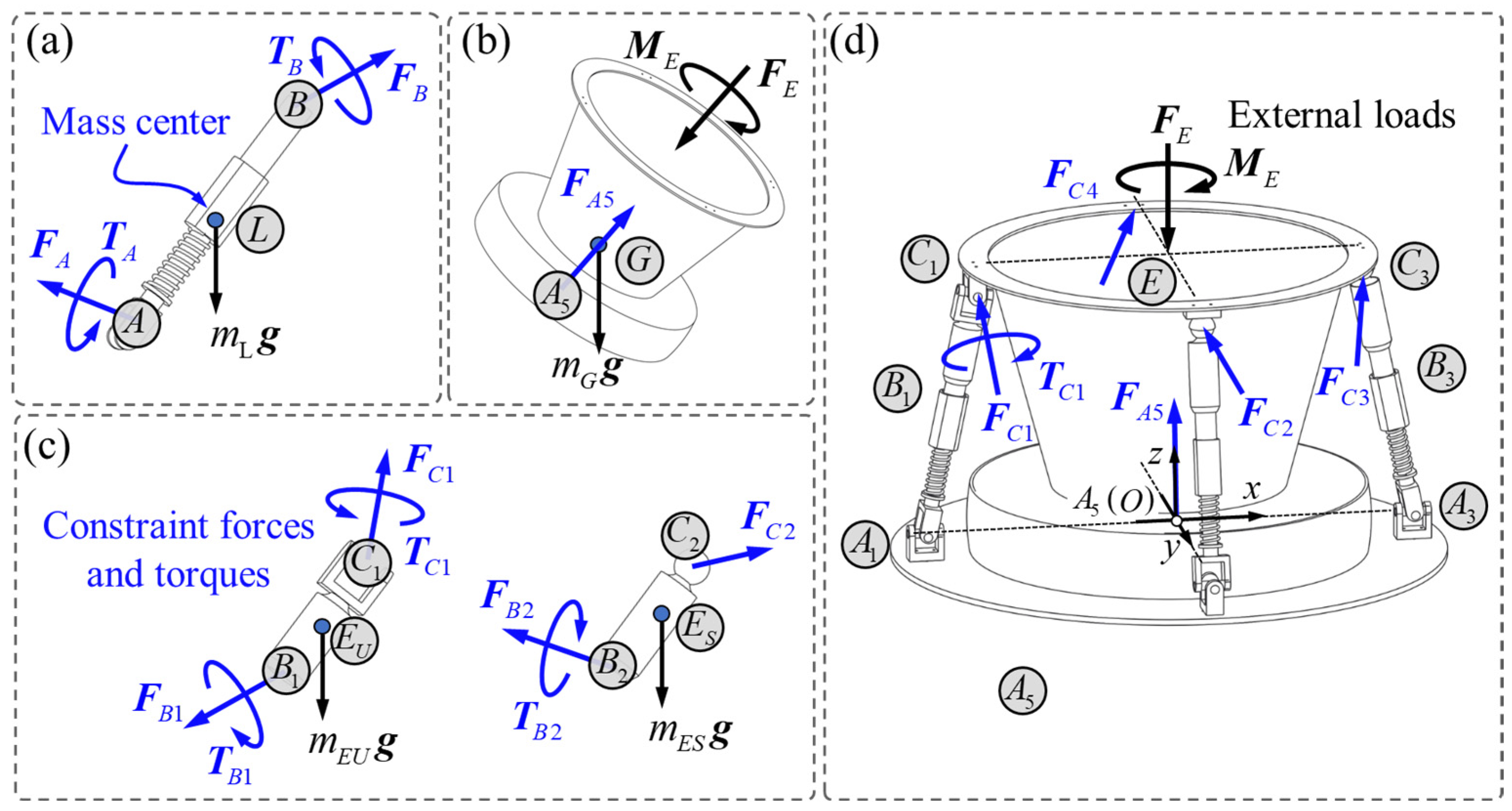
As shown in Figure 6a, the lower limbs of four subchains contain one universal joint and one prismatic joint, the momentum screw of the lower limbs can be derived as:

$${\cancel{\mathit{S}}}_M^L=\left[\begin{array}{c}\mathit{p}\\ {\mathit{r}}_C\times \mathit{p}+{\mathit{J}}_C\mathit{\omega }\end{array}\right]=\left[\begin{array}{c}{m}_L\left({\mathit{\omega }}_i\times {\mathit{r}}_i^L\right)\\ {}_O{\mathit{J}}_i^L{\mathit{\omega }}_i\end{array}\right] (i=1,2,3,4)$$

(40)

where ${}_O{\mathit{J}}_{}^L={\mathit{R}}_O{\mathit{J}}_{}^L{\mathit{R}}_O^{\mathrm{T}}+m_L\left[\left({\mathit{r}}_L^{\mathrm{T}}{\mathit{r}}_L\right)\mathit{I}-\left({\mathit{r}}_L{\mathit{r}}_L^{\mathrm{T}}\right)\right]$ is the inertia matrix of lower limbs in the absolute coordinate system with the transformation matrix from the local coordinate frame to the absolute coordinate frame ${\mathit{R}}_O$ and the inertia matrix of lower limbs ${\mathit{J}}_{}^L$ in their respective local coordinate frame. $\mathit{r}$ presents the position vector of the mass center of each limb in the absolute coordinate frame.

The force screw of the lower limbs in general form can be written based on Equation (30) as

$${}_O{\cancel{\mathit{S}}}_F^L=\left[\begin{array}{c}{\mathit{F}}_{Ai}+{\mathit{F}}_{Bi}+m_L\mathit{g}\\ {\mathit{r}}_{Ai}\times {\mathit{F}}_{Ai}+{\mathit{T}}_{Ai}+{\mathit{r}}_{Bi}\times {\mathit{F}}_{Bi}+{\mathit{T}}_{Bi}+{\mathit{r}}_{Li}\times m_L\mathit{g}\end{array}\right] (i=1,2,3,4)$$

(41)

Then, according to Equation (37) the momentum screw equation of four lower limbs can be obtained

$$\frac{\mathrm{d}}{\mathrm{d}t}\left[\begin{array}{c}{m}_L\left({\mathit{\omega }}_i\times {\mathit{r}}_i^L\right)\\ {}_O{\mathit{J}}_i^L{\mathit{\omega }}_i\end{array}\right]=\left[\begin{array}{c}{\mathit{F}}_{Ai}+{\mathit{F}}_{Bi}+m_L\mathit{g}\\ {\mathit{r}}_{Ai}\times {\mathit{F}}_{Ai}+{\mathit{T}}_{Ai}+{\mathit{r}}_{Bi}\times {\mathit{F}}_{Bi}+{\mathit{T}}_{Bi}+{\mathit{r}}_{Li}\times m_L\mathit{g}\end{array}\right] (i=1,2,3,4)$$

(42)

Similarly, the upper limbs of four subchains contains prismatic joint and universal joint or spherical joints, which is shown in Figure 6c, the momentum screw can be written as

$$\begin{array}{l}{\cancel{\mathit{S}}}_M^{EU}=\left[\begin{array}{c}\mathit{p}\\ {\mathit{r}}_C\times \mathit{p}+{\mathit{J}}_C\mathit{\omega }\end{array}\right]=\left[\begin{array}{c}{m}_{EU}{\mathit{v}}_{EU}+m_{EU}\left({\mathit{\omega }}_1^{EU}\times {\mathit{r}}_1^{EU}\right)\\ {}_O{\mathit{J}}_1^{EU}{\mathit{\omega }}_1^{EU}\end{array}\right] \\ {\cancel{\mathit{S}}}_M^{ES}=\left[\begin{array}{c}\mathit{p}\\ {\mathit{r}}_C\times \mathit{p}+{\mathit{J}}_C\mathit{\omega }\end{array}\right]=\left[\begin{array}{c}{m}_{ES}{\mathit{v}}_{ES}+m_{ES}\left({\mathit{\omega }}_i^{ES}\times {\mathit{r}}_i^{ES}\right)\\ {}_O{\mathit{J}}_i^{ES}{\mathit{\omega }}_i^{ES}\end{array}\right] (i=2,3,4)\end{array}$$

(43)

The force screw of the upper limbs of four subchains are

$$\begin{array}{l}{}_O{\cancel{\mathit{S}}}_F^{EU}=\left[\begin{array}{c}{\mathit{F}}_{B1}+{\mathit{F}}_{C1}+m_{EU}\mathit{g}\\ {\mathit{r}}_{B1}\times {\mathit{F}}_{B1}+{\mathit{T}}_{B1}+{\mathit{r}}_{C1}\times {\mathit{F}}_{C1}+{\mathit{T}}_{C1}+{\mathit{r}}_1^{EU}\times m_{EU}\mathit{g}\end{array}\right]\\ {}_O{\cancel{\mathit{S}}}_F^{ES}=\left[\begin{array}{c}{\mathit{F}}_{Bi}+{\mathit{F}}_{Ci}+m_{ES}\mathit{g}\\ {\mathit{r}}_{Bi}\times {\mathit{F}}_{Bi}+{\mathit{T}}_{Bi}+{\mathit{r}}_{Ci}\times {\mathit{F}}_{Ci}+{\mathit{r}}_i^{ES}\times m_{ES}\mathit{g}\end{array}\right] (i=2,3,4)\end{array}$$

(44)

The momentum screw of the moving platform can be deduced as:

$${\cancel{\mathit{S}}}_M^G=\left[\begin{array}{c}\mathit{p}\\ {\mathit{r}}_C\times \mathit{p}+{\mathit{J}}_C\mathit{\omega }\end{array}\right]=\left[\begin{array}{c}{m}_G{\mathit{v}}_G\\ {\mathit{r}}_G\times \left(m_G{\mathit{v}}_G\right){+}_O{\mathit{J}}_G{\mathit{\omega }}_G\end{array}\right]$$

(45)

where ${\mathit{r}}_G$ is the position vector of mass center $G$ of the moving platform in the absolute coordinate frame.

The moving platform consists of one universal pair and four spherical pairs, which are shown in Figure 6d. The force screw of the moving platform is

$${\cancel{\mathit{S}}}_F^G=\left[\begin{array}{c}{\displaystyle \sum _{i=1}^4{\mathit{F}}_{Ci}+{\mathit{F}}_{A5}+m_G\mathit{g}+{\mathit{F}}_E}\\ {\displaystyle \sum _{i=1}^4\left({\mathit{r}}_{Ci}\times {\mathit{F}}_{Ci}\right)+{\mathit{T}}_{C1}+{\mathit{r}}_G\times m_G\mathit{g}+{\mathit{M}}_E}\end{array}\right]$$

(46)

Therefore, the momentum screw equation of the moving platform can be written as

$$\frac{\mathrm{d}}{\mathrm{d}t}\left[\begin{array}{c}{m}_G{\mathit{v}}_G\\ {\mathit{r}}_G\times \left(m_G{\mathit{v}}_G\right){+}_O{\mathit{J}}_G{\mathit{\omega }}_G\end{array}\right]=\left[\begin{array}{c}{\displaystyle \sum _{i=1}^4{\mathit{F}}_{Ci}+{\mathit{F}}_{A5}+m_G\mathit{g}+{\mathit{F}}_E}\\ {\displaystyle \sum _{i=1}^4\left({\mathit{r}}_{Ci}\times {\mathit{F}}_{Ci}\right)+{\mathit{T}}_{C1}+{\mathit{r}}_G\times m_G\mathit{g}+{\mathit{M}}_E}\end{array}\right]$$

(47)

By associating the momentum screw equations, the dynamic equation of $3\mathrm{UPS}-\mathrm{UPU}-\mathrm{S}$ parallel mechanism can be deduced based on Equation (47)

$$\left[\begin{array}{c}{\displaystyle \sum _{i=1}^4{\mathit{F}}_{Ci}+{\mathit{F}}_{A5}}\\ {\displaystyle \sum _{i=1}^4\left({\mathit{r}}_{Ci}\times {\mathit{F}}_{Ci}\right)+{\mathit{T}}_{C1}}\end{array}\right]=\frac{\mathrm{d}}{\mathrm{d}t}\left[\begin{array}{c}{m}_G{\mathit{v}}_G\\ {\mathit{r}}_G\times \left(m_G{\mathit{v}}_G\right){+}_O{\mathit{J}}_G{\mathit{\omega }}_G\end{array}\right]-\left[\begin{array}{c}{m}_G\mathit{g}+{\mathit{F}}_E\\ {\mathit{r}}_G\times m_G\mathit{g}+{\mathit{M}}_E\end{array}\right]$$

(48)

Afterwards, the driven forces at prismatic joints at points $B_i (i=1,2,3,4)$ can be obtained through Equations (43) and (44):

$$\begin{array}{l}{\mathit{F}}_{B1}=\frac{\mathrm{d}}{\mathrm{d}t}\left[m_U{\mathit{v}}_U+m_U\left({\mathit{\omega }}_1^U\times {\mathit{r}}_1^{EU}\right)\right]-{\mathit{F}}_{C1}-m_U\mathit{g}\\ {\mathit{F}}_{Bi}=\frac{\mathrm{d}}{\mathrm{d}t}\left[m_E{\mathit{v}}_E+m_E\left({\mathit{\omega }}_i^S\times {\mathit{r}}_i^{ES}\right)\right]-{\mathit{F}}_{Ci}+m_E\mathit{g} (i=2,3,4)\end{array}$$

(49)

5. Numerical Simulation and Results Analysis

5.1. The Inverse Kinematics of the 3UPS-UPU-S Parallel Mechanism

To validate the efficiency of the kinematic and dynamic analysis methods proposed in this paper, a spatial trajectory is given for the moving platform. The function of trajectory over time is defined as

$$\{\begin{array}{l}x(t)=0.1\cos (t)+0.2, \left(\mathrm{m}\right)\\ y(t)=0.1\sin (t), \left(\mathrm{m}\right)\\ z(t)=H, \left(\mathrm{m}\right)\end{array}$$

(50)

Through the trajectory, the displacement vector ${\mathit{D}}_E$, velocity screw ${\cancel{\mathit{S}}}_E$, and acceleration vector ${\mathit{A}}_E$ of the moving platform are that:

$$\{\begin{array}{l}{\mathit{D}}_E={\left[\begin{array}{cccccc}0.1\cos (t)+0.2& 0.1\sin (t)& 0& 0& 0& H\end{array}\right]}^{\mathrm{T}}\left(\mathrm{m}\right)\\ {\mathit{V}}_E={\left[\begin{array}{cccccc}-0.1\sin (t)& 0.1\cos (t)& 0& 0& 0& 0\end{array}\right]}^{\mathrm{T}}\left(\mathrm{m}/\mathrm{s}\right)\\ {\mathit{A}}_E={\left[\begin{array}{cccccc}0.1\cos (t)& 0.1\sin (t)& 0& 0& 0& 0\end{array}\right]}^{\mathrm{T}}\left({\mathrm{m}/\mathrm{s}}^2\right)\end{array}$$

(51)

$t$ in Equations (50) and (51) is the time of the trajectory, the simulation step length is $\Delta t=0.001$ and the total number of iterations is $n=10000$. As depicted in Figure 1, $H$ is the initial height between the geometric center $O$ on the base platform and the geometric center E of the outer ring of the moving platform, $L$ is the initial length between joint $A$ and joint $C$. $R$ and $r$ are the constant radii of circle $A_1{A}_2{A}_3{A}_4$ and $C_1{C}_2{C}_3{C}_4$ formed by the primary universal joints and end universal/spherical joints of four kinematic subchains. $\theta$ and $p$ give the initial assembly configurations of each kinematic joint in four kinematic chains. The configuration parameters and the initial assembly configuration parameters of the $3\mathrm{U}\underset{\_}{\mathrm{P}}\mathrm{S}-\mathrm{U}\underset{\_}{\mathrm{P}}\mathrm{U}-\mathrm{S}$ parallel mechanism for kinematics analysis are given in

Table 1. Configuration parameters of the $3\mathrm{U}\underset{\_}{\mathrm{P}}\mathrm{S}-\mathrm{U}\underset{\_}{\mathrm{P}}\mathrm{U}-\mathrm{S}$.

$H\left(0\right) \left(\mathrm{m}\right)$	$R \left(\mathrm{m}\right)$	$r \left(\mathrm{m}\right)$	$L\left(0\right) \left(\mathrm{m}\right)$
$\frac{3\sqrt{3}}{10}$	$0.8$	$0.5$	$0.6$

and

Table 2. Initial conditions of the $3\mathrm{U}\underset{\_}{\mathrm{P}}\mathrm{S}-\mathrm{U}\underset{\_}{\mathrm{P}}\mathrm{U}-\mathrm{S}$.

${\theta }_1^i\left(0\right) \left(\mathrm{rad}\right)$	${\theta }_2^i\left(0\right) \left(\mathrm{rad}\right)$	$p_3^i\left(0\right) \left(\mathrm{m}\right)$	${\theta }_4^i\left(0\right) \left(\mathrm{rad}\right)$	${\theta }_5^i\left(0\right) \left(\mathrm{rad}\right)$	${\theta }_6^i\left(0\right) \left(\mathrm{rad}\right)$
$\left\{{\theta }_1^1\right\}=\left\{0\right\}$	$\left\{{\theta }_2^1\right\}=\left\{-\frac{\pi }{6}\right\}$	$\left\{p_3^1\right\}=\left\{0.3\right\}$	$\left\{{\theta }_4^1\right\}=\left\{0\right\}$	$\left\{{\theta }_5^1\right\}=\left\{-\frac{\pi }{3}\right\}$	$\left\{{\theta }_6^1\right\}=\left\{0\right\}$

, respectively.

The inverse kinematics of the $3\mathrm{U}\underset{\_}{\mathrm{P}}\mathrm{S}-\mathrm{U}\underset{\_}{\mathrm{P}}\mathrm{U}-\mathrm{S}$ parallel mechanism are programmed and carried out based on the given trajectory, and the curves of the kinematics are plotted and shown in Figure 7 and Figure 8.

Figure 7a plots the relative angular displacements $\theta$ of each revolute joint in five kinematic subchains. Figure 7b shows the relative linear displacements $d$ of all prismatic pairs of four subchains surrounding the moving platform.

Figure 8a depicts the relative angular velocity $\omega$ of each revolute joint in $3\mathrm{U}\underset{\_}{\mathrm{P}}\mathrm{S}-\mathrm{U}\underset{\_}{\mathrm{P}}\mathrm{U}-\mathrm{S}$ parallel mechanism. Figure 8b shows the relative linear velocity $v_3$ of four active prismatic pairs in four {UPU} and {UPS} subchains. According to the simulation results, there are no unexpected sudden changes in velocities, and the motion of each joint shows a harmonious operation of the mechanism.

5.2. The Inverse Dynamics of the $3U\underset{\_}{P}S-U\underset{\_}{P}U-S$ Parallel Mechanism

Suppose that the resultant action of the external mechanical loadings is acting on the geometric center of the outer ring of the moving platform at point $E$. The given resultant force is ${\mathit{F}}_E=\left[\begin{array}{ccc}0& 0& 1\end{array}\right] \left(\mathrm{kN}\right)$ and the resultant moment is ${\mathit{T}}_E=\left[\begin{array}{ccc}1& 0& 0\end{array}\right] \left(\mathrm{kN}\cdot \mathrm{m}\right)$. By utilizing the kinematic parameters of each joint obtained in Section 5.1, the inverse dynamic analysis of the $3\mathrm{U}\underset{\_}{\mathrm{P}}\mathrm{S}-\mathrm{U}\underset{\_}{\mathrm{P}}\mathrm{U}-\mathrm{S}$ parallel mechanism could be carried out, and the driving forces, which should be provided by four prismatic joints, could be gained through the approach introduced in Section 4. The needed structure parameters are illustrated in

Table 3. The structure parameters at the mass center of each limb and moving platform.

$\mathrm{Mass} \left(\mathrm{kg}\right)$
$\mathrm{Lower} \mathrm{limb} m_L$	$\mathrm{Upper} \mathrm{limb} m_{EU}$$, m_{ES}$	$\mathrm{Moving} \mathrm{platform} m_G$
1.42	1.42	2.87
$\mathrm{Moment} \mathrm{of} \mathrm{inertia} \mathrm{matrix} \left(\mathrm{kg}\cdot {\mathrm{m}}^2\right)$
$\mathrm{Lower} \mathrm{limb} {\mathbf{J}}_L$	$\mathrm{Upper} \mathrm{limb} {\mathbf{J}}_{EU}$$, {\mathbf{J}}_{ES}$	$\mathrm{Lower} \mathrm{limb} {\mathbf{J}}_G$
$\mathrm{diag}\left(\begin{array}{ccc}0.0556& 1.14& 1.16\end{array}\right)$	$\mathrm{diag}\left(\begin{array}{ccc}0.0556& 1.14& 1.16\end{array}\right)$	$\mathrm{diag}\left(\begin{array}{ccc}68.7& 68.7& 92.1\end{array}\right)$

.

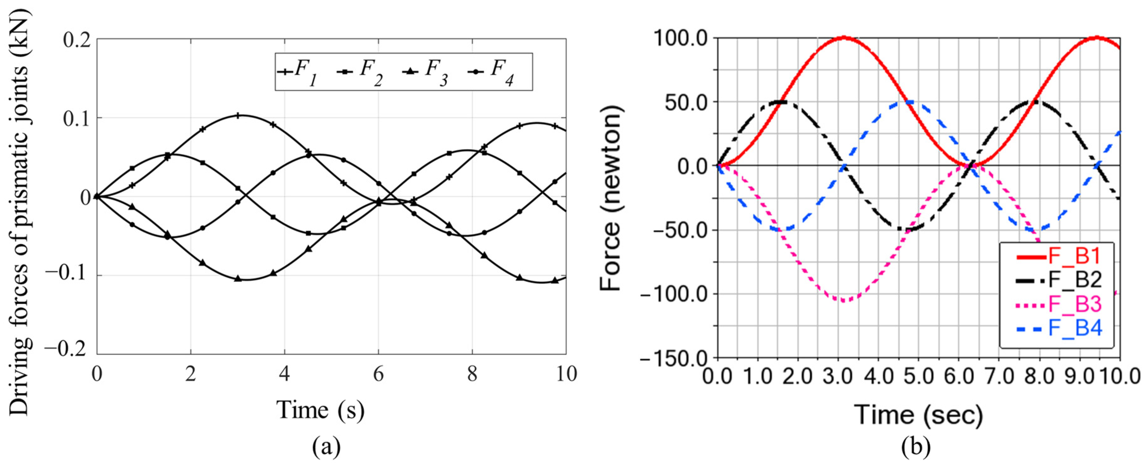
The whole kinematic and dynamic calculation process can be programmed. The driving forces exerted by the four prismatic joints are depicted in Figure 9, providing valuable insights into the dynamics of the system. Throughout the entire motion cycle, the resultant driving forces exhibit variations, and the forces generated by the four actuators are comparable in magnitude. This observation signifies that the actuators in the four prismatic joints are involved in achieving the determined motion through the whole motion cycle. Moreover, the forces required to keep balance from the external loads by the four actuators exhibit uniformity in terms of magnitude. This uniformity in force generation among the actuators reflects effective coordination, ensuring synchronized operation. Consequently, this effective coordination among the actuators contributes to an optimized distribution of external loads. The system’s ability to achieve a balanced load distribution is of paramount importance, as it guarantees the equitable sharing of external forces and facilitates the smooth functioning of the mechanism. The results indicate the effectiveness of the two additional {UPS} subchains. The simulation results of displacements and the forces of actuators during the given motion cycle can provide initial guidance for the selection and configuration of actuators.

To validate the correctness of the modeling method proposed here, dynamic analysis modeling based on Newton–Euler equations is also established [5]. Method A represents the method using momentum screws and force screws proposed in this paper, and Method B is the method based on Newton–Euler equations. From Figure 9, the results of both methods are consistent, which indicates the correctness of both methods. Furthermore, a dynamic analysis is performed by commercial software, Adams. The kinematic parameters of the specified motion are defined in Adams simulation model, and the driving forces of four actuators in prismatic joints are analyzed. The results of numerical analysis through MATLAB shown in Figure 10a and the results of simulation through Adams shown in Figure 10b are comparable and have good consistency. The simulation model used in Adams is simplified, and the influence of step length on simulation results has different weights in MATLAB and Adams, which can result in differences between the results.

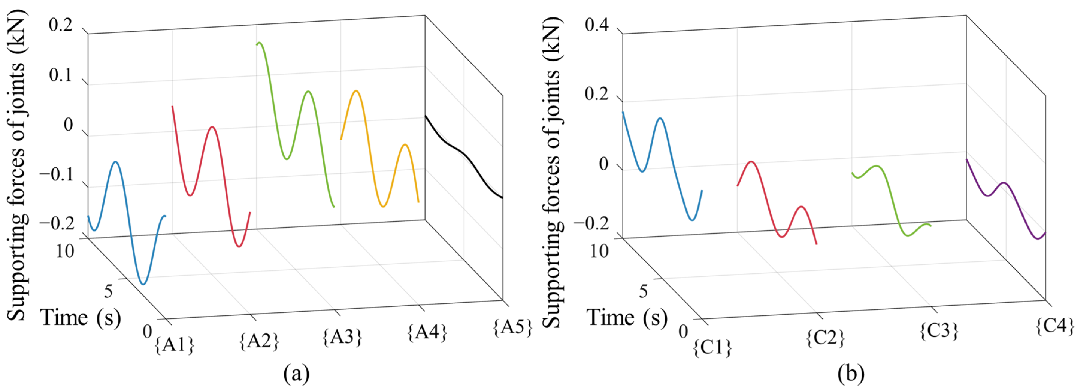
Besides all the driving forces, the support forces on each passive joint can be computed simultaneously. The forces exerted on universal joints assembled on the base at position $A_1, A_2, A_3, A_4$ and the spherical joint at position $A_5$ of the 5th kinematic chain are illustrated in Figure 11a. It shows that the four surrounding subchains withstand more forces than the chain {S}, which facilitates rotation of the spherical joint of chain {S} and allows for more stable motion overall. Figure 11b demonstrates the forces acting on universal joints at position $C_1$ and spherical joints $C_2, C_3, C_4$. In the whole motion period, forces vary according to the motion, and there are no sudden changes in forces, which expresses a stable and robust support.

The supporting forces on each joint can be measured by force sensors and employed in controlling the mechanism. The sensors should be arranged according to the working situation and other limitations, such as temperature and space limitations. By solving all the forces and torques of each joint, it provides the possibilities for designing various sensor arrangement schemes.

6. Conclusions

In this paper, a redundant actuated parallel mechanism with five kinematic subchains is introduced. The kinematics and dynamics of this mechanism are investigated in screw coordinates using the principle of screw theory. Firstly, the kinematic parameters of each kinematic joint within the mechanism, crucial for dynamic analysis, can be directly derived through velocity screws. Then, a dynamic modeling approach using momentum screws is proposed. Compared with conventional analysis methods like establishing Newton-Euler equations, employing momentum in screw form offers significantly improved computational efficiency and provides a clearer physical explanation of the equilibrium and control of multi-body systems. By utilizing screw coordinates, the coordination of kinematics and dynamics is achieved on a unified platform. Leveraging the kinematic information, the dynamic analysis can be carried out through the differential equations from the momentum screws and force screws, enabling simultaneous determination of the relevant forces and torques. Simulation results depict that the kinematics of each joint within this parallel mechanism can be initially solved based on the given motion of the manipulator. Additionally, the moving distance and required driving forces of each prismatic joint throughout the motion cycle can also be derived, offering essential information for actuator selection and configuration. Furthermore, the simulation results facilitate further optimization of the mechanism, such as controlling driving forces and torques within acceptable ranges. This method provides possibilities for the development of computational algorithms for dynamic analysis applicable to different types of mechanisms, including planar and spatial, as well as serial and parallel mechanisms.

References

- Zhao, J.-S.; Wei, S.-T.; Sun, H.-L. Kinematics and Statics of a 3-UPU Robot in Screw Coordinates. J. Mech. Robot. 2023, 15, 061004. [Google Scholar] [CrossRef]
- Chen, X.; Wu, L.; Deng, Y.; Wang, Q. Dynamic Response Analysis and Chaos Identification of 4-UPS-UPU Flexible Spatial Parallel Mechanism. Nonlinear Dyn. 2017, 87, 2311–2324. [Google Scholar] [CrossRef]
- Liu, S.; Peng, G.; Gao, H. Dynamic Modeling and Terminal Sliding Mode Control of a 3-DOF Redundantly Actuated Parallel Platform. Mechatronics 2019, 60, 26–33. [Google Scholar] [CrossRef]
- Chen, M.; Zhang, Q.; Qin, X.; Sun, Y. Kinematic, Dynamic, and Performance Analysis of a New 3-DOF over-Constrained Parallel Mechanism without Parasitic Motion. Mech. Mach. Theory 2021, 162, 104365. [Google Scholar] [CrossRef]
- Zhao, J.-S.; Wei, S.-T.; Sun, X.-C. Dynamics of a 3-UPS-UPU-S Parallel Mechanism. Appl. Sci. 2023, 13, 3912. [Google Scholar] [CrossRef]
- Chen, X.; Li, Y. Dynamics Analysis of Spatial Parallel Mechanism with Irregular Spherical Joint Clearance. Shock Vib. 2019, 2019, 6242971. [Google Scholar] [CrossRef]
- Asadi, F.; Heydari, A. Analytical Dynamic Modeling of Delta Robot with Experimental Verification. Proc. Inst. Mech. Eng. Part K J. Multi-Body Dyn. 2020, 234, 623–630. [Google Scholar] [CrossRef]
- Zhang, C.; Jiang, H. Rigid-Flexible Modal Analysis of the Hydraulic 6-DOF Parallel Mechanism. Energies 2021, 14, 1604. [Google Scholar] [CrossRef]
- Niu, A.; Wang, S.; Sun, Y.; Qiu, J.; Qiu, W.; Chen, H. Dynamic Modeling and Analysis of a Novel Offshore Gangway with 3UPU/UP-RRP Series-Parallel Hybrid Structure. Ocean Eng. 2022, 266, 113122. [Google Scholar] [CrossRef]
- Mazare, M.; Taghizadeh, M.; Najafi, M.R. Inverse Dynamic of a 3-P[2(US)] Translational Parallel Robot. Robotica 2019, 37, 708–728. [Google Scholar] [CrossRef]
- Yun, Y.; Li, Y. A General Dynamics and Control Model of a Class of Multi-DOF Manipulators for Active Vibration Control. Mech. Mach. Theory 2011, 46, 1549–1574. [Google Scholar] [CrossRef]
- Wen, S.; Qin, G.; Zhang, B.; Lam, H.K.; Zhao, Y.; Wang, H. The Study of Model Predictive Control Algorithm Based on the Force/Position Control Scheme of the 5-DOF Redundant Actuation Parallel Robot. Robot. Auton. Syst. 2016, 79, 12–25. [Google Scholar] [CrossRef]
- Mirtaheri, S.M.; Zohoor, H. Efficient Formulation of the Gibbs–Appell Equations for Constrained Multibody Systems. Multibody Syst. Dyn. 2021, 53, 303–325. [Google Scholar] [CrossRef]
- Mirtaheri, S.M.; Zohoor, H. The Explicit Gibbs-Appell Equations of Motion for Rigid-Body Constrained Mechanical System. In Proceedings of the 2018 6th RSI International Conference on Robotics and Mechatronics (IcRoM), Tehran, Iran, 23–25 October 2018; pp. 304–309. [Google Scholar]
- Pappalardo, C.M. Dynamic Analysis of Planar Rigid Multibody Systems Modeled Using Natural Absolute Coordinates. Appl. Comput. Mech. 2018, 12, 73–110. [Google Scholar] [CrossRef]
- Gallardo, J.; Rico, J.M.; Frisoli, A.; Checcacci, D.; Bergamasco, M. Dynamics of Parallel Manipulators by Means of Screw Theory. Mech. Mach. Theory 2003, 38, 1113–1131. [Google Scholar] [CrossRef]
- Gallardo-Alvarado, J.; Rodríguez-Castro, R.; Delossantos-Lara, P.J. Kinematics and Dynamics of a 4-P RUR Schönflies Parallel Manipulator by Means of Screw Theory and the Principle of Virtual Work. Mech. Mach. Theory 2018, 122, 347–360. [Google Scholar] [CrossRef]
- Liu, Z.; Tao, R.; Fan, J.; Wang, Z.; Jing, F.; Tan, M. Kinematics, Dynamics, and Load Distribution Analysis of a 4-PPPS Redundantly Actuated Parallel Manipulator. Mech. Mach. Theory 2022, 167, 104494. [Google Scholar] [CrossRef]
- Pennock, G.R.; Oncu, B.A. Application of Screw Theory to Rigid Body Dynamics. J. Dyn. Syst. Meas. Control 1992, 114, 262–269. [Google Scholar] [CrossRef]
- Gallardo-Alvarado, J.; Aguilar-Nájera, C.R.; Casique-Rosas, L.; Pérez-González, L.; Rico-Martínez, J.M. Solving the Kinematics and Dynamics of a Modular Spatial Hyper-Redundant Manipulator by Means of Screw Theory. Multibody Syst. Dyn. 2008, 20, 307–325. [Google Scholar] [CrossRef]
- Müller, A. Screw and Lie Group Theory in Multibody Kinematics: Motion Representation and Recursive Kinematics of Tree-Topology Systems. Multibody Syst. Dyn. 2018, 43, 37–70. [Google Scholar] [CrossRef]
- Müller, A. Screw Theory—A Forgotten Tool in Multibody Dynamics. Proc. Appl. Math. Mech. 2017, 17, 809–810. [Google Scholar] [CrossRef]
Figure 1.
Geometry of the parallel mechanism: (a) structure in front view; (b) structure in top view.
Figure 2.
Swing angles and schematic diagram of motion.
Figure 3.
Kinematics of kinematic subchains in the parallel mechanism.
Figure 4.
Topological diagram and screws showing the constraints of the parallel mechanism.
Figure 5.
Theory of the momentum screw of a rigid body.
Figure 6.
Dynamic analysis of the parallel mechanism. (a) Dynamics of the lower limbs of four subchains; (b) dynamics of the {S} chain; (c) dynamics of upper limbs of four subchains connecting with universal joint or spherical joints; (d) dynamics of the moving platform.
Figure 7.
Displacement of each kinematic joint. (a) Relative angular displacements of each revolute joint; (b) relative linear displacement of each prismatic joints within each kinematic chain.
Figure 8.
Relative velocity of each joint. (a) Relative angular velocity of each revolute joint; (b) relative linear velocities of four prismatic joints within each kinematic chain.
Figure 9.
The required driving forces of the prismatic joints in four kinematic subchains in the parallel mechanism.
Figure 10.
The driving forces of the prismatic joints computed by Adams. (a) Driving forces of the prismatic joints computed by MATLAB; (b) driving forces of the prismatic joints simulated by Adams.
Figure 11.
Supporting forces on each joint. (a) Forces on universal joints at position A1, A2, A3, A4 and spher-ical joint at position A5; (b) forces on universal joint at position C1 and spherical joints C2, C3, C4.