

Discontinuous Control Algorithm for Buck Converter under Time-Varying Load and Input Voltage


V.A. Trapeznikov Institute of Control Sciences of RAS, 117997 Moscow, Russia
*
Author to whom correspondence should be addressed.
Machines 2023, 11(9), 890; https://doi.org/10.3390/machines11090890
Submission received: 26 July 2023
/
Revised: 24 August 2023
/
Accepted: 2 September 2023
/
Published: 5 September 2023
(This article belongs to the Special Issue Design, Analytical Modeling, Optimization, and Application of Motor Drives)
Abstract
:In this paper, the problem of the output voltage regulation of buck converters is considered. The novelty of the problem statement is that the external electric load and the input voltage of the converter are unknown bounded functions of a certain class. In particular, the external load equivalent scheme is similar to the successive connection of the inductive and resistive elements. In this case, the behavior of the load current is described by the differential equation with time-varying coefficients. In this equation, the equivalent inductance and resistance are described by unknown arbitrary bounded functions with several bounded derivatives. Under known bounds for these functions and their derivatives, the initial system can be transformed into the special form with smooth bounded perturbation. This disturbance is an unknown function, and its action channel differs from the input channel. Therefore, the influence on the unknown external load can not be compensated for directly by the control input. Due to this reason, the new control strategy is developed in the paper with the help of a “vortex” algorithm, which provides asymptotic convergence of the regulation error to zero in time. How to choose the converter parameters and the bounds for the input voltage to operate the closed-loop system properly are shown. The convergence proof is organized with the help of the Lyapunov function approach, and the transient rate is also estimated. The simulation results show the efficiency of the designed control law for the wide class of input voltage and electrical parameter functions. The proposed control scheme may be further used in electric drive systems.
1. Introduction
At present, power converters are widely used in industry, aerospace and everyday life [1,2,3,4,5]. The heart of each power converter is the electronic switching device, which has two stable states of operation. In the ON state, it provides current flowing through itself, and in the OFF state, it disconnects different parts of an electronic scheme. In this paper, the direct current to direct current converter (DC/DC) is investigated, and the transformation of the input voltage from the upper level to the lower one is considered. This type of converter is called a buck converter in the literature [3,5,6,7].
There is a wide range of methods applied to the buck converter control. The classical linear regulation technique is used in [8] under the condition of the output voltage perturbation, and an auto-tuning approach for proportional-integral-derivative gain parameters of the feedback is proposed. The unknown load resistance step variations and its compensation technique with the extension of the classical proportional-integral-derivative regulator is developed in [9]. The feedback tuning coefficients of the linear quadratic Gaussian regulator is implemented in [10] for the case of the variable switching frequency. The discontinuous control solutions are designed in [11,12,13,14]. The stability analysis of the buck converter operation via Filippov’s method is contributed in [11]. The sliding mode control technique is developed in [12,13]. A generalization of this method is described in [14], and the advantages of using the sliding controllers as compared with the conventional linear controllers are discussed through some case-study examples. The specific time optimal control is developed in [15], which provides stabilization for the acceptable step reference voltage changes. The predictive-based current controller (inner loop for the DC input current) and a proportional integral voltage controller (outer loop for the DC output voltage) is proposed in [16] for the PFC single-phase rectifier based on the versatile buck-boost converter. The discontinuous control algorithm with hysteresis and finite switching frequency is considered in [17], and the technique of the hysteresis size choice is described. The nonlinear PID controller is developed in [18] under the assumption that the input voltage is a piece-wise constant function of the time.
Generally speaking, the above-described publications [10,11,12,13,14,15,16,17,18] deal with the constant resistive load consideration only for the sake of simplicity. A non-resistive load actually requires the converter model to be modified and extended due to the presence of capacitive or inductive elements, which can accumulate electric or electromagnetic energy. One of the possible control laws is designed in [19] for the case of time-varying resistive and inductive loads. However, the problem of the output voltage stabilization of the DC/DC converter under unknown time-varying inductive and resistive load is the challenge control task.
This paper is devoted to the problem of buck converter control with time-varying inductive and resistive loads. There are several unsolved problems concerned with this challenge. The classical task of the buck converter control is to provide a constant output voltage level under resistive load. For the proposed load, there are several problems that are insufficiently studied in the literature, as discussed above.
- The inductive and resistive nature of the load yields the growth of the dynamical order of the control plant.
- The linear system with time-varying coefficients must be analyzed during feedback synthesis.
- The designed control algorithm must be suitable under insufficient information about load parameters and variable input voltage. In particular, the problem statement from [18] for the case of piece-wise constant input voltage may be extended for the situation of the arbitrary input voltage function.
This paper is devoted to the solution of the set of the challenges described above. It will be shown that the control plant may be transformed into the canonical form with unmatched perturbation [20,21]. To solve the problem of a disturbance compensation, the variable structure controller based on a “vortex”algorithm [22,23] is developed below. The Lyapunov function method [24,25,26] is used for transient behavior analysis.
The paper is organized as follows. In Section 2, the problem statement is considered, and the basic description of the control plant is described. In Section 3, the basic control algorithm is developed. In Section 3.1, the property of the energy dissipation is discussed for the system with zero control input, and one of the main lemmas is proven. The close loop system stability analysis is provided by means of the Lyapunov function method, and the main theorem is formulated in Section 3.2. The simulation results are presented in Section 4. Finally, in Section 5, some concluding remarks about the developed results are given.
2. Problem Statement
The qualitative scheme of the researched system is depicted in Figure 1.
The differential equations of the investigated system are [27,28]:
where the variables and parameters are defined in Table 1.
The following features of the control object are highlighted.
1. The functions describing the behavior of the load resistance and inductance fulfill the restrictions
where is the absolute value of a number, are known constants and by means of , , the i-th derivatives of the functions and are denoted, respectively.
2. The bounds for the input voltage and its derivative are assumed to be known
where are known positive constants.
3. The “latch”diode VD provides a non-negative current flowing only (see Figure 1). Further, in any real power converter, there are heat losses concerned with the active resistance r and the resistance of the switch. Due to this reason, the maximum converter current must be limited by some value. Therefore, there are two inequalities for the current , and the second one must be provided by the control input choice
where is the initial time, and is the maximum possible current level.
4. Variables are measured.
The regulation problem for load voltage is stated in the paper
where is the desired value of the load voltage.
3. Results
According to the electrical scheme of the investigated system, the inductor may be considered the current source for the external load. The parameters of the step-down converter may be chosen to provide a fast, transient response according to the variations in the consumer current. From the other point of view, the unknown load parameter’s changes must be compensated for by the appropriate control law choice. It is necessary to note that the influence of on the system behavior can not be attenuated directly by the control input because these signals are introduced in the different equations of system (1). Therefore, the stated problem, (6), is complicated by the challenge of the unmatched perturbation suppression [20,21].
With the help of (6), the system equations may be written in the following representation
where .
The alternative representation of (7) is
where , .
In this paper, it is proposed to separate the whole transient process into two main stages.
1. The first stage corresponds to the convergence of the state space vector of the system to some vicinity of the origin, where perturbation and its derivative are bounded. It will be shown below that this can be performed by choosing the control input . This part of the transient process is finished after the time interval , and the control input is
Lemma 1.
For the external load, the following condition is fulfilled
and the parameters of the converter are chosen according to inequalities
The proof of Lemma 1 is given in Section 3.1.
2. The second stage corresponds to the main part of the closed-loop system operation, at which the solution of the stated problem (6) is provided. It is seen that the transformed system (7) has the unmatched perturbation , which can not be directly suppressed by the control input with the help of the sliding mode technique or other methods. For this reason, the conception of the “vortex”algorithm [22] is used in this paper to provide asymptotic unmatched disturbance attenuation. From the other point of view, the converter current must be restricted according to (5). Combining the above, in the second part of the transient process, the control input is chosen in the form
where .
The convergence analysis of the second stage is considered below in this section.
3.1. Proof of Lemma 1
Proof of Lemma 1.
The following coordinate transformation is introduced for system (1)
The differential equations for the new variables are
Non-singlar case (). The derivative of the Lyapunov candidate function
according to (2) and (14)
where .
According to the Hurwitz criterion [29], matrix is a positive definite matrix if the determinant is positive
It follows from this condition that the following inequality must be fulfilled for the converter parameters
From (16), one can write the inequality
where is the minimal Eigenvalue of matrix , which is positive due to (10).
According to the basics of mathematical analysis [30,31], the local minimums of are reached at the extreme points calculated from the equation
After comparing the two numbers
with the help of the difference
one can conclude from (10) that and expression (18) is always negative. This means that is the decreasing function. Thus, reaches a minimum at the upper bound of according to (2)
Singular case (). In this situation, the right-hand side of the first equation of (1) is discontinuous, and the buck converter is loaded with resistance only. By means of the theory of a singular perturbed system [32], the first differential equation of the plant (1) is transformed into the algebraic equation for the set of the points
The minimal Eigenvalue of matrix is
Finally, from (20) and (25), one can obtain the Lyapunov function derivative estimation for the whole range of the inductance
where .
Lemma 1 is proved. □
3.2. Closed-Loop System Analysis
The “vortext”algorithm used in the feedback provides the convergence to zero if the perturbation and its derivative are bounded by some known constants [22]. It follows from (8) that and depend on the values of the load current and its first and second derivatives. The following lemma gives a useful result that justifies the boundedness of the mentioned variables.
Lemma 2.
There is time instant such that, for the arbitrary initial conditions of plant (1), the closed-loop system trajectories converge to the neighborhood
where
Proof of Lemma 2.
The equations for the first and the second derivatives of can be calculated from the first equation of (1)
The general solutions for the variables are derived from (1) and (31) by means of the method of variation in arbitrary variables [30,31,33]:
where the functions are calculated as the following
It is obvious that for the stability of solution (32), functions must be positive. According to this requirement, condition (10) of Lemma 1 is justified, taking into account (2).
From Lemma 1’s result, one can write the following estimations by using (2), (13), (15) and (27) for the time interval
where .
For the same time interval, the inequality for is achieved with the help of (32), (34) and (35)
where , , , denotes the derivative of function with respect to variable and is calculated according to the rule of differentiation of the integral by the upper limit [30,31,33]
The estimation for is written in a similar way by using (1), (32) and (34)–(36)
where , and values are calculated according to
The differential equation for variable can be written from (1)
According to (1), (32), (34)–(36) and (39), the exponential estimation for the second derivative inside time interval
where , and the values of are calculated according to
There are singularities in estimations (37) and (40) if . For this case, according to the theory of singular perturbed systems [32], the first equation of (1) and (31) degenerate into the system of the algebraic equations
It is seen from (36), (37) and (40) that variables tend to zero with . Therefore, the time instant can be chosen in such a way that belong to neighborhood (30). The convergence time to the specified vicinity of the origin for each variable can be estimated from (36), (37) and (40)
By using (44), the end time of the dissipation stage can be chosen according to the relation
For further analysis of the closed-loop system transient process, the following notations are introduced:
where corresponds to the overshoot of during the transient process. The coefficients are calculated as
The constants corresponding to the perturbation and its derivative are calculated as
where
The choice of bounds (46) and (47) will be justified during the main theorem proof formulated below.
Theorem 1.
Proof of Theorem.
According to Section 2, the normal operation regime of the buck converter corresponds to the positive values of the control plant (1) variables. Despite that, the negative initial values for variables and can not be excluded from stability analysis consideration. For the considered dynamic range (46) of variable , the transient regime must be investigated for the initial conditions that yield the maximum overshoot of the output error . From (35) and (36), the given margins for the absolute values of the plant variables are guaranteed. Therefore, we choose the negative initial value for the capacitor voltage and consider two possible scenarios of the transient process with appropriate initial conditions for the converter and load currents.
Further, the following notations are used:
- (1)
- is the time instant at which ;
- (2)
- is the time instant at which .
First, bound (46) is justified and overshoot is estimated.
Case 1.
During time interval , according to the conditions of Theorem 1,
the phase point rotates in the clockwise direction until it crosses axis .
The time instants are introduced in
With the help of (32)–(34), (51) and the inequality
the lower bound for variable inside time interval is
For the remaining time interval in the second quadrant of the phase plane, one can write with the help of (1), (28) and (50)
Let us introduce time instant such that
If variable for , then with the help of the first equation of (1), and (2), (53) and (54), the following inequalities are achieved
According to Lemma 1’s result, time instant can be chosen to provide the relation
which contradicts the assumption about the negativeness of from (56).
Case 2.
There is no time instant for this case. For time interval according to (32)–(34) and (61), the lower bound for variable inside the time interval is
Like in the previous case (59), the inequality
guarantees that the value and peak estimation (58) of from (46) is also valid for Case 2. Time instant is chosen by using (60).
From the practice point of view, to provide a necessary value of according to the conditions of Theorem 1, parameter r and the lower bound of must be chosen like this:
The estimation of the overshoot is based on the phase portrait analysis of system (28) depicted in Figure 2 or Figure 3. The maximum over-regulation of happens at time instant with the initial condition as was shown in (58). Due to the condition of Theorem 1
the phase point rotates in the clockwise direction with as it is depicted in Figure 2 and Figure 3.
For overshoot estimation the comparison system is introduced for
The tangents to the phase trajectories of systems (28) and (65) in the first quadrant of the phase plane (see Figure 2 and Figure 3) are written in the forms
By means of the expressions from Theorem 1
the arbitrary point located inside the first quadrant of the phase plane, the following inequality is derived
For the phase portraits starting from point
the curve 2 (see Figure 2 and Figure 3) is a majorant for the phase trajectory 1 of (28) for .
For the purpose of the maximum value of estimation, we write the first integral [30,33] from (65)
where is constant determined by the initial conditions (66).
Let us denote the time instant according to
At this point, equality (67), with the help of (47), can be rewritten in the form
By using the condition of Theorem 1 and (47), one can conclude that
The computed value of the overshoot corresponds to (46) introduced earlier.
The derived expression for is not explicit since it includes as a function of . Therefore, after the overshoot calculation, the condition of Theorem
must be checked.
By the substitution of (64) into (68) one can obtain the explicit solution of the overshoot as a function of the converter parameters and the desired output voltage with the help of the following equation
where
The positive solution of the last equation is
For further transient process analysis under , the new coordinates are used
and we rewrite system (28) to the form
where is calculated from (13).
The phase point of the closed-loop system (72) rotates in the clockwise direction, as depicted in Figure 4. The right-hand side of differential Equation (72) is discontinuous on the set of points . It is necessary to note that the phase curve goes through axis , and there is no sliding motion [12,13] along manifold . Due to this reason, the function (12) is determined in the Caratheodory sense [34]. Below, system (72)’s motion is investigated under .
The final part of Theorem 1 is proven by using the Lyapunov functions candidates
where .
First, case is considered. After performing the calculations according to (72) with , one can write
where .
Thus, according to the conditions of Theorem 1 , and , the system trajectories belong to the first and the fourth quadrants of the phase plane (see Figure 4).
By using (73), the following inequality is produced
where .
Simultaneously, under condition , the time derivative of according to the restrictions of (3) can be written as
where is positive according to the conditions of Theorem 1.
The following time intervals are introduced . After consideration of the phase portrait, using (75), (76), (78) and (79), the following estimates can be derived for number i
where , , , .
By using in the right half of the phase plane, the following inequalities can be derived
The upper bound estimation for the variable at time instant is
The extremes of happen under condition (see Figure 3) at time instants
The inequality for is
With the help of (80), one can conclude that
It follows from the proof of Theorem 1 that . Therefore, estimation (58) is valid for , and bounds (46) are justified for in the sense of (29) for . According to (30), the bounds for the derivative are calculated as in (46).
From (1), the differential inequality for the second derivative of the capacitor voltage is
due to positiveness of . Bounds (46) are checked fully.
Taking into account the expressions for the perturbation and its derivative
estimation (47) can be easily checked with the help of (46).
This concludes the proof of Theorem 1. □
4. Simulation Results
Experiment 1. For the numerical example, the parameters of the control plant and the output voltage are chosen according to Table 2.
The harmonic functions are used to describe the external load behavior and the input voltage variations:
The bounds for the time-varying functions in the form (2) are written as:
By using the data from Table 2, (81) and the initial conditions for plant (1) from Table 3, the following computations are made based on the referenced expressions:
- (1)
- (2)
- (3)
- (4)
- (5)
- (6)
The calculation results are listed in Table 3.
The following filters are introduced to show the low-frequency components of the corresponding signals
where is the filter parameter and are the smoothed signals of variables , respectively.
The simulation results of Experiment 1 with from Table 3 are depicted in Figure 5. The Dorman-Prince numerical integration method (ode 5) is used with sample time .
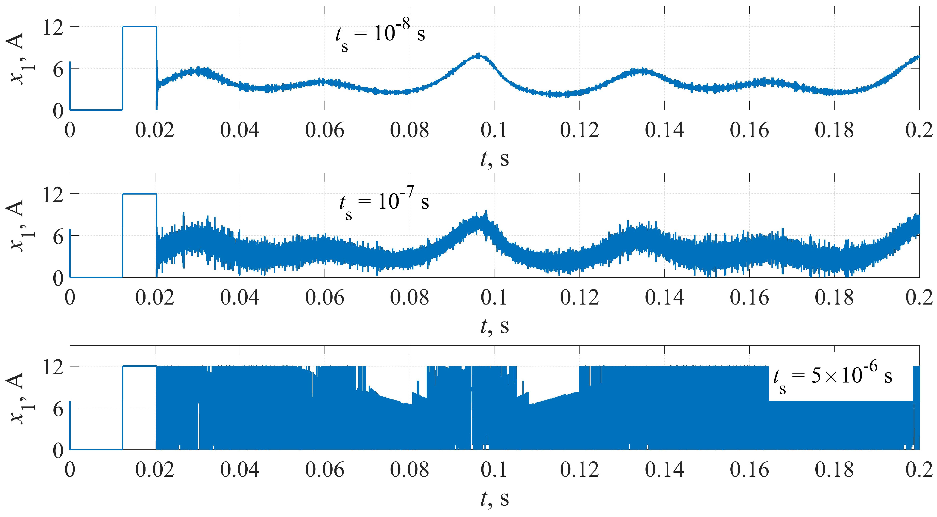
Experiment 2. For the second numerical example, several integration steps are used according to Table 4. The results of this experiment are depicted in Figure 6 and Figure 7. Due to finite switching frequency, there are high-frequency oscillations in the output voltage and the inductor current [35,36]. The maximum of the half of the difference between the local 392 peak and valley of the current oscillation is denoted as . Table 4 is filled by the maximum of the voltage regulation errors and data.
Theorem 1 declares that the output error converges to zero asymptotically. The switching period or ON/OFF time of the relay control inputs depends on the oscillation amplitude of variable . The lower oscillation amplitude yields a lower period or higher switching frequency. Therefore, for the infinite small oscillation amplitude, the switching frequency is infinitely large. In practice, the switching frequency is always upper bound [1,2,3,4,5]. It is seen that the smaller error corresponds to the smaller sample time or the smaller switching period. Therefore, in practice, the output voltage regulation accuracy depends on the switching frequency of the power switch. This is the main practical limitation of the designed control law. It is necessary to note that this restriction is similar to all existing control approaches.
5. Conclusions
In this paper, the problem of the output voltage stabilization of the down-step voltage converter has been studied. The class of functions that describes the behavior of the time-varying external load is introduced. It was shown that the closed-loop system stability can be provided by appropriate choices of the converter and controller parameters under sufficient lower bounds of the input voltage. The robustness and effectiveness of the designed control law is proven with the help of the Lyapunov method function. The solvability condition that guarantees the internal stability of the load current and its first two derivatives is derived for the considered class of load parameter functions. Future works may be devoted to finite switching frequency controller consideration, which will be used in practice. Another research branch may be concerned with electric drive control under time-varying load torque.
Author Contributions
Conceptualization, methodology, S.K. and V.A.U.; validation, investigation, formal analysis, S.K., S.A.K. and V.A.U.; writing—original draft preparation, S.K. and S.A.K.; writing—review and editing, S.A.K. and V.A.U. All authors have read and agreed to the published version of the manuscript.
Funding
This research received no external funding.
Institutional Review Board Statement
Not applicable.
Informed Consent Statement
Not applicable.
Data Availability Statement
Not applicable.
Conflicts of Interest
The authors declare no conflict of interest.
References
- Cho, Y.K.; Park, B.H.; Hyun, S.B. Delta-Sigma Modulator-Based Step-Up DC–DC Converter with Dynamic Output Voltage Scaling. Electronics 2020, 9, 498. [Google Scholar] [CrossRef]
- Dimitrov, B.; Hayatleh, K.; Barker, S.; Collier, G.; Sharkh, S.; Cruden, A. A Buck-Boost Transformerless DC–DC Converter Based on IGBT Modules for Fast Charge of Electric Vehicles. Electronics 2020, 9, 397. [Google Scholar] [CrossRef]
- Batarseh, I.; Harb, A. Power Electronics Circuit Analysis and Design, 2nd ed.; Springer: Berlin/Heidelberg, Germany, 2018. [Google Scholar]
- Bose, B.K. Modern Power Electronic and AC Drives; Prentice Hall PTR: Hoboken, NJ, USA, 2002. [Google Scholar]
- Wilamowski, B.M.; Irwin, J.D. Power Electronics and Motor Drives, 2nd ed.; CRC Press: New York, NY, USA, 2011. [Google Scholar]
- Tsai, C.T.; Chen, W. Buck Converter with Soft-Switching Cells for PV Panel Applications. Energies 2016, 9, 148. [Google Scholar] [CrossRef]
- Ostman, B.K.; Jrvenhaara, J.K. A Rapid Switch Bridge Selection Method for Fully Integrated DC/DC Buck Converters. IEEE Trans. Power Electron. 2015, 30, 4048–4051. [Google Scholar] [CrossRef]
- Stefanutti, W.; Mattavelli, P.; Saggini, S.; Ghioni, M. Autotuning of Digitally Controlled DC-DC Converters Based on Relay Feedback. IEEE Trans. Power Electron. 2007, 22, 199–207. [Google Scholar] [CrossRef]
- Sira-Ramirez, H.; Marquez, R.; Fliess, M. Generalized PI Sliding Mode Control of DC-to-DC Power Converters. IFAC Proc. Vol. 2001, 34, 699–704. [Google Scholar] [CrossRef]
- Priewasser, R.; Agostinelli, M.; Unterrieder, C.; Marsili, S.; Huemer, M. Modeling, Control, and Implementation of DC–DC Converters for Variable Frequency Operation. IEEE Trans. Power Electron. 2014, 29, 287–301. [Google Scholar] [CrossRef]
- Giaouris, D.; Banerjee, S.; Zahawi, B.; Pickert, P. Stability Analysis of the Continuous-Conduction-Mode Buck Converter Via Filippov’s Method. IEEE Trans. Circuit Syst. 2008, 55, 1084–1096. [Google Scholar] [CrossRef]
- Sabanovic, A.; Sabanovic, N.; Ohnishi, K. Sliding Mode in Power Converters and Motion Control Systems. Int. J. Control 1993, 57, 1237–1259. [Google Scholar] [CrossRef]
- Utkin, V.I. Sliding Mode Control in Electromechanical Systems; Tailor and Francis: London, UK, 2009. [Google Scholar]
- Tan, S.C.; Lai, Y.M.; Tse, C.K. General Design Issues of Sliding-Mode Controllers in DC–DC Converters. IEEE Trans. Power Electron. 2008, 55, 1160–1174. [Google Scholar]
- Kapat, S.; Krein, P.T. Improved time optimal control of a buck converter based on capacitor current. IEEE Trans. Power Electron. 2012, 27, 1444–1454. [Google Scholar] [CrossRef]
- González-Castaño, C.; Restrepo, C.; Sanz, F.; Chub, A.; Giral, R. DC Voltage Sensorless Predictive Control of a High-Efficiency PFC Single-Phase Rectifier Based on the Versatile Buck-Boost Converter. Sensors 2021, 21, 5107. [Google Scholar] [CrossRef]
- Hoyos Velasco, C.I.; Hoyos Velasco, F.E.; Candelo-Becerra, J.E. Nonlinear Dynamics and Performance Analysis of a Buck Converter with Hysteresis Control. Computation 2021, 9, 112. [Google Scholar] [CrossRef]
- Campos-Mercado, E.; Mendoza-Santos, E.F.; Torres-Muñoz, J.A.; Román-Hernández, E.; Moreno-Oliva, V.I.; Hernández-Escobedo, Q.; Perea-Moreno, A.J. Nonlinear Controller for the Set-Point Regulation of a Buck Converter System. Energies 2021, 14, 5760. [Google Scholar] [CrossRef]
- Ibarra, L.; Bastida, H.; Ponce, P.; Molina, A. Robust Control for Buck Voltage Converter Under Resistive and Inductive Varying Load. In Proceedings of the 13th International Conference on Power Electronics, Guanajuato, Mexico, 20–23 June 2016; pp. 126–131. [Google Scholar]
- Utkin, V.A. Invariance and Independence in Systems with Separable Motion. Autom. Remote Control 2001, 62, 1825–1843. [Google Scholar] [CrossRef]
- Wonham, W.M. Linear Multivariable Control: A Geometric Approach; Springer: New York, NY, USA, 1974. [Google Scholar]
- Kochetkov, S.A.; Utkin, V.A. Invariance in Systems with Unmatched Perturbations. Autom. Remote Control 2013, 74, 1097–1127. [Google Scholar] [CrossRef]
- Kochetkov, S.A.; Krasnova, S.A.; Utkin, V.A.; Vershinin, Y.A. Tracking Problem for Induction Electric Drive under Influence of Unknown Perturbation. IFAC-PapersOnLine 2017, 50, 9790–9795. [Google Scholar] [CrossRef]
- Zubov, V.I. Methods of A.M. Lyapunov and Their Application; Noordhoff Ltd.: Groningen, The Netherlands, 1964. [Google Scholar]
- Zubov, V.I. Analytic construction of Lyapunov functions. Dokl. Math. 1994, 49, 414–417. [Google Scholar]
- Dubljević, S.; Kazantzis, N. A new Lyapunov design approach for nonlinear systems based on Zubov’s method. Automatica 2002, 38, 1999–2007. [Google Scholar] [CrossRef]
- Johnson, D. Fundamentals of Electrical Engineering I; Connexions: Houston, TX, USA, 2016. [Google Scholar]
- Gross, C.A.; Roppel, T.A. Fundamentals of Electrical Engineering, 1st ed.; CRC Press: New York, NY, USA, 2012. [Google Scholar]
- Bellman, R. Introduction to Matrix Analysis, 2nd ed.; SIAM: Philadelphia, PA, USA, 1997. [Google Scholar]
- Piskunov, N. Differential and Integral Calculus; Mir Publishers: Moscow, Russia, 1969. [Google Scholar]
- Fikhtengol’ts, G.M. The Fundamentals of Mathematical Analysis: International Series of Monographs in Pure and Applied Mathematics, 72; Pergamon Press: Oxford, UK, 2016. [Google Scholar]
- Kevorkian, J.; Cole, J.D. Perturbation Methods in Applied Mathematics; Springer: New York, NY, USA, 1981. [Google Scholar]
- Teschl, G. Ordinary Differential Equations and Dynamical Systems; AMS: Providence, RI, USA, 2012. [Google Scholar]
- Filippov, A.F. Differential Equations with Discontinuous Right Hand Sides; Kluwer Academic Publishers: Dordrecht, The Netherlands, 1988. [Google Scholar]
- Bartolini, G.; Ferrara, A.; Usai, E. Chattering avoidance by second-order sliding mode control. IEEE Trans. Autom. Control 1998, 43, 241–246. [Google Scholar] [CrossRef]
- Fridman, L. An averaging approach to chattering. IEEE Trans. Autom. Control 2001, 46, 1260–1264. [Google Scholar] [CrossRef]
Figure 1.
The simplified scheme of the buck converter with the time-varying resistive and inductive load.
Figure 1.
The simplified scheme of the buck converter with the time-varying resistive and inductive load.

Figure 2.
The estimation of the maximum output voltage. 1—the phase portrait of the closed-loop system (28), 2—the phase portrait of the comparison system (65).
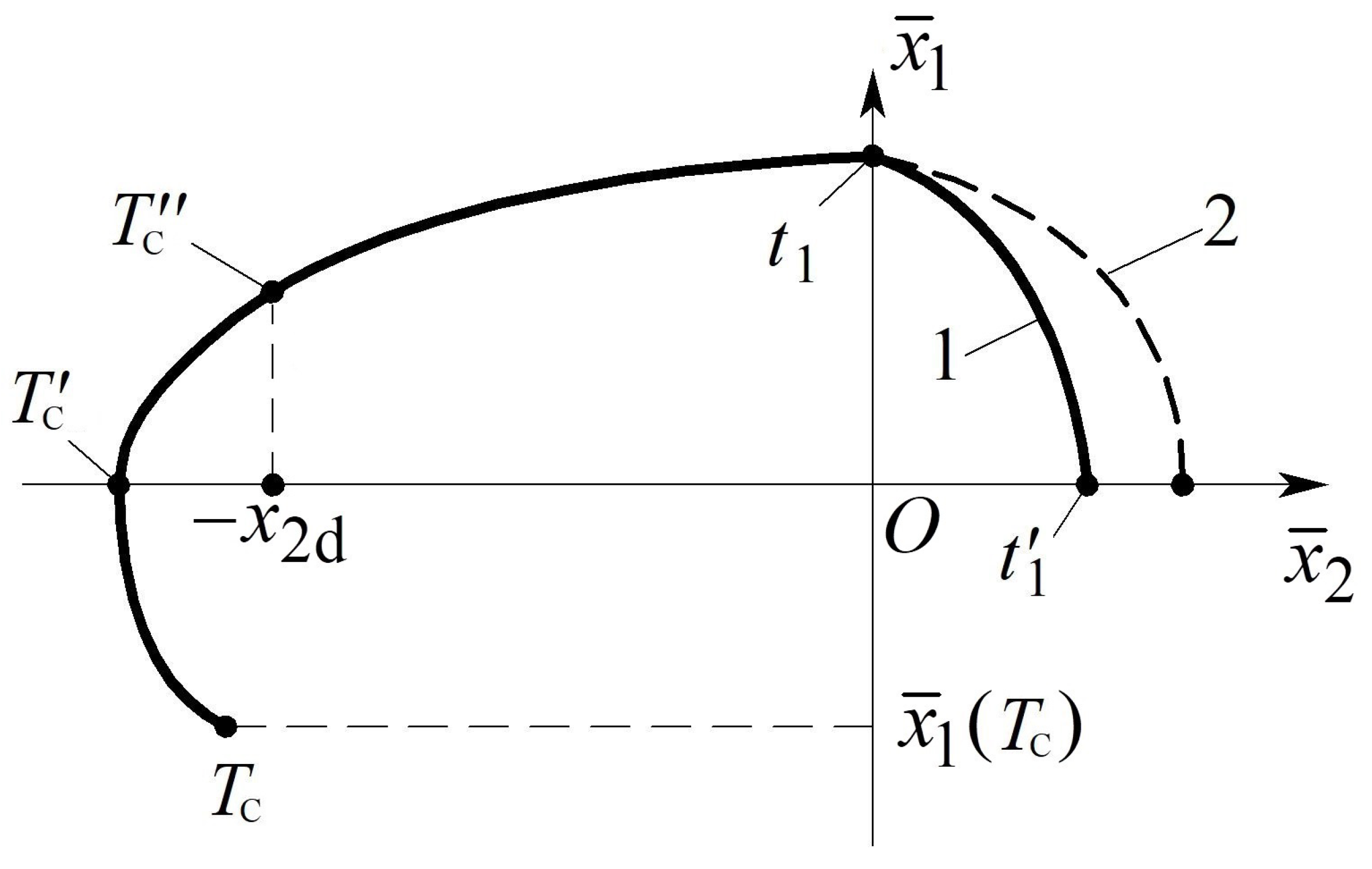
Figure 3.
The estimation of the maximum output voltage. 1—the phase portrait of the closed-loop system (28), 2—the phase portrait of the comparison system (65).
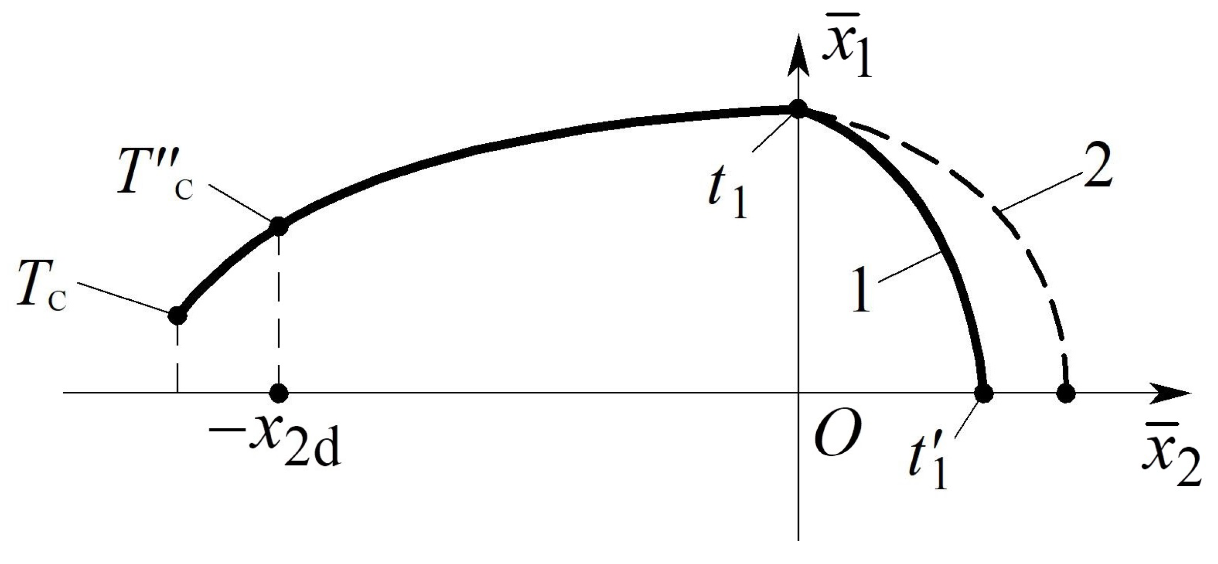
Figure 4.
Phase portrait of the closed-loop system.

Figure 5.
The simulation results of the closed-loop system (28). (a) Plots of ; (b) Plots of ; (c) Plot of ; (d) Plots of .
Figure 5.
The simulation results of the closed-loop system (28). (a) Plots of ; (b) Plots of ; (c) Plot of ; (d) Plots of .

Figure 6.
The steady—state output error at various integration steps.

Figure 7.
The inductor current graphs at various integration steps.

Table 1.
The variables and parameters definitions.
| Parameter/Variable | Definition |
|---|---|
| the inductor’s inductance | |
| the inductor’s active resistance | |
| the capacitor’s electrical capacity | |
| the variable load’s active resistance | |
| the variable load’s inductance | |
| the variable input’s voltage | |
| the inductor’s current | |
| the capacitor’s voltage | |
| the load’s current | |
| the electromotive force | |
| the control input |
Table 2.
The simulation parameters.
| 0.2 | 28 |
Table 3.
The parameters, coefficients and the variables’ bounds calculations.
| 7 | 15 | 912 | 456 | 345.45 | |||
| 218.2 | 204.13 | 21.43 | 2.4944 | 1.11 | |||
| 12 | 28.063 | 10.79 | 0 | ||||
| 0 | 909.1 |
Table 4.
The steady-state error and the current oscillations for several integration steps.
| 6 |
Disclaimer/Publisher’s Note: The statements, opinions and data contained in all publications are solely those of the individual author(s) and contributor(s) and not of MDPI and/or the editor(s). MDPI and/or the editor(s) disclaim responsibility for any injury to people or property resulting from any ideas, methods, instructions or products referred to in the content. |
© 2023 by the authors. Licensee MDPI, Basel, Switzerland. This article is an open access article distributed under the terms and conditions of the Creative Commons Attribution (CC BY) license (https://creativecommons.org/licenses/by/4.0/).
Share and Cite
MDPI and ACS Style
Krasnova, S.A.; Kochetkov, S.; Utkin, V.A. Discontinuous Control Algorithm for Buck Converter under Time-Varying Load and Input Voltage. Machines 2023, 11, 890. https://doi.org/10.3390/machines11090890
AMA Style
Krasnova SA, Kochetkov S, Utkin VA. Discontinuous Control Algorithm for Buck Converter under Time-Varying Load and Input Voltage. Machines. 2023; 11(9):890. https://doi.org/10.3390/machines11090890
Chicago/Turabian StyleKrasnova, Svetlana A., Sergey Kochetkov, and Victor A. Utkin. 2023. "Discontinuous Control Algorithm for Buck Converter under Time-Varying Load and Input Voltage" Machines 11, no. 9: 890. https://doi.org/10.3390/machines11090890
Note that from the first issue of 2016, this journal uses article numbers instead of page numbers. See further details here.