

Design and Optimization of Hydropneumatic Suspension Simulation Test Bench with Electro-Hydraulic Proportional Control

1
School of Electrical and Control Engineering, North University of China, Taiyuan 030051, China
2
State Key Laboratory of Dynamic Measurement Technology, North University of China, Taiyuan 030051, China
3
Shanxi Key Laboratory of High-End Equipment Reliability Technology, North University of China, Taiyuan 030051, China
*
Author to whom correspondence should be addressed.
Machines 2023, 11(9), 907; https://doi.org/10.3390/machines11090907
Submission received: 17 July 2023
/
Revised: 1 September 2023
/
Accepted: 7 September 2023
/
Published: 13 September 2023
(This article belongs to the Special Issue Advanced Control of Electro-Hydraulic Systems in Industrial Area)
Abstract
:Available hydropneumatic suspension simulation test benches have insufficient loading accuracy and limited functionality rendering them unsuitable for performance testing of heavy vehicles with this type of suspension. Therefore, a multi-functional compound simulation test bench was designed that used an electro-hydraulic proportional control technique. A mathematical model was established to describe the hydraulic loading system, and the transfer function of the system was derived. The gain and phase margins confirmed the stability of the system. A simulation model was established in the Simulink environment and step and sine signals of different frequencies were applied separately to analyze the dynamic characteristics of the system. The results showed that the system responded slowly and exhibited phase lag and signal distortion. The dynamic characteristics of the system were improved by incorporating an adaptive fuzzy PID controller. Simulation results showed that the response of the system to the step signal stabilized at the preset value within 0.3 s with no oscillation or overshoot. The improved system performed well in replicating the random vibrations of heavy vehicles operating on Class B and C roads. This confirmed that the system can satisfy the loading requirements of heavy vehicle hydropneumatic suspensions and can be used as a simulation test bench for such suspensions.
1. Introduction
A hydropneumatic suspension is an integration of elastic elements and dampers, using an inert gas stored in an accumulator as the elastic medium and hydraulic oil as the load transfer medium of the dampers [1,2]. It has the functions of balancing load, generating damping vibration, and improving vehicle attitude [3,4,5]. Hydropneumatic suspension can meet a variety of driving conditions and improve vehicle ride comfort and handling stability; hence, has been widely used in heavy vehicles that operate under varied road conditions [6,7,8]. The performances of hydropneumatic suspension are generally tested by simulation using a test bench. The test bench loading method can significantly affect its ability to replicate the expected load or road conditions [9].
Since the end of the last century, some countries have carried out research on suspension test benches. Mechanical Testing & Simulation Company (MTS, in Eden, Minnesota, United States) and General Motors Company (GM, in Detroit, Michigan, United States) collaborated to invent the first vehicle road simulator [10]. Staiger GmbH & Co (in Stuttgart, Germany) developed a spindle-coupled suspension test bench [11]. By applying force and motion in six degrees of freedom through vehicle spindles, the MTS 329 test bench (MTS, in Eden, Minnesota, United States) can conduct several different tests to replicate real-world road loads on vehicles and their subsystems [12,13]. The research on suspension test benches in China started relatively late and has developed rapidly in recent years. Its loading methods have mainly experienced mechanical, electro-hydraulic servo, etc. [14]. Chen et al. [15] designed a vertical loading test bench with adjustable hard points that output several vertical vibration signals such as step and sine signals and integral white noise. Yang [16] developed a bench for testing the kinematic and compliance characteristics of vehicle suspension in a single-axis direction that applied load using a servo motor and a ball screw. Si [17] designed a vehicle suspension test bench that applied mechanical loads whose amplitude and frequency were controllable within the respective ranges and preliminarily discussed the application of the test bench. Zhao et al. [18] and Qin [19] designed a combined control suspension test bench using a servomechanism with a feedforward interference compensator and a system-optimized feedback controller. Liu et al. [20] designed a high-precision electro-hydraulic servo suspension test bench using a fuzzy, self-tuning proportional integrative derivative (PID) controller. Du et al. [21] realized road simulation iteration and durability tests using RPC simulation iteration and other technologies and verified relevant requirements for suspension road simulation test benches. Zhang [22] developed a hydropneumatic suspension simulation system using a three-state control strategy and designed the controller parameters using the pole placement method, thereby increasing the bandwidth and improving the dynamic characteristics of the system while maintaining its stability.
The above literature review shows that the loading methods used for existing test benches mainly include mechanical and electro-hydraulic servo loading methods. Mechanical loading test bench output waveform is not accurate, with large errors and other shortcomings, and thus is unsuitable for performance testing of hydropneumatic suspensions. The electro-hydraulic servo loading test bench is accurate; however, it is expensive and requires stringent environmental conditions, limiting its application [23,24]. Therefore, a simulation test bench needs to be designed that is cost-effective, reliable, functional, and suitable for analyzing the performance of hydropneumatic suspensions for heavy vehicles. Because the performance of electro-hydraulic proportional control technology meets the test requirements, the operation of its control system is relatively simple, and the cost of electro-hydraulic proportional control system is lower than servo control, and the requirement for oil cleanliness is low, which greatly reduces the system failure and makes the loading system more stable and reliable [25]. Therefore, the electro-hydraulic proportional control method is selected to complete the loading of the test bench.
In this paper, a multi-functional compound hydropneumatic suspension test bench was designed based on the electro-hydraulic proportional control technology, and the schematic diagram of the hydraulic loading system was completed. A mathematical model was established to describe the hydraulic loading system, and the transfer function of the system was derived. A simulation model was established in the Simulink environment and step and sine signals of different frequencies were applied separately to analyze the dynamic characteristics of the system. The results showed that the system responded slowly and exhibited phase lag and signal distortion. The fuzzy control algorithm was added on the basis of the conventional PID controller, and the fuzzy PID controller of the electro-hydraulic proportional system was established. The dynamic characteristics of the system were improved by incorporating the fuzzy PID controller. Simulation results showed that the response of the system to the step signal stabilized at the preset value within 0.3 s with no oscillation or overshoot. The improved system performed well in replicating the random vibrations of heavy vehicles operating on Class B and C roads. This confirmed that the system can meet the requirements of the hydropneumatic suspension test and verified the correctness of the mathematical model and the feasibility of the test bench design.
2. Simulation Test Bench
2.1. Functional and Performance Parameters
The simulation test bench was used to determine several performance characteristics of hydropneumatic suspensions such as displacement, velocity, stiffness, damping, and durability. In addition, it could be used for a 1/4 vehicle road simulation test. The key performance parameters of the test bench were 5 t maximum load, ±120 mm maximum stroke, 0–30 Hz excitation frequency, and 0.5 m/s maximum velocity of the piston rod [26,27,28,29].
2.2. Mechanical Platform
The mechanical platform comprises a base, vertical circular columns, upper and lower cross beams, upper and lower sliders, a sliding lock, weight plates, and transducers. Hydropneumatic suspensions, wheels, and other heavy vehicle components necessary for performance analysis and 1/4 vehicle road simulation test can be mounted at different positions, making the test bench capable of several different types of simulation, as shown in Figure 1.
Figure 1a illustrates the setup for hydropneumatic suspension performance analysis. The working principle is as follows. The sliding lock is locked. The hydropneumatic suspension is mounted between the lower slider and the lower cross beam and in direct contact with the hydraulic cylinder. The upper slider is loaded with weights on the top and presses downward. The hydraulic loading system drives the hydraulic cylinder, which outputs a load simulating the road vibration on the hydropneumatic suspension. A force transducer measures the total output force from the hydropneumatic suspension. A displacement transducer measures the relative displacement between the barrel and piston rod of the hydraulic cylinder, with the measurements fed back to the control loop. The displacement and output force measurements enable the displacement characteristics of the hydropneumatic suspension to be determined. The displacement measurements are recorded against elapsed time to determine the velocity characteristics of the hydropneumatic suspension.
Figure 1b illustrates the setup for the 1/4 vehicle road simulation test. The working principle is as follows. The sliding lock is unlocked. The wheel is mounted between the lower cross beam and lower slider. The hydropneumatic suspension is mounted between the two sliders. The upper slider is loaded with weights and pressed downward to simulate the sprung mass. During the simulation, the hydraulic loading system provides the hydraulic cylinder with pressure and flow to drive the tire, hydropneumatic suspension, and weights to vibrate simultaneously. A computer provides electrical signals to simulate different road vibrations on the tire, thereby simulating the real operating conditions of the vehicle. The displacement and tensile/compressive force transducers record and output the measurements to complete the 1/4 vehicle road simulation of the hydropneumatic suspension.
2.3. Hydraulic Loading System
The hydraulic loading system comprises a hydraulic power supply, an electro-hydraulic proportional valve, a hydraulic cylinder, and an accumulator. Its main function is to shake the test bench to simulate road vibrations. Figure 2 shows a schematic diagram of the system. The electro-hydraulic proportional directional valve is the key component. It controls the direction of flow of the hydraulic oil and proportionally controls its flow depending on the input electrical signals received that control both the direction and rate of flow.
The working process of the hydraulic loading system is the motor drives the hydraulic pump 2 to work, and the hydraulic oil flows through the filter 5-1 and the hydraulic check valve 6-1 to enter the hydraulic system. At the same time, manually control the directional valve 8-1 to the left position, and some of the oil enters the accumulator for storage. When the input electrical signal is positive, the left coil 1YA of the electro-hydraulic proportional directional valve 8-2 is energized, and the oil flows into the rod cavity of the hydraulic cylinder 10 through the electro-hydraulic proportional directional valve 8-2 and the pilot hydraulic check valve 9-1. The velocity of flow is proportional to the electrical signal. At this time, pilot hydraulic check valve 9-2 is open, and the oil from the piston cavity of hydraulic cylinder 10 flows through hydraulic check valve 6-2 and oil filter 5-1 to return to oil tank 1. When the input electrical signal is negative, the right coil 2YA of the electro-hydraulic proportional directional valve 8-2 is energized, and the oil flows into the piston cavity of the hydraulic cylinder 10. The velocity of flow is proportional to the electrical signal, and the oil from the piston cavity of the hydraulic cylinder 10 returns to the oil tank 1. When a shutdown command is issued, the electro-hydraulic proportional directional valve 8-2 stops the input of external electrical signals, and the right coil 2YA continues to be energized. The oil flows into the piston cavity of hydraulic cylinder 10, and its velocity is proportional to the electrical signal. The oil in the piston cavity of hydraulic cylinder 10 returns to the oil tank 1. Manually control the directional valve 8-1 in the right position to relieve pressure from accumulator 7. Subsequently, the electrohydraulic proportional directional valve 8-2 was powered off, the valve core returned to the neutral position, the motor stopped running, and the system completed the shutdown.
2.4. Parameter Calculation and Selection of Key Components
2.4.1. Hydraulic Cylinder
The load of the hydraulic cylinder is mainly caused by the weight of the vehicle body, suspension, and tires. The maximum load of this simulation test bench is 5 t. In order to leave a certain margin, a safety factor of 1.2 is taken, and the maximum load of the hydraulic cylinder is calculated to be 60,000 N. Considering the size specifications of the simulation test bench, it is possible to install a larger hydraulic cylinder. The hydraulic cylinders selected in this paper have the dimensions and performance parameters shown in Table 1. The thrust of the hydraulic cylinder is provided by the piston cavity, and the calculated thrust is 73,594 N, which is greater than 60,000 N, thus meeting the design requirements.
2.4.2. Hydraulic Pump
When hydraulic oil is injected into the piston cavity of the hydraulic cylinder, it is the push stroke, and when hydraulic oil is injected into the rod cavity, it is the backward stroke. The speed of the piston rod during the push stroke is always lower than the speed of the backward stroke. The maximum speed of the piston rod occurs when oil is injected into the rod cavity. The maximum speed of piston rod movement vm is 0.5 m/s. Therefore, the maximum flow of the hydraulic cylinder qm is written as:
Taking d1 = 125 mm, d2 = 60 mm, and vm = 0.5 m/s into Equation (1), the maximum flow of the hydraulic cylinder is calculated to be 4.68 × 10⁻³ m3/s, which is 280 L/min.
Based on the above calculation results, the hydraulic pump parameters selected in this paper are shown in Table 2. The maximum flow of the hydraulic pump is 326 L/min, which is greater than 280 L/min, which meets the design requirements.
2.4.3. Electro-Hydraulic Proportional Valve
According to the design and calculation results of the hydraulic cylinder, the maximum flow qm of the hydraulic cylinder is 280 L/min. Therefore, the flow of the electro-hydraulic proportional valve is [30]:
where qv is the working flow of the electro-hydraulic proportional valve; qm is the maximum flow of the hydraulic cylinder; ∆p1 is the pressure drop at the proportional valve port when the hydraulic cylinder is working, taken as 1 MPa; ∆pv is the nominal pressure drop of the proportional valve, taken as 0.9 MPa.
According to Equation (2), the working flow of the electro-hydraulic proportional valve is 295 L/min. The parameters of the electro-hydraulic proportional valve selected in this paper are shown in Table 3.
3. Electro-Hydraulic Proportional Control System
3.1. System Composition and Working Principle
The electro-hydraulic proportional control system comprises a proportional amplifier, an electro-hydraulic proportional directional control valve, a hydraulic cylinder, and a displacement transducer. It controls the waveform of the output from the hydraulic loading system. Figure 3 shows a block diagram of the control system. The working principle is as follows. The external electrical signal input to the controller is proportionally amplified and input to the electro-hydraulic proportional directional control valve to adjust the rate of flow, thereby controlling the displacement of the hydraulic cylinder piston rod. To improve the control sensitivity, the measurements of the displacement of the piston rod recorded by the displacement transducer are converted to electrical signals and fed back to the input of the controller. The control system determines the difference between the displacement measurements and the input signal and adjusts the input signal to reduce that difference, achieving closed-loop control of the displacement.
3.2. Proportional Amplifier
The proportional amplifier converts the input signal from voltage to current. This proportional control element can be modeled using the following transfer function [31]:
where I and U are the output current (A) from and input voltage (V) to the proportional amplifier, respectively; Ka is the gain (A/V) of the proportional amplifier.
3.3. Electro-Hydraulic Proportional Directional Control Valve
The electro-hydraulic proportional directional control valve positions the proportional electromagnet depending on the input current signal, thereby adjusting the opening sizes of the valve ports and controlling the rates of flow into and out of the hydraulic cylinder. This control element converts electrical signals to hydraulic signals [32]. Usually, there is a median dead zone (5–10%) in the electro-hydraulic proportional directional valve, which is the main cause of system nonlinearity. In order to simplify and facilitate modeling, this article ignores the dead zone characteristics of the electro-hydraulic proportional directional valve. So, it can be modeled using the following second-order transfer function [33]:
where QL is the output flow (m3/s) from the electro-hydraulic proportional directional control valve, Ksv is the flow current gain [m3/(s·A)], ωsv is the natural frequency of the control element (rad/s), and ζsv is the damping ratio of the control element, which is assigned a value of ζsv = 0.6.
3.4. Hydraulic Cylinder
Figure 4 shows a schematic diagram of the hydraulic cylinder. Here, ps is the oil supply pressure; p0 is the return pressure, which is assigned a value of zero (p0 = 0); xv is the displacement of the spool of the electro-hydraulic proportional valve; p1, q1, and A1 are the pressure, flow, and effective area of the piston cavity, respectively; p2, q2, and A2 are the pressure, flow, and effective area of the rod cavity, respectively; y is the displacement of the hydraulic cylinder piston rod, with the extensional displacement indicated by a positive sign.
3.4.1. Linear Flow Equation
When modeling a valve-controlled hydraulic cylinder system, two very important parameters need to be involved: load pressure pL and load flow qL [34]. When the hydraulic cylinder piston rod extends, the output force from the piston rod FL is:
Let FL = pLA1, where pL is the load pressure; Equation (5) can then be rewritten as:
Which can be transformed as:
Let n = A2/A1; then, Equation (7) can be rewritten as:
According to the working principle of the hydraulic cylinder, when the piston rod moves, the flow velocities in the two cavities are equal, and the flow in the two cavities is proportional to the respective effective as:
By combining Equations (8) and (11) and replacing p1 and p2 with ps and pL, respectively, the following equations can be derived:
Because of the difference in the area between the rod and piston cavities of a single-rod hydraulic cylinder, the incoming and outgoing flow of the hydraulic cylinder are not equal. The load flow qL is defined as the average of the flow in the piston and rod cavities:
By substituting Equations (9) and (10) into Equation (14), the following equation can be derived:
By substituting Equations (12) and (13) into Equation (15) and replacing p1 and p2 with ps and pL, respectively, the following equations can be derived:
Thus, the linear flow equation of the proportional valve can be obtained:
where Kq is the flow gain (m2/s):
and Kc is the flow-pressure coefficient [m5/(Pa·s)]:
3.4.2. Flow Continuity Equation
The flow in the piston and rod cavities can be described using the following continuity equation [36]:
where Cip and Cep are the internal and external leakage factors [m5/(N·s)], respectively, of the hydraulic cylinder; V1 and V2 are the volumes (m3) of the piston and rod cavities, respectively; βe is the elastic modulus of the hydraulic oil (Pa); and y is the displacement (m) of the piston.
The working volumes of the piston and rod cavities are:
where V10 and V20 are the initial volumes (m3) of the piston and rod cavities, respectively.
When the piston is at the midpoint of the hydraulic cylinder, the compressibility of the hydraulic oil is most affected, and the stability of the system is the lowest. In other words, the system is relatively safe when the piston is at any position other than the mid-point. Therefore, the mid-point of the hydraulic cylinder is defined as the initial position of the piston.
where V is the total volume (m3) of the hydraulic cylinder.
According to the characteristics of the hydraulic cylinder, the following equation can be derived:
By combining Equations (12)–(15) and (18)–(21), the load flow in the hydraulic cylinder satisfies the following continuity equation:
where
and V1 is the equivalent volume:
By designating Am = (A1 + A2)/2, Equation (24) can be rewritten as:
3.4.3. Load Equilibrium Equation
When the piston rod extends, the output force from and load on the hydraulic cylinder satisfy the following equilibrium Equation:
where mt is the total mass (kg) of the piston and the converted load on the piston, Bp is the damping coefficient [N/(m·s)] of the piston and load, Kp is the stiffness of the load spring (m/s), and Fex is the external load on the piston.
3.4.4. Output Displacement Equation
By performing the Laplace transform to Equations (17), (28), and (29), the following Equation can be obtained:
By defining Kce = Kc + Cie as the system flow coefficient and canceling the intermediate variables PL(s) and QL(s), the output displacement of the hydraulic cylinder piston rod [Y(s)] can be expressed as:
By dividing both the numerator and denominator by A1Am, Equation (31) can be transformed as:
where Ky = (4βeA1Am)/Vt is defined as the stiffness of the hydraulic spring, i.e., the stiffness of the compressed liquid in the piston and rod cavities; Kcem = (A1Am)/Kce.
The load on the hydraulic cylinder of the loading system of the simulation test bench is dominated by inertial load, and the spring load and resistance load are negligible. Thus, Equation (32) can be simplified as:
where ωp is the hydraulic natural frequency (rad/s), which satisfies the following equation:
and ζp is the hydraulic damping ratio, which satisfies the following equation:
3.4.5. Transfer Function
The first term of the numerator in Equation (33) is the output displacement from the hydraulic cylinder controlled by the electro-hydraulic proportional directional control valve. Using the displacement of the valve spool as the input, the transfer function can be expressed as:
Using the output flow from the valve spool as the input, the transfer function can be expressed as:
The second term of the numerator in Equation (33) is the variation in the output displacement from the piston that depends on the external load, and the transfer function can be expressed as:
3.5. Displacement Transducer
The displacement transducer is a metal linear sensing element and can be considered a proportional control element [37]. The transfer function of this control element can be expressed as:
where Hd is the gain coefficient (V/m) of the displacement transducer, Ud is the output voltage (V) from the displacement transducer, and Y is the displacement (m) of the hydraulic cylinder piston rod.
3.6. Overall Transfer Function and Major Parameters of the System
The open-loop transfer function of the electro-hydraulic proportional control system can be obtained by computing the transfer functions of the system’s components—Equations (3), (4), and (37)–(39):
4. Results and Discussion
4.1. Analysis and Optimization
4.1.1. Stability Analysis
An open-loop Bode diagram of the hydraulic loading system with electro-hydraulic proportional control was plotted using the MATLAB 2018b software, as shown in Figure 6. The gain margin of the hydraulic loading system, gain crossover frequency, phase gain, and phase crossover frequency were 26.3 dB, 143.1 rad/s, 89.5°, and 1.66 rad/s, respectively. The criterion for performance assessment of electro-hydraulic proportional control systems is that the gain margin should be >6 dB and phase margin > 45°. Thus, the dynamic process of the electro-hydraulic proportional control system converges and performs well.
4.1.2. Analysis of Dynamic Characteristics
As mentioned above, the dynamic process of the system converges. A model of the electro-hydraulic proportional control system was established in the Simulink environment. Figure 7 shows the response of the system to a 0.1 m step input signal. The response curve of the electro-hydraulic proportional closed-loop control system to the step signals is smooth, exhibiting no oscillation or overshoot. However, the response was slow (steady-state error was mostly eliminated after 2.7 s and completely eliminated after 3.1 s) and did not satisfy the requirements for the simulation test of hydropneumatic suspensions.
The frequency of the vehicle vibration caused by road roughness falls into the range of 0.5–25 Hz [38]. Sine wave signals of 1, 10, and 25 Hz were used separately as input to the system. Figure 8 shows the responses of the system. The output signal had the same frequency as the input signal. However, as the frequency of the input signal increases, the magnitude of the output signal decreases, the phase lag increases, and the signal distortion increases. Thus, it is necessary to improve the accuracy of the hydraulic loading system by incorporating an appropriate control algorithm.
4.1.3. Optimization with Adaptive Fuzzy PID Control Algorithm
The electro-hydraulic proportional control system was combined with an adaptive fuzzy PID control algorithm. The error of the closed-loop control system and its variability, e and de/dt, were fuzzified, and the corresponding fuzzified variables, E and Ec, were used as input to the fuzzy controller. The fuzzy domains of discourse were defined as E ∈ (−0.12, 0.12); Ec ∈ (−6, 6).
Three fuzzy variables were output from the PID controller. The fuzzy domains of discourse were defined as: △Kp ∈ (−9, 9); △Ki ∈ (−0.3, 0.3); △Kd ∈ (−0.006, 0.006).
According to the characteristics of the simulation test bench, each of the input and output variables was divided into seven subsets: (NB, NM, NS, ZO, PS, PM, PB). Table 5 shows the fuzzy inference rules.
A simulation model was established in the Simulink environment. Figure 9 and Figure 10 show the responses of the system to step and sine signals, respectively. With the addition of the adaptive fuzzy PID control algorithm, the response curve of the hydraulic loading system with electro-hydraulic proportional control to a step signal reached and stabilized at the preset value within 0.3 s and had no oscillation or overshoot. The optimized system also performed well in replicating sine signals of different frequencies.
4.2. Response of the System to Random Road Vibration
4.2.1. Model of Road Vibration
For the hydropneumatic suspension test bench to closely simulate the real operating conditions of vehicles, its output signal must accurately simulate road roughness-induced random road vibrations. Road roughness is usually obtained through two methods. The first method is direct detection, which uses sensor technology to directly measure the longitudinal profile of the road surface. Then, using road roughness evaluation technology and theory, the measured longitudinal profile curve of the road surface is converted into various roughness indicators. The second method is responsive detection, which uses sensors to detect the dynamic response of the vehicle body to road roughness, and then converts the dynamic response of the vehicle body into various roughness indicators through a roughness evaluation model [19]. The first method is costly and not suitable for long-distance roads, so in this study, the second method was adopted. A time domain model of random road vibration was established by combining first-order filter and band-limited white noise:
where q(t) is the road excitation function, ω(t) is the Gaussian white noise with a mean = 0, f0 is the lower cutoff frequency (=0.1 Hz), n0 is the reference spatial frequency (=0.1 Hz), v is the vehicle velocity (=15 m/s), and G0 is the road roughness coefficient obtained based on the road power spectral density that is determined by the road classification into one of eight (A–H) classes, as shown in Table 6.
Considering their higher proportions, roads of Class B and C were simulated. The road roughness coefficients of Class B and C roads are G0B = 64 × 10−6 m3 and G0C = 256 × 10−6 m3, respectively. A simulation model of the excitations from Class B and C roads was established in the MATLAB/Simulink environment. Figure 11 shows the simulated random vibrations from Class B and C roads.
4.2.2. Response to Random Road Vibration
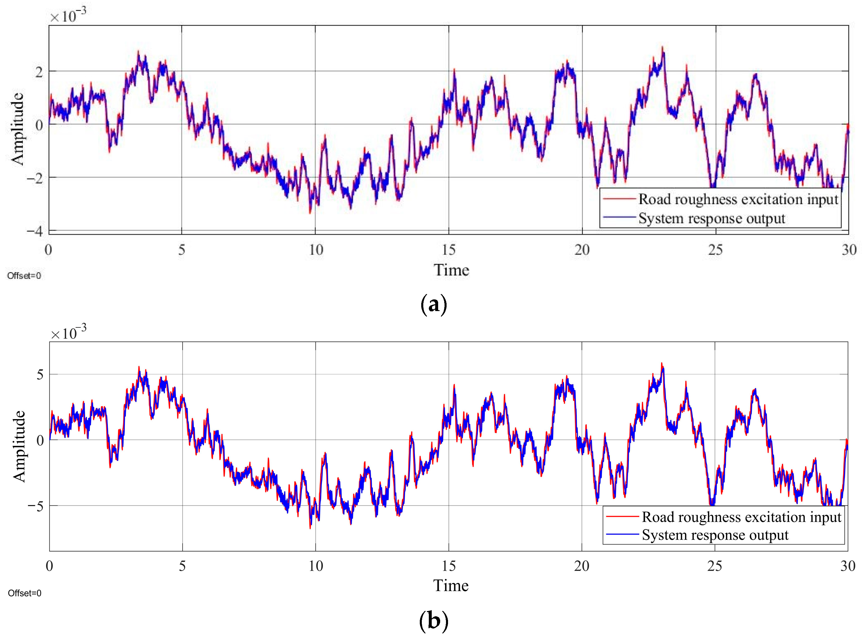
Figure 12 shows the responses of the hydraulic loading system with an electro-hydraulic proportional controller combined with a fuzzy PID control algorithm to input signals of random vibrations from Class B and C roads. The fuzzy PID control system exhibited a good response, with the output waveform being consistent with that of the input road vibrations. The relative errors in the simulation of the vibrations from Class B and C roads were 12.2% and 13.1%, respectively, which were both less than the 15% error required for engineering systems, confirming that the proposed fuzzy PID control system satisfied the requirements for practical engineering applications.
5. Conclusions
(1) A multi-functional compound simulation test bench was designed for the performance assessment of heavy vehicle hydropneumatic suspensions using the electro-hydraulic proportional control technique.
(2) A mathematical model was developed for describing the hydraulic loading system with electro-hydraulic proportional control, and the transfer function of the system was derived.
(3) Based on the established mathematical model of the electro-hydraulic proportional control hydraulic loading system, a Bode diagram was drawn using MATLAB 2018b software to analyze the stability of the system. A simulation model of the system was established in the Simulink environment to analyze its dynamic characteristics. The results showed that the hydraulic loading system with electro-hydraulic proportional control had good stability, smooth response, and no overshoot. However, the response was slow.
(4) The fuzzy control algorithm is added on the basis of the PID controller, and the fuzzy PID controller of the electro-hydraulic proportional system is established. The dynamic response characteristics of the hydraulic loading system with electro-hydraulic proportional control were improved. The improved system performed well in replicating the road vibrations from Class B and C roads.
(5) Due to time and funding constraints, this article was unable to complete the development and experimental work of an electro-hydraulic proportional control hydropneumatic suspension simulation test bench. Instead, it only analyzed the stability and dynamic characteristics of the system based on the established mathematical model. In the future, more experimental verification work will be carried out on this basis.
Author Contributions
Conceptualization, Z.W. and Y.Z.; methodology, Z.W. and Y.Z.; software, C.S.; validation, B.J., C.S. and H.Z.; formal analysis, B.J.; investigation, Z.W.; resources, B.J.; data curation, B.J. and C.S.; writing—original draft preparation, Z.W.; writing—review and editing, Z.W.; visualization, Y.Z.; supervision, Z.W.; project administration, Z.W.; funding acquisition, Z.W. All authors have read and agreed to the published version of the manuscript.
Funding
This research was funded by the Fund for Guiding the Transformation of Scientific and Technological Achievements of Shanxi Province, grant number 2021104021301061, and by the Fund for Fundamental Research Program of Shanxi Province, grant number 202203021221106.
Data Availability Statement
Not applicable.
Conflicts of Interest
The authors declare no conflict of interest.
References
- Wolfgang, B. Hydropneumatic Suspension Systems; Springer: Berlin, Germany, 2022. [Google Scholar] [CrossRef]
- Sohail, A.; Liu, C. Study on the vibration isolation characteristics of an anti-resonant hydropneumatic suspension. J. Eng. 2019, 13, 208–210. [Google Scholar] [CrossRef]
- Xia, X.; Meng, Z.; Han, X.; Li, H.; Tsukiji, T.; Xu, R.; Zheng, Z.; Ma, J. An Automated Driving Systems Data Acquisition and Analytics Platform. Transp. Res. Part C Emerg. Technol. 2023, 151, 104120. [Google Scholar] [CrossRef]
- Xia, X.; Hashemi, E.; Xiong, L.; Khajepour, A. Autonomous Vehicle Kinematics and Dynamics Synthesis for Sideslip Angle Estimation Based on Consensus Kalman Filter. IEEE Trans. Control Syst. Technol. 2023, 31, 179–192. [Google Scholar] [CrossRef]
- Liu, W.; Xia, X.; Xiong, L.; Lu, Y.; Gao, L.; Yu, Z. Automated Vehicle Sideslip Angle Estimation Considering Signal Measurement Characteristic. IEEE Sens. J. 2021, 21, 21675–21687. [Google Scholar] [CrossRef]
- Solomon, U.; Padmanabhan, C. Hydro-gas suspension system for a tracked vehicle: Modeling and analysis. J. Terramech. 2011, 48, 125–137. [Google Scholar] [CrossRef]
- Qin, B.; Zeng, R.; Li, X.; Yang, J. Design and performance analysis of the hydropneumatic suspension system for a novel road-rail vehicle. Appl. Sci. 2021, 11, 2221. [Google Scholar] [CrossRef]
- Zhang, Z.; Cao, S.; Ruan, C. Statistical linearization analysis of a hydropneumatic suspension system with nonlinearity. IEEE Access. 2018, 6, 73760–73773. [Google Scholar] [CrossRef]
- Bai, X.; Lu, L.; Sun, M.; Zhao, L.; Li, H. Research on Hydro-pneumatic Suspension Test Bench Based on Electro-hydraulic Proportional Control. Int. J. Fluid Power. 2023, 24, 537–566. [Google Scholar] [CrossRef]
- Luan, Z.; Sun, J.; Yang, Q. Research of controllable load module analysis and control algorithm on linear motor test platform. In Proceedings of the 2011 International Conference on Electric Information and Control Engineering, Wuhan, China, 15–17 April 2011; pp. 647–650. [Google Scholar] [CrossRef]
- Kulkarni, P.; Sawant, P.; Kulkarni, V. Design and Development of Plane Bending Fatigue Testing Machine for Composite Material. Mater. Today Proc. 2018, 5, 11563–11568. [Google Scholar] [CrossRef]
- Gao, Y. Design and Control of Electro-hydraulic Servo Active Suspension Road Simulation System. Master’s Thesis, Jilin University, Changchun, China, 2018. [Google Scholar]
- Wang, B. Research on Reproduction Methods of Road Roughness Using Road Simulator. Doctor’s Thesis, Wuhan University of Technology, Wuhan, China, 2010. [Google Scholar]
- Li, X. Research on Hydraulic Servo Control System for Automobile Shock Absorber Test-Bench. Master’s Thesis, Liaoning University of Technology, Jinzhou, China, 2016. [Google Scholar]
- Chen, X.; Wang, W.; Yang, Y.; Liu, Y.; Chen, X. Analysis and Design of a Vertical Loading Test Rig for Independent Suspension with Adjustable Hard Points. Automot. Eng. 2017, 39, 689–697. [Google Scholar] [CrossRef]
- Yang, J. Suspension K&C Characteristic Sensitivity Analysis to Automotive Handling. Master’s Thesis, Jilin University, Changchun, China, 2008. [Google Scholar]
- Si, Y. Design and Application Research of Suspension Matching Test Bench. Master’s Thesis, Xihua University, Chengdu, China, 2016. [Google Scholar]
- Zhao, Q.; Qin, Y.; Sun, Z.; Wang, N. Simulation Research on the Electro-hydraulic Servo Suspension Test Bench. For. Eng. 2020, 36, 60–682. [Google Scholar] [CrossRef]
- Qin, Y. Road Spectrum Reproduction and Suspension Control Based on Electro-hydraulic Servo System. Master’s Thesis, Northeast Forestry University, Harbin, China, 2020. [Google Scholar]
- Liu, G.; Gao, J.; Nie, G.; Fang, T.; Wang, X. Simulation of Suspension Testbed Based on Fuzzy-PID Control. Agric. Equip. Veh. Eng. 2015, 53, 51–55. [Google Scholar]
- Du, S.; Wu, Y.; Liu, M.; Liu, Z.; Lu, Q. Research on Road Simulation Test-Bed of Passenger Car Suspension System. Automot. Digest. 2020, 6, 49–52. [Google Scholar] [CrossRef]
- Zhan, H. Study on Control Methods for Electro-hydraulic Servo Loading System of Vehicle Hydro-pneumatic Suspension. Doctor’s Thesis, Harbin Institute of Technology, Harbin, China, 2012. [Google Scholar]
- Xu, G.; Luo, Y.; Yang, Y.; Zhang, J. New wheel ground simulation load model and system for vehicle dynamic performancetest. J. Instrum. 2018, 39, 214–223. [Google Scholar] [CrossRef]
- Liu, G.; Chen, S.; Wang, W.; Zhao, Y. Simulation and experimental research of a novel hydro-pneumatic suspension based on AMEsim and simulink. J. Vib. Meas. Diagn. 2016, 36, 346–350. [Google Scholar] [CrossRef]
- Li, B. Analysis and Experimental Research of Proportional Valve with Displacement Feedback by the Moving Valve Sleeve. Master’s Thesis, Zhejiang University, Hangzhou, China, 2013. [Google Scholar]
- GB/T 7031-2005; Mechanical Vibration Road Surface Spectrum Measurement Data Report. National Mechanical vibration and shock Standardization Technical Committee: Beijing, China, 2006.
- JT/T 448-2021; Automotive Suspension Device Testing Platform. National Automobile Maintenance Standardisation Technical Committee: Beijing, China, 2021.
- QC/T491-2018; Performance Requirements and Bench Test Methods for Automotive Shock Absorbers. National Automobile Standardization Technical Committee: Beijing, China, 2018.
- GB1589-2004; Boundary Dimensions, Axle Load, and Mass Limits for Road Vehicles. Ministry of Industry and Information Technology: Beijing, China, 2004.
- Lu, Z.; Zhang, J.; Xu, B.; Wang, D.; Su, Q.; Qian, J.; Yang, P.; Pan, M. Deadzone compensation control based on detection of micro flow rate in pilot stage of proportional directional valve. ISA Trans. 2019, 94, 234–245. [Google Scholar] [CrossRef] [PubMed]
- Zheng, K.; Chen, S. Nonlinear Modeling and Simulation of Asymmetric Hydraulic Cylinder Systems Controlled By Proportional Valves. Hydraul. Pneum. 2013, 4, 25–29. [Google Scholar] [CrossRef]
- Wu, Y.; Jiang, T.; Lu, Q.; Xia, C.; Fu, J.; Wang, Y.; Wu, Z. Characteristics of Thermally Actuated Pneumatic Proportional Pressure Valves and Their Application. J. Inst. Eng. Ser. C 2020, 101, 631–641. [Google Scholar] [CrossRef]
- Zhao, W.; Li, L. A New K-DOPs Collision Detection Algorithms Improved by GA. In Proceedings of the International Conference on Wireless Communications and Applications, Huangshan, China, 25 October 2012. [Google Scholar]
- Liu, B.; Qiang, B.; Quan, H. Modeling and Simulation of Electrohydraulic Proportional Position Control System. Hydraul. Pneum. Seal. 2011, 31, 45–49. [Google Scholar] [CrossRef]
- Xiao, Z.; Xing, J.; Peng, L. Further Study of Load Flow and Load Pressure. Mach. Tool Hydraul. 2007, 35, 130–133. [Google Scholar] [CrossRef]
- Wang, L. Simulation Study on Hydraulic Proportional Adjustment Control of Coal Mining Machinery. Master’s Thesis, Anhui University of Science and Technology, Huainan, China, 2019. [Google Scholar]
- Li, M.; Ren, G. Research on Electro-Hydraulic Proportional Self-Tuning Fuzzy-PID Control System Based on MATLAB. Appl. Mech. Mater. 2013, 423–426, 2882–2885. [Google Scholar] [CrossRef]
- Yu, Z. Automotive Theory, 5th ed.; China Machine Press: Beijing, China, 2009. [Google Scholar]
Figure 1.
Mechanical platform of simulation test bench. (a) Hydropneumatic suspension performance analysis; (b) 1/4 vehicle road simulations.
Figure 1.
Mechanical platform of simulation test bench. (a) Hydropneumatic suspension performance analysis; (b) 1/4 vehicle road simulations.
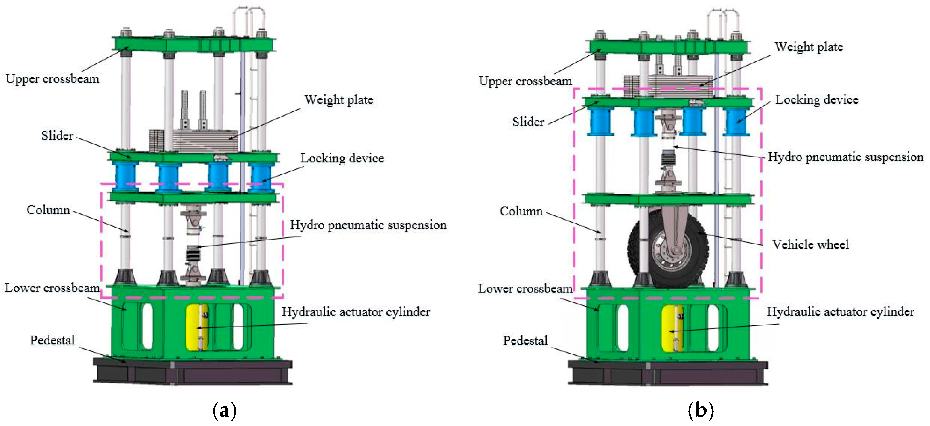
Figure 2.
Schematic diagram of the hydraulic loading system with electro-hydraulic proportional control. Key: 1: oil tank, 2: hydraulic pump and electric motor, 3: relief valves, 4: pressure gauges, 5: filters, 6: hydraulic check valves, 7: accumulator, 8: directional control valves (8-1 manual, 8-2 electro-hydraulic), 9: pilot hydraulic control check valves, 10: hydraulic cylinder.
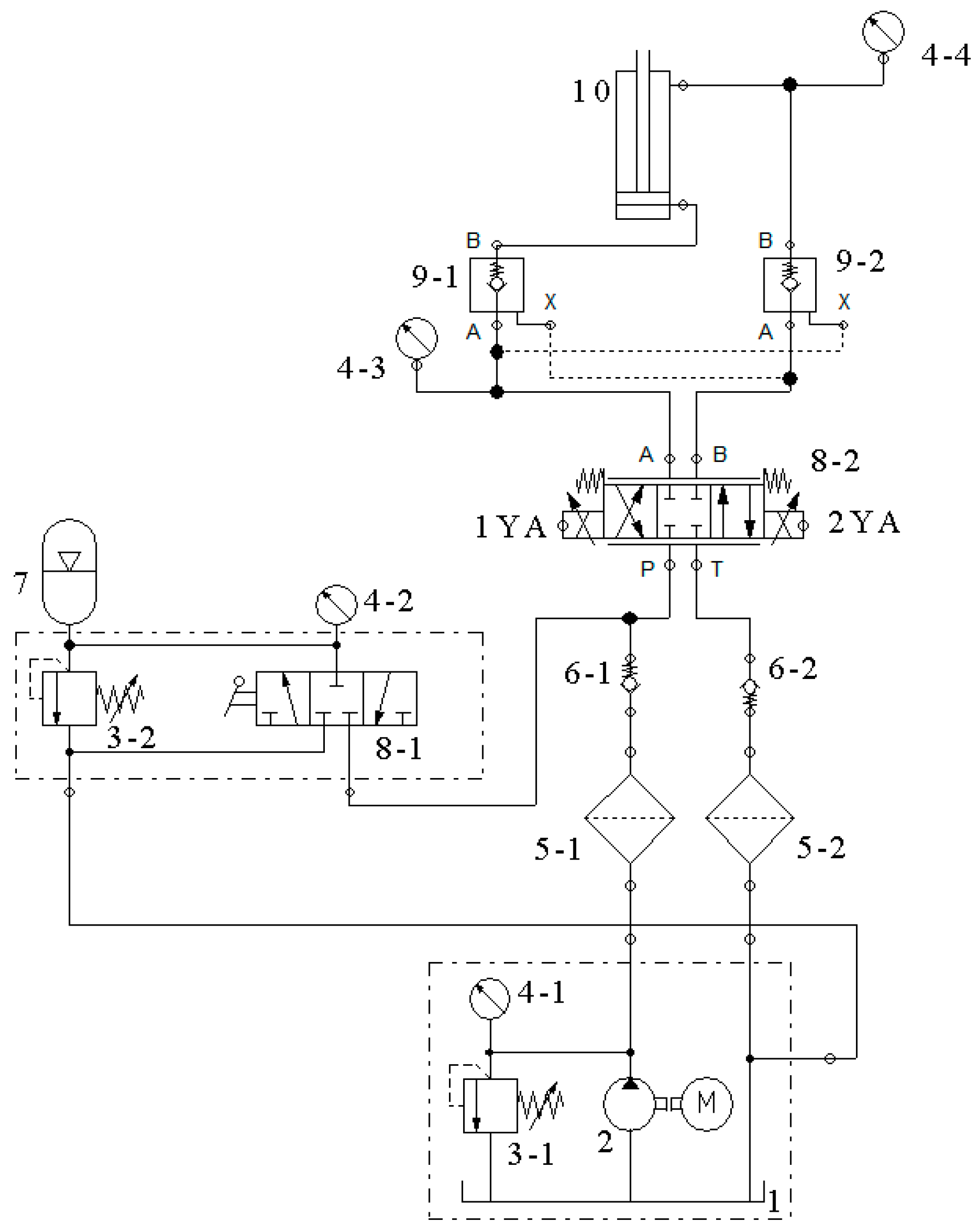
Figure 3.
Block diagram of electro-hydraulic proportional control system.
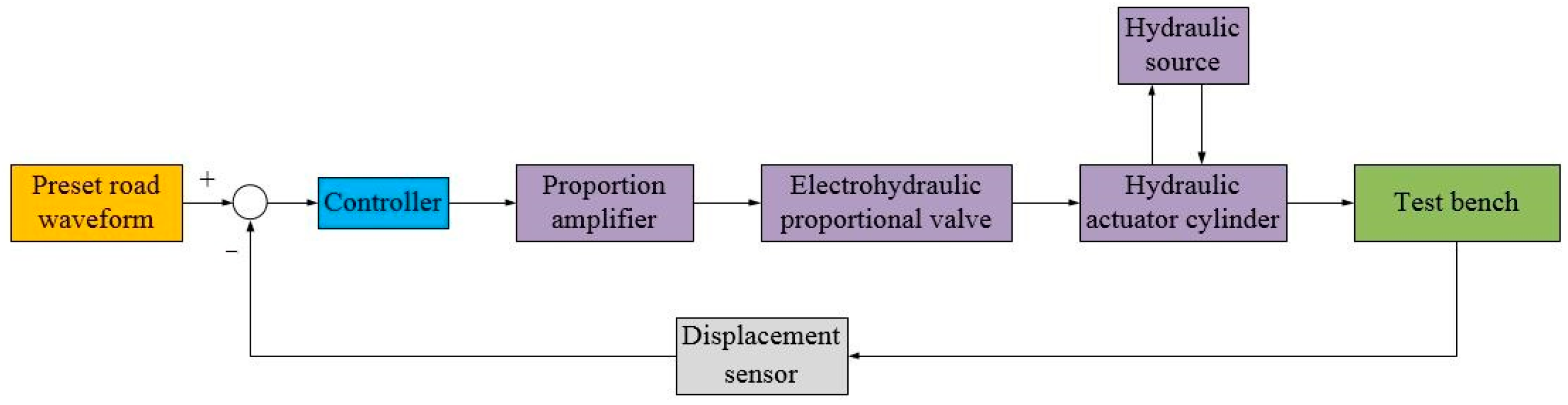
Figure 4.
Schematic diagram of valve-controlled hydraulic cylinder.
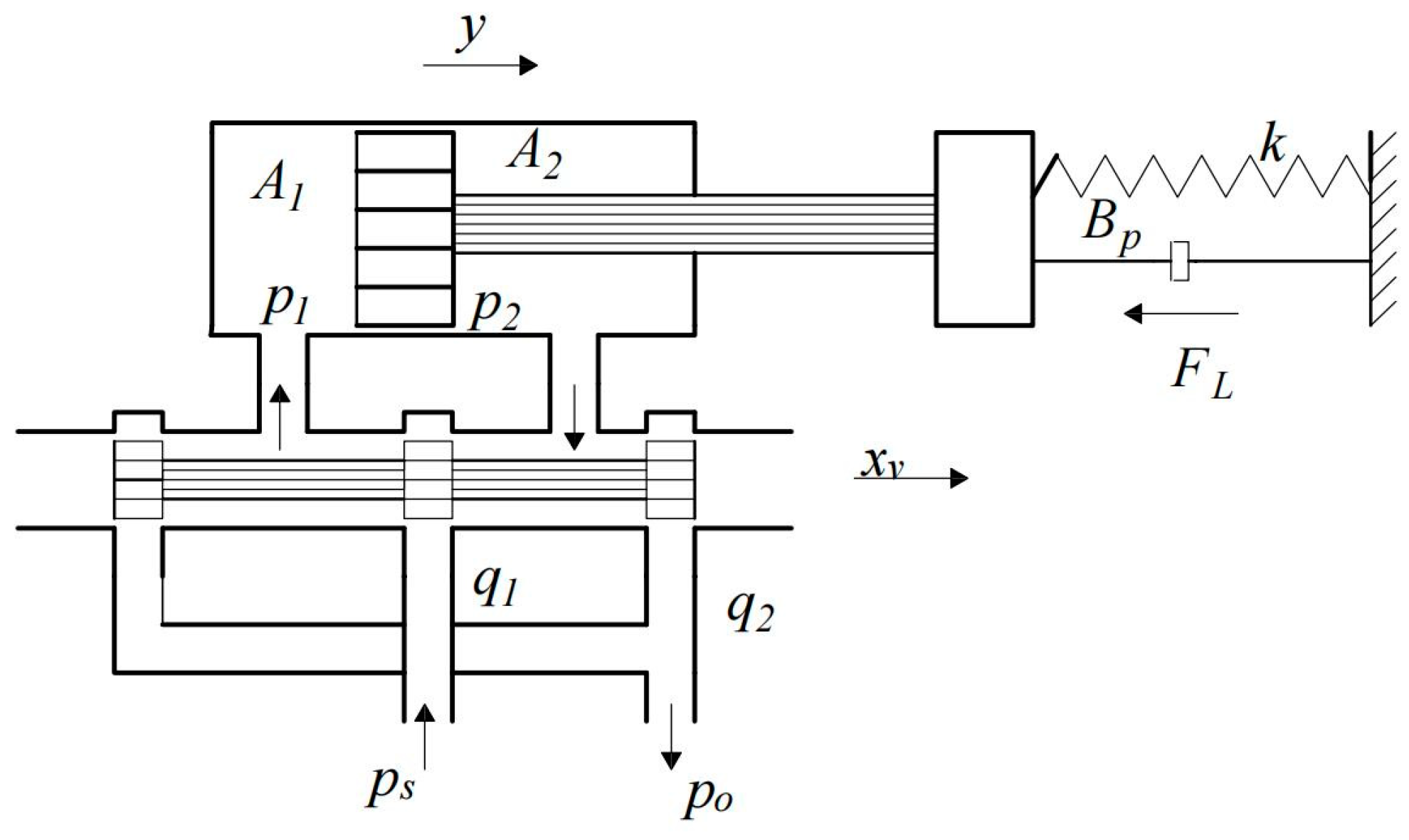
Figure 5.
Block diagram of the transfer functions of the control system.

Figure 6.
Open-loop Bode diagram of hydraulic loading system with electro-hydraulic proportional control.
Figure 6.
Open-loop Bode diagram of hydraulic loading system with electro-hydraulic proportional control.
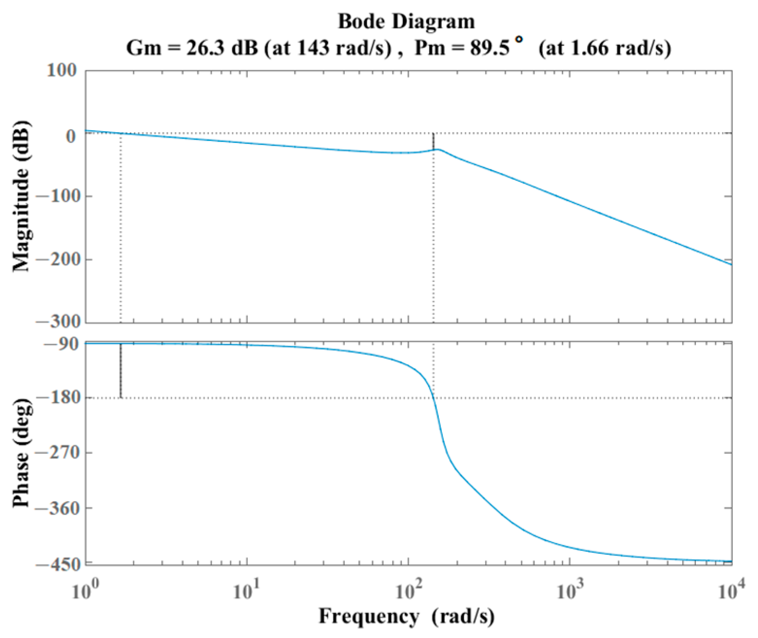
Figure 7.
Response curve of system to step input signal.

Figure 8.
Response curves of the system to sine signals: (a) 1 Hz, (b) 10 Hz, and (c) 25 Hz.
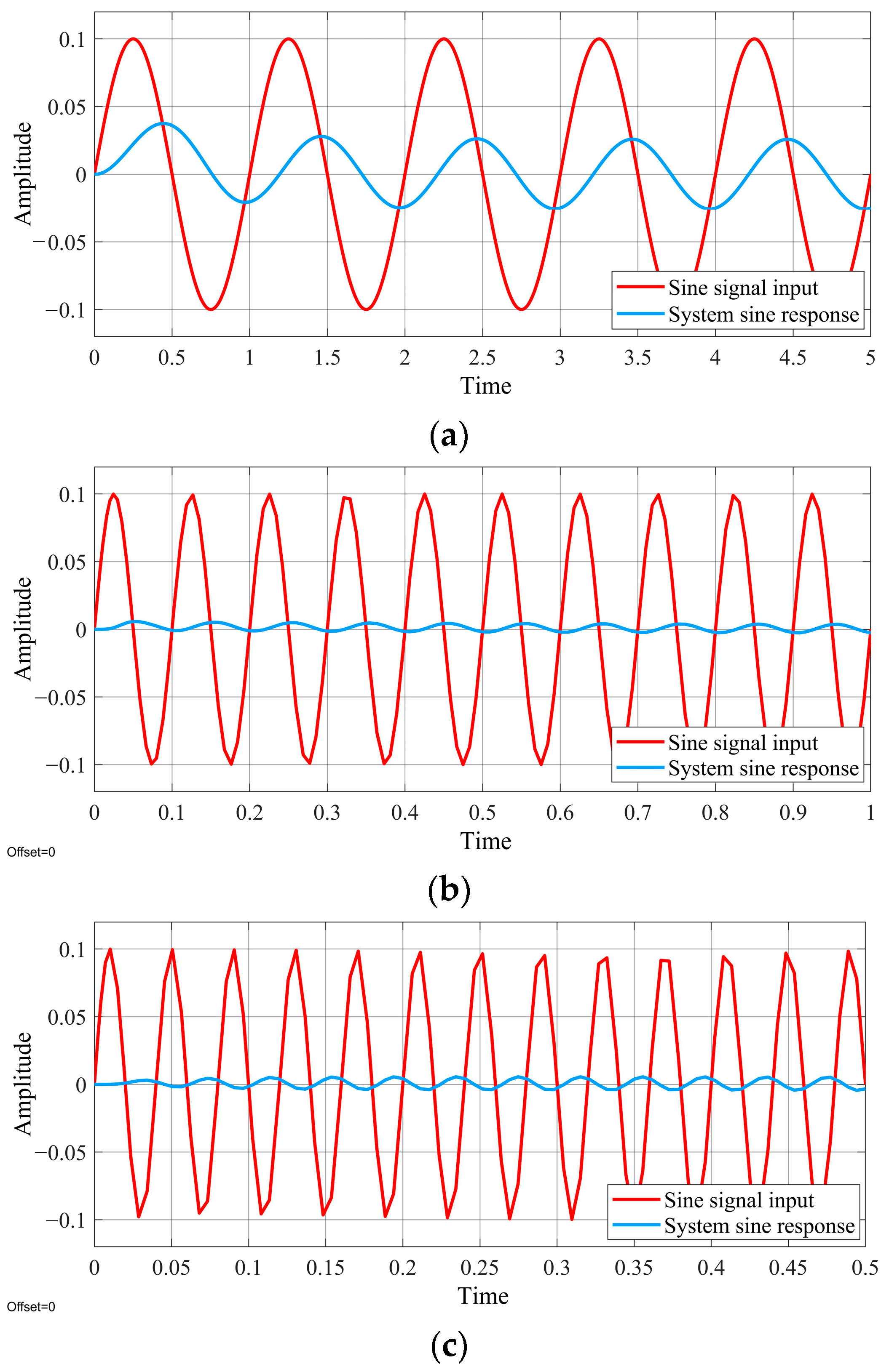
Figure 9.
Response curve to a step signal of the hydraulic loading system with an electro-hydraulic proportional controller combined with an adaptive fuzzy PID control algorithm.
Figure 9.
Response curve to a step signal of the hydraulic loading system with an electro-hydraulic proportional controller combined with an adaptive fuzzy PID control algorithm.
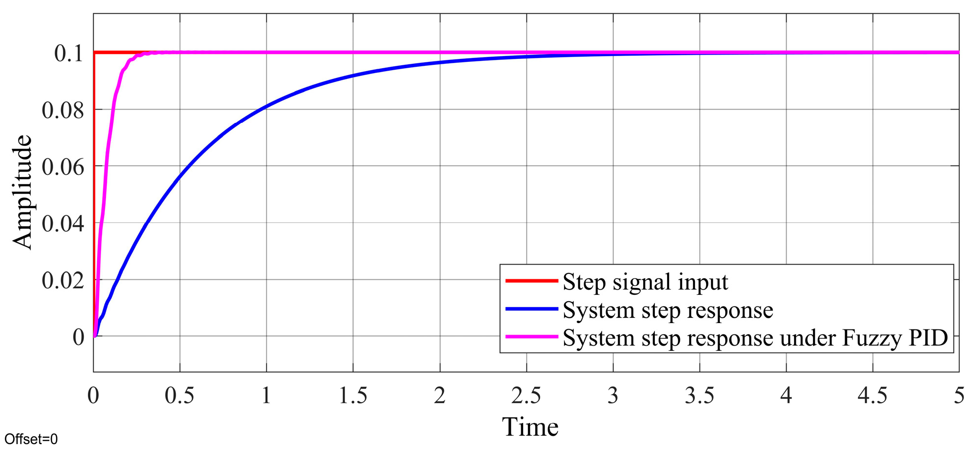
Figure 10.
Response curves to sine signals of different frequencies of the hydraulic loading system with an electro-hydraulic proportional controller incorporated with an adaptive fuzzy PID control algorithm: (a) 1 Hz, (b) 10 Hz, and (c) 25 Hz.
Figure 10.
Response curves to sine signals of different frequencies of the hydraulic loading system with an electro-hydraulic proportional controller incorporated with an adaptive fuzzy PID control algorithm: (a) 1 Hz, (b) 10 Hz, and (c) 25 Hz.
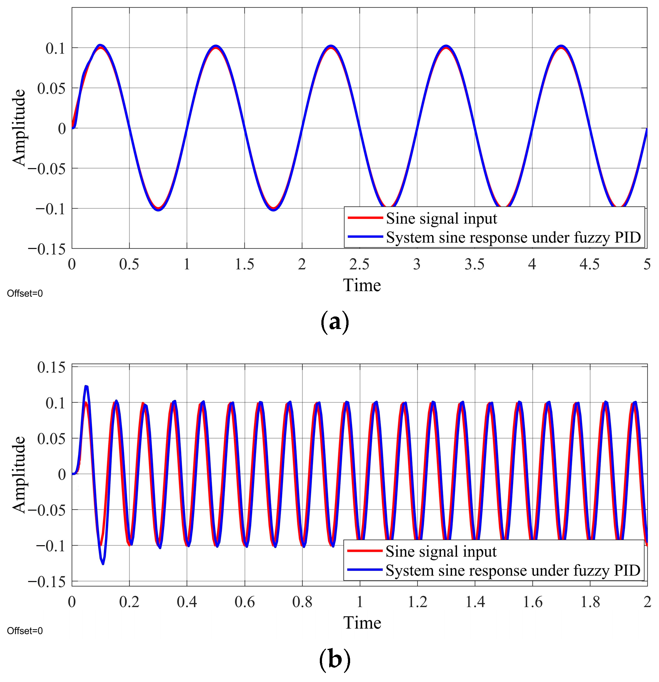

Figure 11.
Waveforms of road vibrations from Class B and C roads.
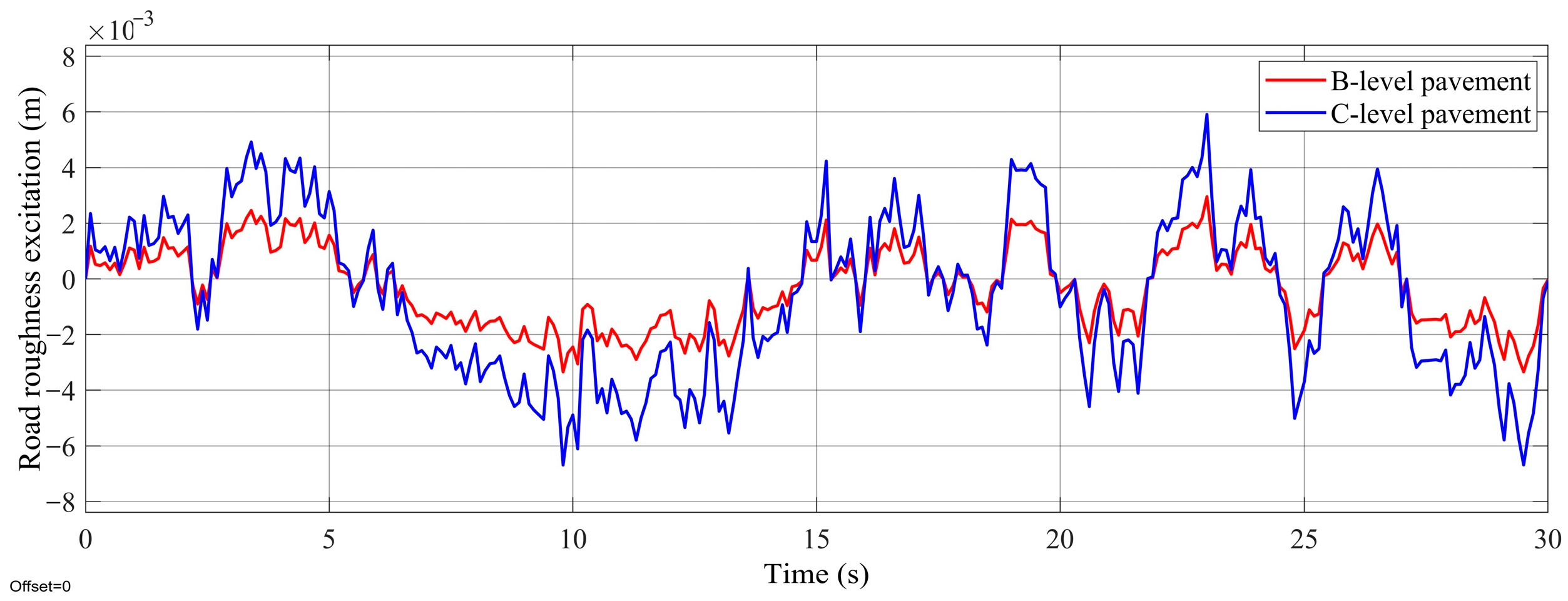
Figure 12.
Response curves to random road vibrations: (a) Class B roads, and (b) Class C roads.

Table 1.
Hydraulic cylinder dimensions and performance parameters.
| Maximum Stroke | Piston Diameter (d1) | Piston Rod Diameter (d2) | Rated Pressure | Maximum Pressure |
|---|---|---|---|---|
| ±120 mm | 125 mm | 60 mm | 6 MPa | 15 MPa |
Table 2.
Hydraulic pump parameters.
| Displacement | Maximum Speed | Rated Power | Rated Pressure | Maximum Pressure |
|---|---|---|---|---|
| 250 mL/r | 1450 rpm | 45 kW | 35 MPa | 40 MPa |
Table 3.
Parameters of electro-hydraulic proportional valve.
| Valve Weight | Rated Flow | Maximum Flow | Drift Diameter | Current Control Signal | Maximum Pressure |
|---|---|---|---|---|---|
| 11.5 kg | 300 L/min | 450 L/min | 16 mm | 4–20 mA | 31.5 MPa |
Table 4.
Major parameters of the hydraulic loading system with electro-hydraulic proportional control.
Table 4.
Major parameters of the hydraulic loading system with electro-hydraulic proportional control.
| Summary | Parameter | Summary | Parameter |
|---|---|---|---|
| Proportional amplifier gain (Ka) | 0.2 V/A | Hydraulic oil elastic modulus (βe) | 7 × 10⁸ Pa |
| Proportional valve gain (Ksv) | 0.09 m3/(s·A) | Proportional valve flow gain (Kq) | 0.05 m2/s |
| Proportional valve damping ratio (ζsv) | 0.6 | Displacement sensor gain (Kd) | 1 V/m |
| Natural frequency of proportional valve (ωsv) | 314 rad/s | Equivalent total mass of piston (mt) | 5100 kg |
| Effective area of piston cavity (A1) | 1.23 × 10⁻² m2 | Natural frequency of hydraulic system (ωp) | 154.42 rad/s |
| Effective area of rod cavity (A2) | 9.44 × 10⁻³ m2 | Damping ratio of hydraulic system (ζp) | 0.111 |
| Total volume of hydraulic cylinder (V) | 3.07 × 10⁻³ m3 | Internal leakage coefficient (Cip) | 3.3 × 10⁻³ m5/(N·s) |
| Initial volume of two chambers (V10/V20) | 3.74 × 10⁻⁴ m3 | External leakage coefficient (Cep) | 0 |
| Hydraulic spring stiffness (Ky) | 1.22 × 10⁸ N/m | Equivalent leakage coefficient (Cie) | 3.61 × 10⁻¹¹ m5/(N·s) |
| System flow coefficient (Kce) | 3.76 × 10⁻¹¹ | Additional leakage coefficient (Cf) | −2.81 × 10⁻¹² m5/(N·s) |
Table 5.
Fuzzy inference rules.
| △Kp/△Ki/△Kd | Ec | |||||||
|---|---|---|---|---|---|---|---|---|
| NB | NM | NS | ZO | PS | PM | PB | ||
| E | NB | PB/NB/PS | PB/NB/NS | PM/NM/NB | PM/NM/NB | PS/NS/NB | ZO/ZO/NM | ZO/ZP/PS |
| NM | PB/NB/PS | PB/NB/NS | PM/NM/NB | PS/NS/NM | PS/NS/NM | ZO/ZO/NS | NS/ZO/ZO | |
| NS | PM/NB/ZO | PM/NM/NS | PM/NS/NM | PS/NS/NM | ZO/ZO/NS | NS/PS/NS | NS/PS/ZO | |
| ZO | PM/NM/ZO | PM/NM/NS | ZS/NS/NS | ZO/ZO/NS | NS/PS/NS | NM/PM/NS | NM/PM/ZO | |
| PS | PS/NM/ZO | PS/NS/ZO | ZO/ZO/ZO | NS/PS/ZO | NS/PS/ZO | NM/PM/ZO | NM/PB/ZO | |
| PM | PS/ZO/PB | ZO/ZO/NS | NS/PS/PS | NM/PS/PS | NM/PM/PS | NM/PB/PS | NB/PB/PB | |
| PB | ZO/ZO/PB | ZO/ZO/PM | NM/PS/PM | NM/PM/PM | NM/PM/PS | NB/PB/PS | NB/PB/PB | |
Table 6.
Road roughness-based road classification.
| Road Classification | Road Roughness Coefficient (10−6 m3) | ||
| Lower Limit | Geometric Average | Upper Limit | |
| A | 8 | 16 | 32 |
| B | 32 | 64 | 128 |
| C | 128 | 256 | 512 |
| D | 512 | 1024 | 2048 |
| E | 2048 | 4096 | 8192 |
| F | 8192 | 16,384 | 32,768 |
| G | 32,768 | 65,536 | 131,072 |
| H | 131,072 | 262,144 | 524,288 |
Disclaimer/Publisher’s Note: The statements, opinions and data contained in all publications are solely those of the individual author(s) and contributor(s) and not of MDPI and/or the editor(s). MDPI and/or the editor(s) disclaim responsibility for any injury to people or property resulting from any ideas, methods, instructions or products referred to in the content. |
© 2023 by the authors. Licensee MDPI, Basel, Switzerland. This article is an open access article distributed under the terms and conditions of the Creative Commons Attribution (CC BY) license (https://creativecommons.org/licenses/by/4.0/).
Share and Cite
MDPI and ACS Style
Wu, Z.; Jiao, B.; Sun, C.; Zhang, Y.; Zhao, H. Design and Optimization of Hydropneumatic Suspension Simulation Test Bench with Electro-Hydraulic Proportional Control. Machines 2023, 11, 907. https://doi.org/10.3390/machines11090907
AMA Style
Wu Z, Jiao B, Sun C, Zhang Y, Zhao H. Design and Optimization of Hydropneumatic Suspension Simulation Test Bench with Electro-Hydraulic Proportional Control. Machines. 2023; 11(9):907. https://doi.org/10.3390/machines11090907
Chicago/Turabian StyleWu, Zhibo, Bin Jiao, Chuanmeng Sun, Yanbing Zhang, and Heming Zhao. 2023. "Design and Optimization of Hydropneumatic Suspension Simulation Test Bench with Electro-Hydraulic Proportional Control" Machines 11, no. 9: 907. https://doi.org/10.3390/machines11090907
Note that from the first issue of 2016, this journal uses article numbers instead of page numbers. See further details here.