
Design and Analysis of a Moment of Inertia Adjustment Device
1
Key Laboratory of Conveyance and Equipment, Ministry of Education, East China Jiaotong University, Nanchang 330013, China
2
Life-Cycle Technology Innovation Center of Intelligent Transportation Equipment, Nanchang 330013, China
*
Author to whom correspondence should be addressed.
Machines 2024, 12(3), 204; https://doi.org/10.3390/machines12030204
Submission received: 19 February 2024
/
Revised: 15 March 2024
/
Accepted: 19 March 2024
/
Published: 20 March 2024
(This article belongs to the Section Machine Design and Theory)
Abstract
:The vibration frequency characteristics of a rotor system are directly related to its moment of inertia. In this paper, a moment of inertia adjustment device is proposed to adjust the frequency characteristics of a rotor system and better reduce vibration by changing the moment of inertia. First, a mathematical model of the moment of inertia and the temperature field are established. A finite element simulation model of the electromagnetic field of the electromagnetic control unit in the device is established. The influence of current and air gap on the electromagnetic forces is discussed. Then, the validity of the finite element simulation for the electromagnetic control unit is verified using experimental results. In addition, the variations in the displacement and force of the moving mass and the moment of inertia of the device with speed are analyzed. The results show that the proposed moment of inertia adjustment device can be used to significantly adjust the moment of inertia, which provides a reference for better controlling vibrations in rotor systems. Finally, a finite element simulation model for an electromagnetic field analysis of the electromagnetic control unit in the device is established. The results show that the maximum temperature of the electromagnetic control device is 332 K in 60 min, which is in accordance with the requirements.
1. Introduction
A flywheel is a common mechanical device that is usually applied for alleviating speed fluctuations, energy storage, or suppressing vibration in machines [1,2]. Due to its high efficiency, low pollution, simple maintenance, etc., it is widely applied in advanced technical fields, including aerospace, vehicles, and energy engineering [3,4,5,6]. In order to achieve small fluctuations in angular velocity, a flywheel with a large moment of inertia is required. However, a large moment of inertia can make it difficult to start an engine or other rotor systems [7]. In general, the vibrations and speed fluctuations of a mechanical system become more severe as the speed increases. A variable inertia flywheel is a device that can effectively solve this problem, because the vibration frequency characteristics of a rotor system are directly related to its moment of inertia. Ref. [8] proposed a new semi-active electromagnetic device that can suppress automotive suspension vibration by controlling its inertia and damping. To achieve the vibration control of two DOF primary systems, a variable inertia vibration absorber was designed by Megahed [9]. Li et al. [10] designed a variable damping and inertia device that is installed in the vehicle suspension. Simulation results demonstrated that the device can achieve much better performances than the conventional structure. Researchers have conducted extensive research on variable inertia flywheels. Oliver [11] proposed a variable inertia flywheel, dividing the flywheel into two chambers with electrolytic fluid. The inertia of the flywheel is changed using a solenoid pump to move the electrolytic fluid from one chamber to another. Dugas [12] acquired variable inertia through the valve’s control over the fluid flow.
The above method for achieving variable moments of inertia involves changing the mass of the flywheel. But the actual structure implemented in this way will be very complex and difficult to operate. The research on the variable inertia flywheel mainly focuses on changing the distance from the movable mass in the flywheel to the center of rotation. A two-terminal mass-based vibration absorber with a variable moment of inertia achieved through the motions of sliders embedded in a hydraulic-driven flywheel for passive vehicle suspension was developed by Xu et al. [13]. Kondoh et al. [14] proposed a new type of flywheel energy storage system in which the moment of inertia is controlled actively for charging and discharging without a power electronic interface while the rotational speed is held almost constant. Concerning a hydraulic drive, a comparative study has been conducted on the effects of the variable inertia flywheel on the hydraulic motor speed fluctuations compared with those of the fixed inertia flywheel in the literature [15]. The results showed that the variable inertia generated by the variable inertia flywheel can better reduce the hydraulic motor speed fluctuations in response to the changes in the excitation inputs. A novel vibration absorber based on the variable inertia flywheel using magnetorheological fluid was proposed by Dong [16]. A new concept of an elastic flywheel using vulcanized rubber based on the principle of material strain was presented by Harrowell [17]. Recently, a vibration energy harvester for bicycles based on a directional variable inertia flywheel and coaxial mechanical motion rectifier was proposed by Chen et al. [18]. A flywheel with symmetrically placed mass spring dampers in a ballscrew-based power take-off system was presented by Li [19]. With its variable inertia and mass amplification effect, the system equivalent mass and corresponding parameters can be adapted using small mass spring dampers.
The moment of inertia of a rotor system directly affects its natural frequency characteristics, vibration characteristics, and transmission performance [20]. And the technology of variable moments of inertia has a high potential to reduce torque and speed fluctuations in mechanical systems. But until now, very few articles have reported on the application of variable inertia based on electromagnetic control. To reduce the vibration of seat suspension, an electromagnetic variable stiffness device that has a low energy consumption and energy harvesting capability was proposed by Ning [21]. Researchers like Peter Ibrahim have designed electromagnetic vibration energy harvesters with a tunable mass moment of inertia [22]. The resonance frequency of this type of device can be adjusted to match that of the excitation. Li et al. designed a magneto-rheological variable stiffness and damping torsional vibration absorber that can reduce the angular displacement fluctuations in experimental setup [23]. A novel electromagnetic variable inertance device was designed for vehicle vibration reduction in ref. [24]. There is a need to explore the realization of variable moments of inertia based on electromagnetic control. In this work, an electromagnetic control unit was introduced. Thus, a new type of easily detachable moment of inertia adjustment device is proposed. A finite element simulation analysis of the electromagnetic field and temperature field characteristics of the electromagnetic control unit was conducted, and the results were verified through experiments.
2. The Structure and Working Principle of the Moment of Inertia Adjustment Device
Figure 1 shows the structure of the moment of inertia adjustment device, which mainly consists of a frame and three electromagnetic control units. The frame is a regular triangular prism with through holes in the center of the shaft and threaded holes in the sides and ends. And the electromagnetic control unit is composed of two permanent magnets, a coil, a spring, a sleeve, and a cylinder. The coil is wound around permanent magnet 1 and fixed in the cylinder with adhesive. Permanent magnet 2 was fixed in the sleeve using adhesive. The sleeve and the frame are connected by the spring. Besides that, the two permanent magnets are installed in the cylinder with the same poles opposite each other. The cylinder is then attached to the frame with screws. When the device rotates, the radial position of permanent magnet 2 and the sleeve can be adjusted by changing the coil current under the actions of centrifugal force, spring force, and electromagnetic force. In this way, different moments of inertia can be obtained.
3. Theoretical Analysis of the Moment of Inertia Adjustment Device
3.1. Mathematical Model of Moment of Inertia
When the moment of inertia adjustment device works, permanent magnet 2 and the sleeve can slide along the cylinder. Since electromagnetic control units installed on the moment of inertia adjustment device are evenly arranged relative to the rotational center, a mechanical analysis of the permanent magnet 2 and sleeve in a single electromagnetic control unit was conducted. As shown in Figure 2a, point O is the rotational center. Permanent magnet 2 and the sleeve are regarded as a whole part (as one moving mass), and the mass is set to be m. The stiffness and initial length of the spring are k and l0, respectively. The distance from the spring to point O is r0, and the distance from the center of the moving mass to point O is r.
The centrifugal force Fc of the moving mass is
where ω is the rotational angular velocity.
As shown in Figure 2b, when the centroid of the moving mass is below the center of the device, the gravity of the moving mass will enhance the centrifugal force; however, when the centroid of the mass is above the center of the device, it weakens the centrifugal force. The component force Fm of gravity in the direction of the centrifugal force is
where g is the gravity acceleration, and t is the operating time of the device.
The friction Ff of the moving mass is
where μ is the Coulomb friction factor, and Fn is normal force on the friction surface.
When the spring deformation is Δl, the force Fs on the moving mass is
During the movement of the moving mass, the air gap δ has the following relationship with the spring deflecton Δl:
The length l of the spring after deflection under forces is
The distance r from the center of the moving mass to point O is
After the speed of the device has stabilized, the following equation is obtained according to the force balance on the moving mass:
It is assumed that the relationship between the electromagnetic force and the air gap under the specific current of the coil conforms to the following formula [25]:
where C1, C2, and C3 are constants, and the air gap δ is expressed in meters.
Fm is a sinusoidal function of high-frequency oscillations, i.e., the effect of gravity on the centrifugal force is a high-frequency signal that varies alternately in positive and negative equal amplitudes. The maximum value of this force is 3 N. Compared with the centrifugal force, the influence of the gravity of the moving mass is negligible, so the computational model is simplified. From Equations (1)–(9), the following equation can be obtained:
According to the parallel axis theorem, the moment of inertia of a single permanent magnet 2 and sleeve around the rotational center can be expressed as follows [7]:
where d2 is the diameter of the sleeve, and h2 is the height of the sleeve.
There are three sets of electromagnetic control units. Thus, the total moment of inertia can be expressed as follows [26]:
where Ju is the inertia expression of the immutable part in the structure.
3.2. Mathematical Model of Temperature Field
The coils in the electromagnetic control unit are direct current coils, which generate heat from the resistive losses caused by the passage of current through the conductor. The eddy current losses in the coils as well as in the small gaps between coils are neglected, and it is assumed that all electrical energy losses in the coil area are converted into heat. Referring to the result in ref. [27], the values of the following parameters need to be obtained. The heating power P of coils is expressed as follows:
where I is the coil current; R is the resistance of the coil; and ρ is the wire resistivity of the coil. l and s are the length and cross-sectional area of the wire, respectively.
Normally, the thermal conductivity of materials varies with temperature. To simplify the simulation process, the thermal conductivity of the material is assumed to be constant over a certain temperature range. The composite heat transfer coefficient hs between the stationary electromagnetic control unit and the environment is
where hc is the natural convection heat transfer coefficient, and hr is the radiative heat transfer coefficient.
When the device rotates, the heat transfer coefficient ha of the electromagnetic control unit positively depends on the average air flow speed, since the electromagnetic control unit is influenced by tangential and axial air flows [27]:
where vt is the average airflow velocity at the surface of the electromagnetic control unit.
4. Electromagnetic Field Simulation of the Moment of Inertia Adjustment Device
4.1. Electromagnetic Field Simulation Analysis
The finite element simulation software COMSOL Multiphysics 5.5 was used to analyze the electromagnetic force characteristics and magnetic induction distribution of the moment of inertia adjustment device. A two-dimensional axisymmetric model of the electromagnetic control unit was established, as shown in Figure 3. The frame was made of 6061 aluminum alloy, a non-magnetic material, and was not taken into account. The two permanent magnets were all made of a strong neodymium–iron–boron magnet. The material of the coil is copper. The other parts were the air shed. The dimensions of all the elements included in the model are listed in Table 1. The characteristic parameters of the finite element analysis are listed in Table 2.
The residual magnet model was selected to be under Ampere’s law option for permanent magnets, and parameters such as coil current I and coil turns N were set. As shown in Figure 4, triangle elements were used to divide the grid. For the area between the coil and permanent magnet 1, the boundary layer option was used to encrypt the grid. The maximum and minimum sizes of the grid element were 3.6 mm and 0.01 mm, respectively. Permanent magnet 2 and the sleeve, which are moving parts, were set to move radially. The initial position (air gap) relative to permanent magnet 1 was δ0 = 20 mm.
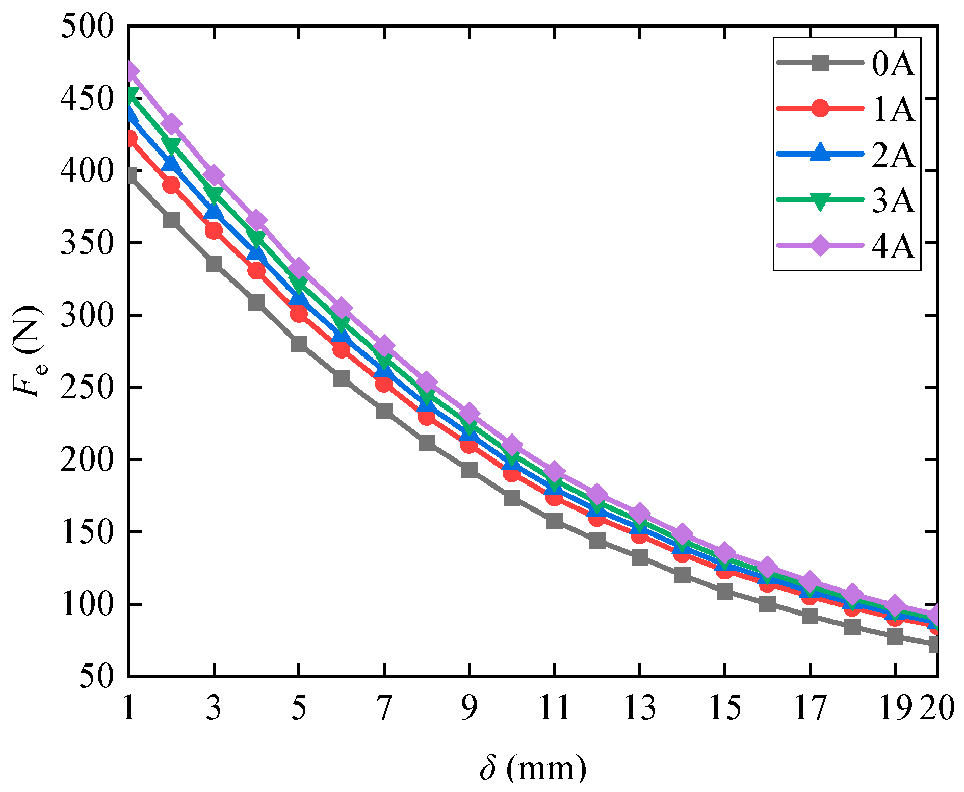
Given I = 0 A, 1 A, 2 A, 3 A, and 4 A, respectively, the electromagnetic field finite element simulation was conducted. Figure 5 shows the magnetic field line distribution and the magnetic induction intensity cloud diagram of the electromagnetic control unit for the current of 2 A. It can be seen that the magnetic field lines start from the N pole of the permanent magnet, pass through air, and return to the S pole of the permanent magnet to form a closed loop. The magnetic fields of the two permanent magnets are in opposite directions. In addition, the magnetic induction intensity on a permanent magnet exhibits characteristics of being large at both ends and small in the middle, with a relatively uniform distribution. The maximum value appears at the point where the structural shape changes. Because the magnetic field lines of the permanent magnet converge from the two poles, resulting in an increase in the magnetic induction intensity at both ends of the permanent magnet. Due to the strongest interaction between the magnetic field of the permanent magnet and the magnetic field generated by the coil at the intersection of permanent magnet 1 and the coil, the magnetic field of the permanent magnet and the magnetic field generated by the coil have the strongest superposition effect.
Figure 6 shows the relationship between the electromagnetic force Fe of the electromagnetic control unit with air gap under different currents. At a constant current value, the electromagnetic force decreases as the air gap increases. In addition, when the size of the air gap is in the range of 1–10 mm, the tendency of the electromagnetic force to change with the air gap is more obvious and the curve trend is steeper, while the opposite is true when the size of the air gap δ is in the range of 10–20 mm. The larger the air gap, the smaller the electromagnetic force due to the large magnetoresistance of air, which attenuates greatly as the magnetic lines of force pass through it.
4.2. Electromagnetic Force Test
To verify the validity of the finite element model and simulation analysis results, an electromagnetic force test system was constructed, as shown in Figure 7. Permanent magnet 2 and permanent magnet 1 with coil were fixed to the base with a support. The gap (air gap δ) between the two permanent magnets could be controlled by adjusting the distance between the supports. The input current of the coil in the electromagnetic control units could be changed using an adjustable DC power supply, and the electromagnetic force acting on permanent magnet 2 was input to a computer through a force sensor, digital transmitter, and USB-485 serial cable.
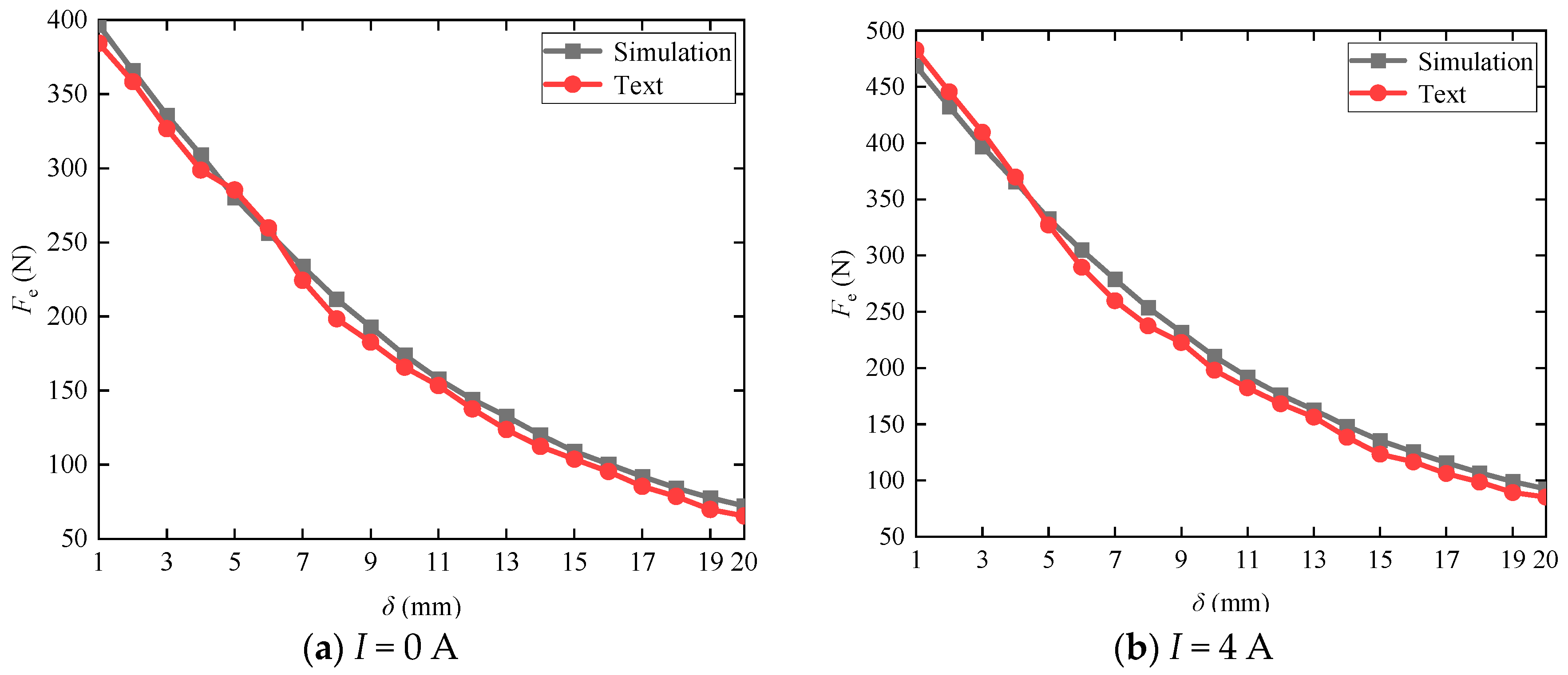
The electromagnetic force that acts on permanent magnet 2 under different air gaps was tested when the coil current was 0 A and 4 A. Figure 8 shows the comparison between the electromagnetic force test results and the simulation analysis results. Under the same conditions, the variation in electromagnetic force with air gap obtained from the test was close to that of the simulation results. Due to the existence of influencing factors such as part processing, the test environment, geometric model simplification in the finite element analysis, grid size, and solution accuracy, there were some differences between the actual electromagnetic force obtained from the test and the simulation results. The maximum relative error between them was 7.33%, which demonstrates that the finite element simulation model of the electromagnetic field and analysis results for the electromagnetic control unit are effective.
4.3. Calculation of the Moment of Inertia
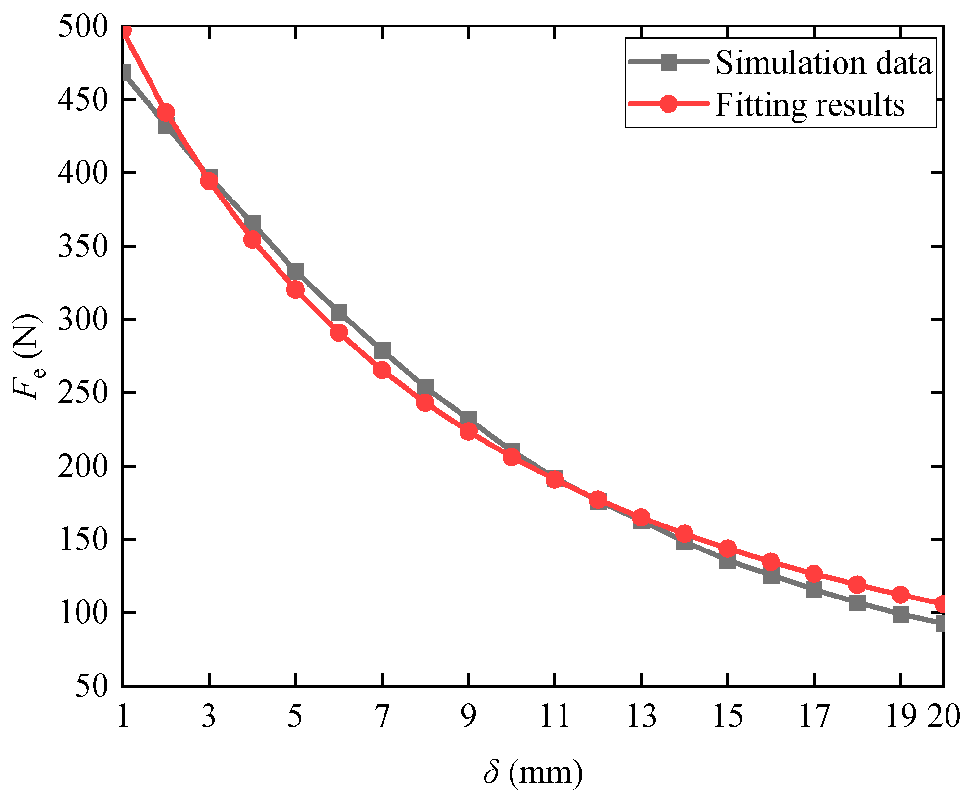
Based on Equation (7), nonlinear fitting was performed on the data for the finite element simulation analysis of the electromagnetic force when coil current I = 4 A, as shown in Figure 9. In this condition, C1 = 0.1319, C2 = 0.01529, and C3 = 0.
In the electromagnetic control unit, the mass of the moving mass was m = 0.3 kg, the stiffness of the spring was k = 15 N/mm, r0 = 35 mm, l0 = 26 mm, and the original inertia expression of the immutable part was Ju = 0.006 kg·m2. According to the analysis based on MATLAB R2021b, the relationship between the moment of inertia of the device and the rotation speed could be obtained when the input current of the coil was taken to be 0 A, 2 A, and 4 A, as shown in Figure 10.
As the rotation speed increases, the moment of inertia of the structure also increases. Until the moving mass reaches the limit position, the moment of inertia remains unchanged as the rotation speed continues to increase. However, the minimum value of the moment of inertia is different for different currents. The main reason for this is that the electromagnetic force on the moving mass is different even at a speed of 0 r/min for different currents, and therefore, the spring deformation Δl is also different. As the speed increases, the influence of the current on the moment of inertia becomes stronger, because at low speeds, the influence of the current on the electromagnetic force is small. In addition, the minimum and maximum moments of inertia of the structure were 0.01178 kg·m2 and 0.01638 kg·m2, respectively. The maximum adjustable proportion of its moment of inertia was 39.04%.
5. Temperature Field Simulation of the Moment of Inertia Adjustment Device
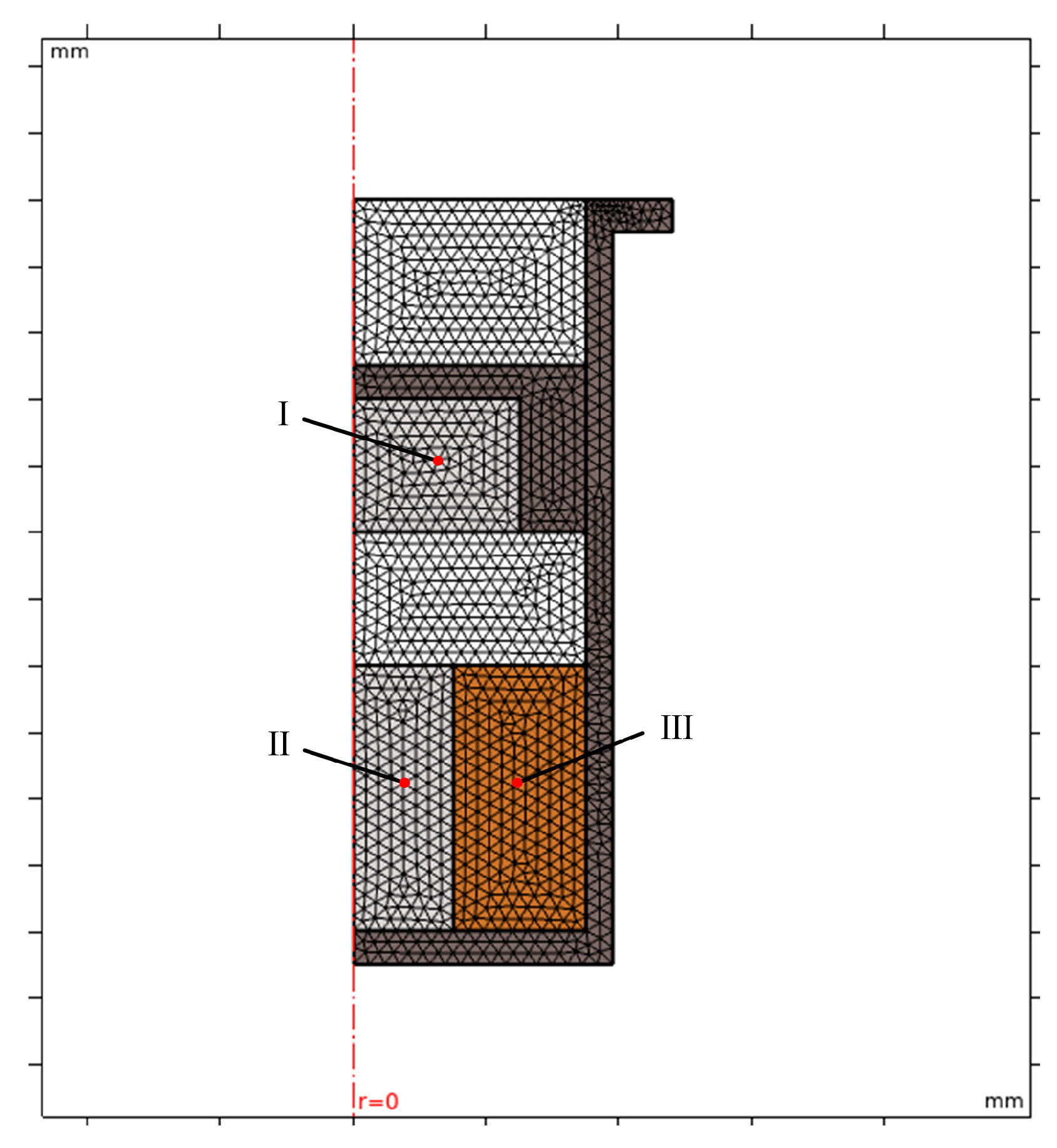
Heat transfer occurs when there is contact between two objects and there is a temperature difference. The temperature field transient simulation of the electromagnetic control unit was carried out using finite element software. In order to improve the accuracy and computational efficiency of the solution of the temperature field, several approximate processing methods and assumptions were proposed. First, the contact between parts within the electromagnetic control unit was relatively close, so the thermal contact resistance was ignored in the thermal simulation. Second, some editing processes were ignored, and non-essential model structures were minimized to facilitate meshing. Finally, the heating power of the coil was uniform. A finite element model of the electromagnetic control unit is shown in Figure 11. The maximum and minimum sizes of the grid element were 1.2 mm and 0.008 mm, respectively. Point I (the center of permanent magnet 2), point II (the center of permanent magnet 1), and point III (the center of the coil) were selected at different positions to analyze the temperature changes.
The initial ambient temperature was set to 293 K, and the rotational speed of the electromagnetic control unit was set to 2000 r/min. The operating current and time were set to 4 A and 60 min, respectively, and the rest of the parameters and parameter values are listed in Table 3.
A temperature distribution cloud diagram of the electromagnetic control unit is shown in Figure 12. The coil was located between permanent magnet 1 and the cylinder, and the internal heat transfer method of the electromagnetic control unit was solid thermal conduction, so the temperature here was the highest.
Figure 13 shows the variation in the temperature at different positions over time. The temperature of the electromagnetic control unit increased with time and then stabilized. And the maximum temperature of the coil and permanent magnet 1 was 322 K. Because the thermal conductivity of neodymium–iron–boron is lower than that of copper, the temperature of permanent magnet 1 was slightly lower than the temperature of the coil. In addition, the coil was in direct contact with permanent magnet 1, and there was air between the coil and permanent magnet 2, so the temperature of permanent magnet 2 changed more slowly than that of permanent magnet 1.
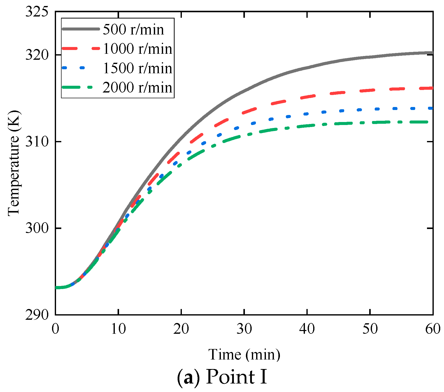
The temperature field simulation was carried out by varying the rotational speed to 500 r/min, 1000 r/min, and 1500 r/min. Figure 14 presents the variation in the temperature of point I, point II, and point III with time at different rotational speeds. The temperature rose over time and then stabilized. In addition, in the first 10 min, the rotational speed increased while the temperature remained almost constant as it takes time for the heat to be transferred from the coil to the surface. Then, the temperature decreased as the rotational speed increased. The most susceptible component to temperature influences is the neodymium–iron–boron magnet in the electromagnetic control unit, which has a maximum operating temperature of 350 K. During the whole process, the maximum temperature of the permanent magnet was 332 K, which is consistent with the requirements. The maximum operating temperature of the coil was 358 K. In addition, the maximum temperature at point III was 332 K, which is consistent with the requirements.
6. Conclusions
This study contributed the following:
- (1)
- A moment of inertia adjustment device was proposed that analyzes the forces acting on a moving mass while the device is rotating and takes into account gravity, friction, centrifugal force, spring force, and electromagnetic force. The forces acting on the moving mass while the device is rotating were analyzed by considering gravity, friction, centrifugal force, spring force, and electromagnetic force at the same time, and a computational model of the device was established. Compared with the centrifugal force, the influence of the gravity of the moving mass is negligible, so the computational model was simplified. The results show that r is related to the rotational angular velocity ω and the electromagnetic force Fe. Therefore, the control of r can be realized by adjusting Fe. The mathematical model of the moment of inertia was established, and the relationship between the moment of inertia and r was obtained. The results show that the control of the moment of inertia can be achieved by adjusting r. A temperature field model was established to obtain some parameter values for use in the simulation software.
- (2)
- A electromagnetic field simulation model for the electromagnetic control device was established. The following assumptions were made for the electromagnetic field calculations. First, the magnetic induction was assumed to be uniformly distributed in the magnetic field. Second, leakage from the coil and permanent magnet was neglected. The distribution characteristics of the electromagnetic field and the variation in electromagnetic force with air gap were analyzed. The results show that at a constant current value, the electromagnetic force decreases as the air gap increases. When the air gap is constant, the electromagnetic force increases with increasing current. An electromagnetic force test system of the electromagnetic control unit was designed and constructed. The results of the electromagnetic force test are close to the results of the finite element simulation analysis, which confirms the accuracy and effectiveness of the simulation model. The maximum relative error between them was 7.33%. The variation in the device’s moment of inertia under different speeds and currents was discussed. The results show that the proposed moment of inertia adjustment device can be used to significantly adjust the moment of inertia. The maximum adjustable proportion of its moment of inertia can reach 39.04%. This work provides a reference for better controlling vibrations in rotor systems.
- (3)
- A temperature field simulation model for the electromagnetic control device was established. The following assumptions were made for the temperature field calculations. First, the coil heating power was assumed to be uniform. Second, the contact resistance between parts was neglected. The temperature variation in the electromagnetic control device was analyzed. The temperature of the electromagnetic control unit increased with time and then stabilized. The temperature of permanent magnet 1 was slightly lower than the temperature of the coil, and both of their temperatures were higher than the temperature of permanent magnet 2. The results show that the maximum temperature of the electromagnetic control device was 332 K in 60 min, while the maximum operating temperatures of the permanent magnet and coil were 350 K and 358 K, respectively, which are in accordance with the requirements.
Author Contributions
Conceptualization, L.Z.; methodology, Z.W.; software, Z.W.; validation, Z.W.; formal analysis, G.L.; investigation, L.Z.; resources, L.Z.; data curation, Z.W.; writing—original draft preparation, Z.W.; writing—review and editing, L.Z.; supervision, G.L.; project administration, L.Z. All authors have read and agreed to the published version of the manuscript.
Funding
This work was supported by the National Natural Science Foundation of China (Grant Nos. 51805167 and 52265011), the Natural Science Foundation of Jiangxi Province (Grant No. 20232BAB204044), and the Foundation of Educational Department of Jiangxi Province (Grant No. GJJ2200624).
Data Availability Statement
The raw data required to reproduce these findings cannot be shared easily due to technical limitations (some files are too large). However, the authors can share the data upon any individual request (please contact the corresponding author through their mailing address).
Conflicts of Interest
The authors declare no conflicts of interest.
References
- Ge, Z.; Li, G.; Chen, S.; Wang, W. Influence of Nonlinear Characteristics of Planetary Flywheel Inerter Actuator on Vehicle Active Suspension Performance. Actuators 2023, 12, 252. [Google Scholar] [CrossRef]
- Christopher, D.A.; Beach, R. Flywheel technology development program for aerospace applications. IEEE Aerosp. Electron. Syst. Mag. 1998, 13, 9–14. [Google Scholar] [CrossRef]
- Amiryar, M.E.; Pullen, K.R. Analysis of Standby Losses and Charging Cycles in Flywheel Energy Storage Systems. Energies 2020, 13, 4441. [Google Scholar] [CrossRef]
- Hu, H.; Wei, J.; Wang, H.; Xiao, P.; Zeng, Y.; Liu, K. Analysis of the Notch Filter Insertion Position for Natural Frequency Vibration Suppression in a Magnetic Suspended Flywheel Energy Storage System. Actuators 2023, 12, 22. [Google Scholar] [CrossRef]
- Bolund, B.; Bernhoff, H.; Leijon, M. Flywheel energy and power storage systems. Renew. Sustain. Energy Rev. 2007, 11, 235–258. [Google Scholar] [CrossRef]
- Li, T.; Zeng, F.; Qin, J. The determination of moment of inertia of flywheel for pulsed-load diesel generator. In Proceedings of the Second International Conference on Mechanic Automation & Control Engineering, Mongolia, China, 15–17 July 2011; IEEE: Piscataway, NJ, USA, 2011. [Google Scholar]
- Yang, S.; Xu, T.; Li, C.; Liang, M.; Baddour, N. Design, Modeling and Testing of a Two-Terminal Mass Device With a Variable Inertia Flywheel. J. Mech. Des. 2016, 138, 095001. [Google Scholar] [CrossRef]
- Liu, P.; Ning, D.; Luo, L.; Zhang, N.; Du, H. An electromagnetic variable inertance and damping seat suspension with controllable circuits. IEEE Trans. Ind. Electron. 2021, 69, 2811–2821. [Google Scholar] [CrossRef]
- Megahed, S.M.; Abd El-Razik, A.K. Vibration control of two degrees of freedom system using variable inertia vibration absorbers: Modeling and simulation. J. Sound Vib. 2010, 329, 4841–4865. [Google Scholar] [CrossRef]
- Li, W.; Dong, X.; Yu, J.; Xi, J.; Pan, C. Vibration control of vehicle suspension with magneto-rheological variable damping and inertia. J. Intell. Mater. Syst. Struct. 2021, 32, 1484–1503. [Google Scholar] [CrossRef]
- Oliver, W.; Burstall, J. Variable Inertia Flywheel. U.S. Patent 20030178972A1, 26 April 2005. [Google Scholar]
- Dugas, P.J. Variable Inertia Flywheel. U.S. Patent US20150204418A1, 23 July 2015. [Google Scholar]
- Xu, T.; Liang, M.; Li, C. Design and analysis of a shock absorber with variable moment of inertia for passive vehicle suspensions. J. Sound Vib. 2015, 355, 66–85. [Google Scholar] [CrossRef]
- Kondoh, J.; Funamoto, T.; Nakanishi, T.; Arai, R. Energy characteristics of a fixed-speed flywheel energy storage system with direct grid-connection. Energy 2018, 165, 701–708. [Google Scholar] [CrossRef]
- Kushwaha, P.; Ghoshal, S.K.; Dasgupta, K. Dynamic analysis of a hydraulic motor drive with variable inertia flywheel. Proc. Inst. Mech. Eng. Part I J. Syst. Control Eng. 2019, 234, 734–747. [Google Scholar] [CrossRef]
- Dong, X.; Xi, J.; Chen, P. Magneto-rheological variable inertia flywheel. Smart Mater. Struct. 2018, 27, 115015. [Google Scholar] [CrossRef]
- Harrowell, R.V. Elastomer flywheel energy store. Int. J. Mech. Sci. 1994, 36, 95–103. [Google Scholar] [CrossRef]
- Chen, P.; Yang, Y. Design, Dynamics Modeling, and Experiments of a Vibration Energy Harvester on Bicycle. Trans. Mechatron. 2023, 28, 2670–2678. [Google Scholar] [CrossRef]
- Li, Q.; Li, X.; Mi, J. Tunable wave energy converter using variable inertia flywheel. IEEE Trans. Sustain. Energy 2020, 12, 1265–1274. [Google Scholar] [CrossRef]
- Luan, G.; Liu, P.; Ning, D.; Liu, G.; Du, H. Semi-Active Vibration Control of Seat Suspension Equipped with a Variable Equivalent Inertance-Variable Damping Device. Machines 2023, 11, 284. [Google Scholar] [CrossRef]
- Ning, D.; Du, H.; Sun, S.; Zheng, M.; Li, W.; Zhang, N.; Jia, Z. An electromagnetic variable stiffness device for semiactive seat suspension vibration control. IEEE Trans. Ind. Electron. 2019, 67, 6773–6784. [Google Scholar] [CrossRef]
- Ibrahim, P.; Arafa, M.; Anis, Y. An electromagnetic vibration energy harvester with a tunable mass moment of inertia. Sensors 2021, 21, 5611. [Google Scholar] [CrossRef] [PubMed]
- Li, W.; Dong, X.; Xi, J.; Deng, X.; Shi, K.; Zhou, Y. Semi-active vibration control of a transmission system using a magneto-rheological variable stiffness and damping torsional vibration absorber. Proc. Inst. Mech. Eng. Part D J. Automob. Eng. 2021, 235, 2679–2698. [Google Scholar] [CrossRef]
- Liu, P.; Zheng, M.; Ning, D.; Luo, L.; Zhang, N. A Novel Controllable Electromagnetic Variable Inertance Device for Vehicle Vibration Reduction. Vib. Eng. A Sustain. Future Act. Passiv. Noise Vib. Control. 2021, 1, 103–109. [Google Scholar]
- Chen, H.; Li, Y.; Long, Z.; Chang, W. Optimal design and characteristic analysis of hybrid magnet in maglev system. J. Syst. Simul. 2010, 22, 837–840. [Google Scholar]
- Zhang, Y.; Zhang, X.; Qian, T.; Hu, R. Modeling and simulation of a passive variable inertia flywheel for diesel generator. Energy Rep. 2020, 6, 58–68. [Google Scholar] [CrossRef]
- Wang, S.Y.; Song, W.L.; Li, H.L.; Wang, N. Modeling and multi-field simulation analysis of a multi-cylindrical magneto-rheological brake. Int. J. Appl. Electromagn. Mech. 2018, 57, 399–414. [Google Scholar] [CrossRef]
Figure 1.
Schematic of the structure of the moment of inertia adjustment device. 1—Cylinder; 2—Coil; 3—Permanent Magnet 1; 4—Permanent Magnet 2; 5—Sleeve; 6—Spring; 7—Frame.
Figure 1.
Schematic of the structure of the moment of inertia adjustment device. 1—Cylinder; 2—Coil; 3—Permanent Magnet 1; 4—Permanent Magnet 2; 5—Sleeve; 6—Spring; 7—Frame.

Figure 2.
Force analysis at different positions.


Figure 3.
A two-dimensional axisymmetric model of electromagnetic control devices.

Figure 4.
Grid division of finite element model.

Figure 5.
Magnetic force line distribution and magnetic induction intensity cloud diagrams.

Figure 6.
The variation in the electromagnetic force with air gap under different currents.

Figure 7.
Electromagnetic force test system for the electromagnetic device.

Figure 8.
Comparison between test results of electromagnetic force and finite element simulation.

Figure 9.
Nonlinear fitting of electromagnetic force simulation data when I = 4 A.

Figure 10.
The variation in moment of inertia with speed at different currents.

Figure 11.
Finite element modeling of electromagnetic control units.

Figure 12.
Temperature distribution cloud diagram of the electromagnetic control unit.

Figure 13.
The variation in the temperature at different positions over time.

Figure 14.
The variation in the temperature at different points with time at different rotational speeds.
Figure 14.
The variation in the temperature at different points with time at different rotational speeds.


Table 1.
The dimensions of all the elements included in the model.
| Parameter | Numerical Value | Parameter | Numerical Value |
|---|---|---|---|
| Permanent magnet 1 diameter d1 (mm) | 30 | Sleeve outside diameter d2 (mm) | 70 |
| Permanent magnet 2 diameter d3 (mm) | 50 | Cylinder outside diameter d4 (mm) | 78 |
| Permanent magnet 1 heights h1 (mm) | 40 | Permanent magnet 2 heights h3 (mm) | 20 |
| Sleeve heights h2 (mm) | 24 | Coil diameter d5 (mm) | 1 |
Table 2.
The characteristic parameters of the finite element analysis.
| Parameter | Numerical Value | Parameter | Numerical Value |
|---|---|---|---|
| Curie point of the permanent magnets (K) | 350 | Permanent magnet remanence Br (T) | 1.43 |
| Air permeability µ0 (H/mm) | 1.25 × 10⁻⁸ | Coercivity of permanent magnets (kA/mm) | 10.34 |
Table 3.
Main parameters of temperature field model.
| Parameter | Value |
|---|---|
| Heating power of the coil P (W) | 45.1 |
| Composite thermal conductivity hs (W/(m2·K)) | 9.7 |
| Thermal conductivity ha (W/(m2·K)) | 59.6 |
Disclaimer/Publisher’s Note: The statements, opinions and data contained in all publications are solely those of the individual author(s) and contributor(s) and not of MDPI and/or the editor(s). MDPI and/or the editor(s) disclaim responsibility for any injury to people or property resulting from any ideas, methods, instructions or products referred to in the content. |
© 2024 by the authors. Licensee MDPI, Basel, Switzerland. This article is an open access article distributed under the terms and conditions of the Creative Commons Attribution (CC BY) license (https://creativecommons.org/licenses/by/4.0/).
Share and Cite
MDPI and ACS Style
Zeng, L.; Wan, Z.; Li, G. Design and Analysis of a Moment of Inertia Adjustment Device. Machines 2024, 12, 204. https://doi.org/10.3390/machines12030204
AMA Style
Zeng L, Wan Z, Li G. Design and Analysis of a Moment of Inertia Adjustment Device. Machines. 2024; 12(3):204. https://doi.org/10.3390/machines12030204
Chicago/Turabian StyleZeng, Liping, Zihao Wan, and Gang Li. 2024. "Design and Analysis of a Moment of Inertia Adjustment Device" Machines 12, no. 3: 204. https://doi.org/10.3390/machines12030204
Note that from the first issue of 2016, this journal uses article numbers instead of page numbers. See further details here.