1. Introduction
Modern industrial plants are complex systems that need to run over several weeks or months. During a production run, operating conditions can change, which can lead to abnormal behavior of the process. Since modern plants’ control and measurement devices are strongly cross-linked with each other, a failure in a major piece of equipment can potentially lead to plant-wide disturbances and for example result in a flood of alarms, making it difficult to localize the root cause of the disturbance. As not all relations of the different process parameters are well known, data-driven methods can be of great help to localize or at least to narrow down on the cause of a disturbance.
Backtracking the disturbance propagation path using data-driven methods means to detect temporal cause-effect relationships in a data set. In detail, this means that statistical relationships and time-shifts are used to reconstruct the propagation direction of the disturbance. Several methods have been already developed to test for temporal causal dependencies in data:
One of the first approaches was made by Granger [
1], who compares two autoregressive models. The first model contains only past values of itself; the second model is augmented with past values of another variable. If the augmentation improves the regression, it is assumed that this variable has a causal impact on the other. In [
2], an algorithm for root cause localization based on the cross-correlation function is presented for causal analysis, especially when having valve stiction. Schreiber [
3] presents a concept, named transfer entropy, which detects causal dependencies by measuring the reduction of uncertainty when one variable predicts future values of the other. Further methods for the detection of causal dependencies are proposed in terms of dynamic Bayesian networks [
4,
5] or nearest neighbor approaches [
6]. An overview about different methods, tested on artificial benchmark data sets and for biosignal analysis, is given in [
7].
In this paper, different algorithms are proposed, which are based on the cross-correlation function, the transfer entropy, Granger causality and support vector machines. Next, the results of the different methods are combined, and a root cause priority list is generated. This priority list contains a ranking of the different process variables describing their possibility as being the actual cause of the fault.
All proposed algorithms consist of a statistical test, which determines whether the disturbance traveling from one process variable to a second is significant, and a quantitative part, called the causal strength, which defines the influence the input variable has on the output variable. For all methods, the causal strength takes values between zero(= no causal dependency) and one (= causal dependency). Finally, this value is used for generating the root cause priority list. The paper centralizes the main results given in [
8], containing the following main contributions: (1) a proposal of a new algorithm based on support vector machines by using a recursive variable selection and model reduction approach; (2) the development of a design approach to combine all methods into one causal matrix and transfer into a root cause priority list; (3) the extension of an existing method based on the cross-correlation function by using permutation tests for the significance test; and (4) the development of a visualization method for the causal matrices. The paper is structured as follows:
In
Section 2, the foundations for the detection of causal dependencies in dynamic systems are introduced.
Section 3 explains the algorithms. In
Section 4, it is pointed out how the results of the different methods can be combined and how the root cause priority list is calculated. Additionally, a new way to visualize the results from the different methods is described. Finally,
Section 5 tests the methods on data from a simulated chemical stirred-tank reactor and on an experimental laboratory plant.
2. Detecting Causal Dependencies in Process Measurements
Definition (causal system): A time-invariant system is causal if, for all input signals with and , for any , the output signals for show the characteristic (with : the initial state). Systems that are not causal are called acausal. In causal systems, the input signals for do not have an impact on the behavior of the output signal until time . Additionally, for causal systems, the impulse response for is zero.
This definition of causality results in several system theoretic consequences. For all static systems , causality exists, even if u or y is seen as the input signal, since in both cases, the output signal is not depending on future values, but on the current value of the input signal.
Additionally, all linear time-continuous systems with one input and one output signal are causal, since and explain the data equally well (: Laplace-transformed input and output signals). In that case, it is only possible to test if the transfer function is realizable (order of the numerator polynom ≤ order of the denominator polynom). Still, this does not contain information about causality.
To backtrack the disturbance propagation path in a plant, a signal decay time or a signal dead time needs to be present in the measurements. Decay times between and characterize a smoothing effect, so that seems to be delayed with respect to . A dead time between and exists, if does not depend on in , but only on in . In other words, dead times describe the interval a change in the input signal needs to become visible on the output of the system. In industrial processes dead times exist, e.g., in tubes, when measuring a fluid concentration on different positioned sensors.
Another point of view on causality is given by Pearl [
9]. The central idea is that a cause
C increases the probability of the appearance of an effect
E. This means that
C can only be the cause of
E, if
is fulfilled. However, an increase of the probability can only be done through an active intervention. Therefore, Pearl introduces the do-operator, which forces setting
C on a fixed value. In other words,
C only has a causal impact on
E, if
is fulfilled. This approach is the only possibility to avoid the detection of false causal dependencies.
An example for the detection of a false causal dependency is a non-measured signal
, which has an impact on
u, as well as a later one on
y, without having a direct dependency pointing from
u to
y. In [
10], it is shown how the approach given by Pearl can be used to detect causal structures in process data. Since the methods proposed in this paper only rely on observational data, meaning that no active intervention is performed, this approach will not be pursued in this paper.
3. Methods for Reconstructing the Disturbance Propagation Path
3.1. Cross-Correlation Function
The cross-correlation function (CCF) [
11] quantifies the linear similarity of two equidistant sampled time series
that are time-shifted by a constant lag
λ. The CCF is defined as:
with
and:
with
.
means that
and
are perfectly correlated at a shift
λ, while values close to zero indicate that there is no correlation.
3.1.1. Significance Test
To check for a significant cause-effect relationship , two tests are established. The first test is used to check if differs significantly from zero; the second test checks if the causal strength from differs significantly from to have a clear indication of the direction of the propagation path.
Significant time-shifted correlation: Since the available samples of the two time series are limited, Equation (
1) only gives an estimation of the CCF, so that
randomly differs from zero for two uncorrelated signals. To test if
differs significantly from zero, a hypothesis test is performed. We define:
If
holds, there could be a causal relation from
, and the hypothesis test is performed. To check if a significant correlation between the signals is present, a
t-test with the null hypothesis defined as having no correlation is used with significance level
. If this test fails, it is assumed that no cause-effect relationship exists from
.
Significant causal direction: This test covers the possibility that the resulting CCF can have a global maximum for
and a slightly lower local maximum for
, meaning that the causal direction is not obvious. Therefore, this test checks if the maximum for
is significantly different from the maximum for
. To perform the test, a compound parameter
defined as:
with
is used. A significance value
indicates a causal dependency from
. As
strongly depends on the characteristics of
and
, an adaptive threshold is derived through a
permutation test. Since performing a complete permutation of
destroys all causal information, the resulting value of
should be close to zero. This idea is exploited by calculating random permutations of
and generating several values for
. The threshold
for each pair of variables is calculated as:
with
being the mean value and
the standard deviation. If
holds, the test has passed successfully.
If both significance tests are passed, the found causal dependency is assumed to exist.
3.1.2. Causal Strength
The causal strength of
is defined as:
with
.
is a design parameter to make the different methods numerically compatible, and its selection will be explained in
Section 4. The proposed algorithm for the detection of cause-effect relationships for two time series
and
using the CCF is summarized as follows:
| Algorithm 1: Algorithm based on cross-correlation. |
Compute of and and determine ; If , then , else test for a significant correlation; Calculate and corresponding threshold ; Check if ; calculate the causal strength by
|
3.2. Granger Causality
The Granger causality (GC) has been introduced by Clive Granger [
1] and is traditionally used in the field of economics [
12,
13]. Recently, the application of GC is of growing interest, especially in the field of neuroscience [
14] and biology [
15].
The central idea is that it is assumed that a signal
has a causal influence on
if past values from
and
result in a better prediction of
than using only past values from
for prediction. GC takes into account that besides the signal
[k],
can depend on further signals
. A comparison is done using two vector autoregressive models and performing a one-step-ahead prediction. If the prediction error of the first model is substantially smaller than the one from the second model, a causal dependency
is concluded. For the proposed algorithm, each time series is once selected as output
, while the left
time series are used as input. This can be formulated with
n defining the model order as:
By definition, the parameters
,
in Equation (
7) and (8) result from separate estimations. The impact of the
i-th input signal is measured in terms of the sum of the squares of residuals without
as
and with
as
and is used to test for causal significance and for calculating the causal strength.
The performance of the model strongly depends on the model order
n. A too small of a value for
n leads to a large prediction error, and setting
n too large results in an overfitted model. Therefore, the Akaike information criterion (AIC) [
16] is used for model order estimation, while taking into account the prediction errors, the sample size
K, the number of variables
r and the model order
n. For model order estimation, the loss function is once set to
for the unrestricted and to
for the restricted model. The AIC is defined as:
while the estimated order is selected as
. Furthermore, all models are tested for consistency by performing a Durbin-Watson statistic [
17] on the residuals.
3.2.1. Significance Test
This test is performed to check whether
and
differ significantly. According to [
3,
and
follow
distributions, and an
F-test can be performed to verify if the time series
has a causal influence on
. The test is performed on the restricted and unrestricted model under the null hypothesis that
with significance level
.
3.2.2. Causal Strength
The strength of the significant causal relationship
is defined as:
with
, since
counts. The design parameter
will be determined in
Section 4. The suggested algorithm is summarized as follows:
| Algorithm 2: Algorithm based on Granger causality. |
Compute and using the model order estimated through AIC; Test for model consistency for both models using the Durbin–Watson statistic; Perform a significance test based on an F-test for ; If the causal dependency is significant, calculate the causal strength by ;
|
3.3. Transfer Entropy
The transfer entropy (TE) is an information theoretic measure and was first introduced by Schreiber [
18]. Applications of the TE can be found, e.g., in neuroscience [
19,
20] and in financial data analysis [
21]. In the field of process engineering, research has been conducted by Bauer [
6], who uses TE for the causal analysis of measurements taken from chemical processes.
From its definition, it can be used to detect causal dependencies by testing how much information is transferred from
to
and how much information is transferred from
to
. The transition probability for
is defined as
, which is used as short notation for:
with
n defining the time horizon and
} the quantization levels of
. The transition probability
is defined accordingly. The transfer entropy is then given as:
According to [
21], the boundaries of the TE are
, with
being the entropy of the output signal. To capture dead times in the data, the parameter
λ is introduced to perform a backward-shifting of
, and Equation (
12) is calculated for different
. For the calculation of causal dependencies, the maximum value of the transfer entropy is set to
. To calculate the value of the time horizon
n, the residual sum of squares of several vector autoregressive models is calculated:
with
resulting from a least squares estimation. The used order
is then chosen as the minimum of the Akaike information criterion defined as
[
16].
3.3.1. Significance Test
Testing for a significant causal relationship is done by a test introduced in [
3]. The key idea is to generate an adaptive threshold
based on the permutated input time series
and the generation of several values for
. The values of
are finally used to calculate the threshold
in terms of a
-test:
with mean value
and standard deviation
. If
holds, a causal dependency
is concluded, and the causal strength can be calculated.
3.3.2. Causal Strength
By definition
, meaning that for normalizing to values between zero and one, the causal strength of the transfer entropy can be defined as:
The design parameter
will be chosen in
Section 4. The suggested algorithm for the detection of cause-effect relations is summarized as:
| Algorithm 3: Algorithm based on transfer entropy. |
Compute model order of the transfer entropy using VAR models and AIC; Compute of the time series and , set ; Calculate and check if ; Set as the resulting value of the causal strength
|
3.4. Support Vector Machines for Regression
Support vector machines (SVM) are learning methods that are used for supervised learning. Originally, they were developed by Vapnik [
22] for classification and later on were extended towards regression and time series prediction [
23]. In industrial processes, they are used, e.g., for fault detection and diagnosis [
24] or optimization [
25]. For the detection of causal structures in data, a model reduction approach is proposed.
Given a training set with
with
and
, an SVR means to find the regression function:
containing as parameters the normal vector
w, the bias
b and
, denoting the scalar product. The function
should have at most a deviation
ϵ from the values
for the whole training data set, while seeking a normal vector
w, which is as small as possible. As the selection of a too small insensitivity zone
ϵ would lead to equations with infeasible constraints, slack variables
and an additional weighting parameter
are introduced leading to the objective function:
The optimization problem is solved by means of its dual containing the Lagrange multipliers
. The solutions of the regression function is finally given by:
Kernel functions: One of the main reasons why SVMs are employed is their ability to deal with nonlinear dependencies by introducing so-called kernel functions; see, e.g., [
26,
27]. The input data
is mapped into some feature space
with a possibly higher dimension by using a nonlinear transformation function Φ and searching for the flattest function in the defined feature space. Since SVMs solely depend on the calculation of dot products, the computational complexity for this transformation remainsfeasible. A kernel function, defined as
, can be plugged into Equation (
18), resulting in the final regression function:
In this paper, only Gaussian kernels, defined as
, are used for the detection of causal structures. To optimize the parameters
and
σ, a downhill simplex algorithm [
28] is used.
3.4.1. Detecting Causal Dependencies
To detect cause-effect dependencies, an input data set
for predicting
is generated. The SVM is once trained and optimized regarding
and
σ on the complete data set. The time horizon
n is estimated as given in Equation (
13) for the transfer entropy.
To detect cause-effect dependencies, an input data set
for predicting
is generated. The SVM is once trained and optimized regarding
and
σ on the complete data set. The time horizon
n is estimated as given in Equation (
13).
In the first step, the variables in
are ranked in terms of their prediction accuracy of
by performing a recursive variable elimination algorithm based on the Lagrange multipliers as proposed by [
29].
In the second step, a relevant subset of input variables is selected. If the resulting subset contains one or several past values of
, it is assumed that
u causes
y. For the selection of the size of the subset, an
F-test [
11] (
) is performed on the resulting residual sum of squares of the two SVMs, while the first SVM contains
ψ variables and the second SVM
variables. If the null hypothesis cannot be rejected, the residual sum of squares does not change significantly, and the found subset of variables is set to size
ψ.
3.4.2. Causal Strength
Similar to Granger causality, the causal strength is calculated based on the comparison of the squared sum of residuals. The causal strength is calculated through a comparison of the two different squared sums of residuals, named and , while . In detail, is calculated using the above explained SVM with the subset of input variables resulting from the initial set . For the prediction of , the residual sum of squares is calculated by performing the same algorithm, only starting with the reduced set , which does not contain the time series , and by using the same parameters and .
Again a tuning parameter
is defined. Selecting the parameter value is postponed to
Section 4. The resulting value
is therefore defined as:
with
, where zero equals no causal dependency and one means maximum causal strength. The complete algorithm using support vector machines for the detection of causal dependencies is summarized as Algorithm 4.
| Algorithm 4: Algorithm based on support vector machines. |
Estimate the time horizon using a VAR model and AIC to generate ; Train SVM and fit user-selected parameters using downhill simplex algorithm and check the consistency of the SVM using the Durbin–Watson statistic; Perform variable selection and calculate subset; If u is in the subset, set as the resulting value of the causal strength ;
|
As for each pair of variables a distinct SVM needs to be trained and tuned, this algorithm is the most complex one of the four presented. Regarding the transfer entropy, transition probabilities need to be calculated, meaning that this method can also become computationally intense. The cross-correlation function and Granger causality, being linear measures, are rather cheap to compute. For a detailed comparison of the different algorithms, containing a large set of benchmark data, refer to [
8].
4. Reconstruction of the Disturbance Propagation Path and Localization of the Root Cause
Each pair of process variables results in a value that represents the causal influence one variable has on the other. For displaying the complete information, all relationships are written into a causal matrix
defined as:
consisting of the causal strengths
of the process variables
with
. In the matrix, the row index represents the variable that is the causing candidate and the column index representing the effect candidate. Values close to zero describe weak causal strengths, and values close to one describe strong ones.
4.1. Balancing and Combining Causal Matrices
Since each method uses a different mathematical approach, the causal matrices of the four methods are not comparable directly. To make them comparable to each other, the prior introduced exponential fitting parameters are used.
The proposed design approach is based on the assumption that, on average, all methods will work equally well on the data set. In that case, equally well means that for the found significant causal dependencies, all causal matrices will result in the same mean value. Hence, the value of each
β parameter is fitted in a way so that the matrices
,
,
and
give the same mean for the significant cause-effect relationships. Regarding the investigated use cases in
Section 5, the mean value for the causal matrix from each method is set to
.
Finally, to calculate the combined causal matrix, the mean is taken over all balanced causal matrices for all causal dependencies. In that case, non-significant causal dependencies are set to zero.
4.2. Root Cause Priority List
This list contains a ranking of the analyzed process variables with regard of their possibility of being the actual root cause. As a consequence, a value defined as RC is associated with each variable. This is done by summing up the causal influence one variable has onto the other variables defined as:
The variable having the maximum value of RC is ranked first, meaning that this variable is most likely to be the root cause of the disturbance.
Table 1 outlines the representation of the root cause priority list.
Table 1.
Root cause priority list from the causal matrix.
Table 1.
Root cause priority list from the causal matrix.
| Rank | Process variable | RC |
|---|
| 1 | | |
| ⋮ | ⋮ | ⋮ |
| r | | |
4.3. Visualizing Causal Matrices
Several techniques have been already developed that deal with the visualization of the causal matrices. In [
18], circular directional charts are suggested, and bubble charts are proposed in [
6]. In [
5], it is suggested to use heat maps to illustrate causal dependencies. Still, all of the methods have as a drawback that only one causal matrix can be visualized at a time. Hence, to compare the different causal matrices better, several ways for visualization are utilized in this paper.
Partially-directed graph: In these graphs, process variables are represented by nodes and causal dependencies by directed edges. It is possible that several edges point onto one node or that several edges leave one node. The main purpose of this representation is to give a fast overview of the disturbance propagation path, while the root cause is the first variable of the chain. Furthermore, the size of the arrowhead is used to indicate the strength of the causal dependency. The graph represents the combined causal matrix.
Doughnut chart: These graphs are circular charts that are divided into several sectors, while having a blank center. To represent the causal matrices, the quantity of each sector results from the calculated entries in Q plus one blank sector. The value in the middle of the doughnut represents the combined causal strength.
Bar chart: Bar charts represent values in the form of rectangular bars while having their length proportional to the causal strength. This visualization avoids the drawback of the doughnut chart, as the different sections are hard to compare, since they are bent.
5. Use Cases
Two use cases, namely a simulated continuously stirred-tank-reactor and a laboratory plant, are used to test the methods. Further experiments on the laboratory plant and more simulation results on the tank-reactor, as well was on other benchmark data sets can be found in [
8].
5.1. Continuously-Stirred-Tank Reactor
To study the performance of the different methods, the model of a continuously-stirred-tank reactor (CSTR), explained in [
30], is used. The underlying chemical reaction scheme consists of two irreversible follow-up reactions, where an educt
A reacts to an intermediate product
B, and this reacts to the resulting product
C. The reactants are dissolved in a fluid and can be measured in terms of the three concentrations
at the outlet of the CSTR. The CSTR is continuously filled, while the fluid has the reactant concentration
and the temperature
.
V describes the volume of the CSTR and
F the selected volume flow rate. The parameters
and
are empirical parameters and describe the relationship between the temperature and speed of the chemical reaction.
and
are the activation energies of the reactants, and
R is the universal gas constant. The parameter values are given in
Table 2.
Table 2.
Continuously-stirred-tank reactor (CSTR) parameters taken from [
30].
Table 2.
Continuously-stirred-tank reactor (CSTR) parameters taken from [30].
| Parameter | Value | Unit |
|---|
| F | 100 | |
| V | 100 | L |
| | |
| | |
| 8750 | K |
| 9750 | K |
Finally, the underlying differential equations of the CSTR are:
The set-points of the two input variables are chosen as
and
, while
is superposed with white noise having
and
with white noise having
. To calculate the causal matrices, in total,
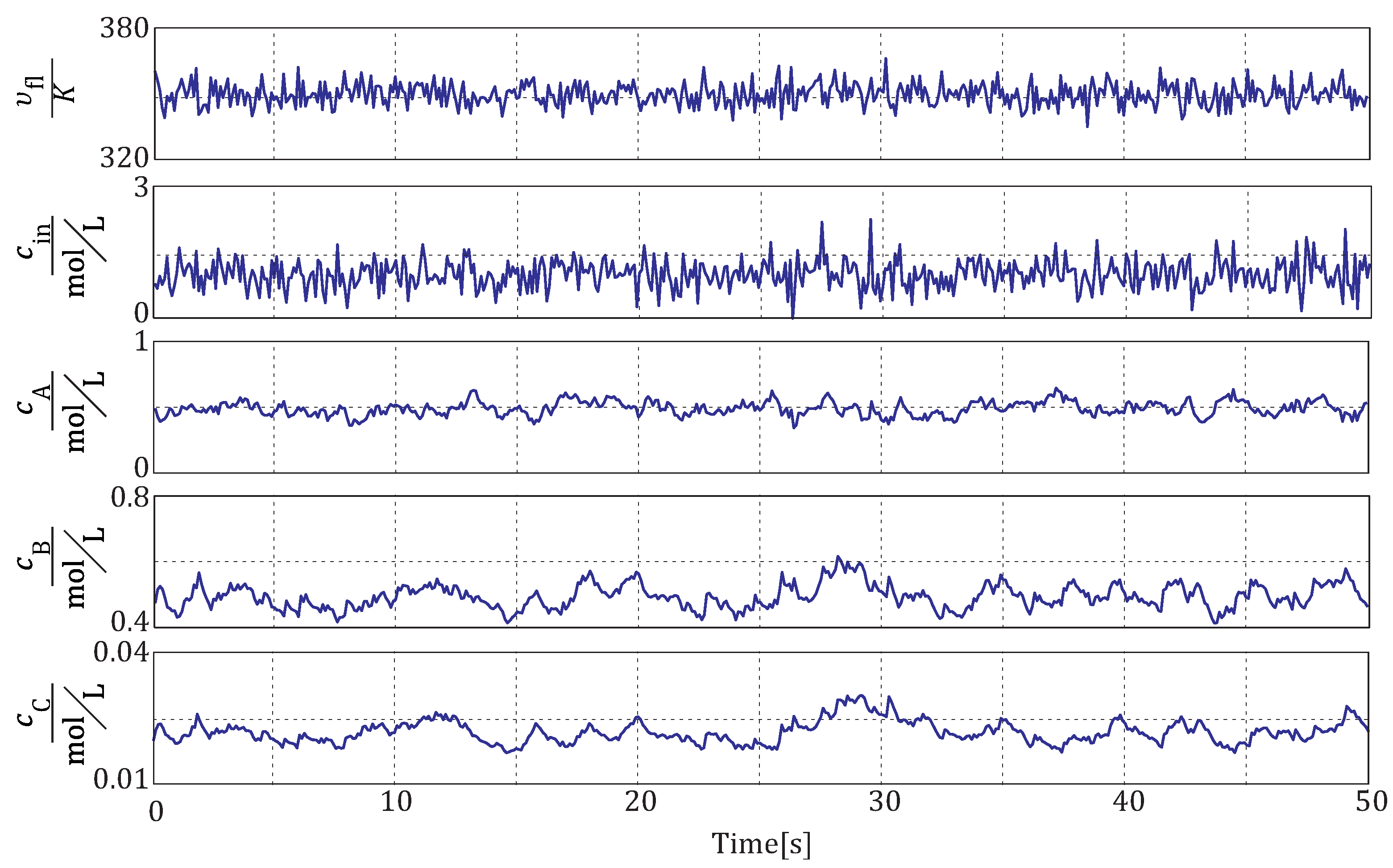
samples are used. An extract of the data set used for the analysis is given in
Figure 1. From the differential equations, it is expected that the methods deliver as a result the disturbance propagation path
.
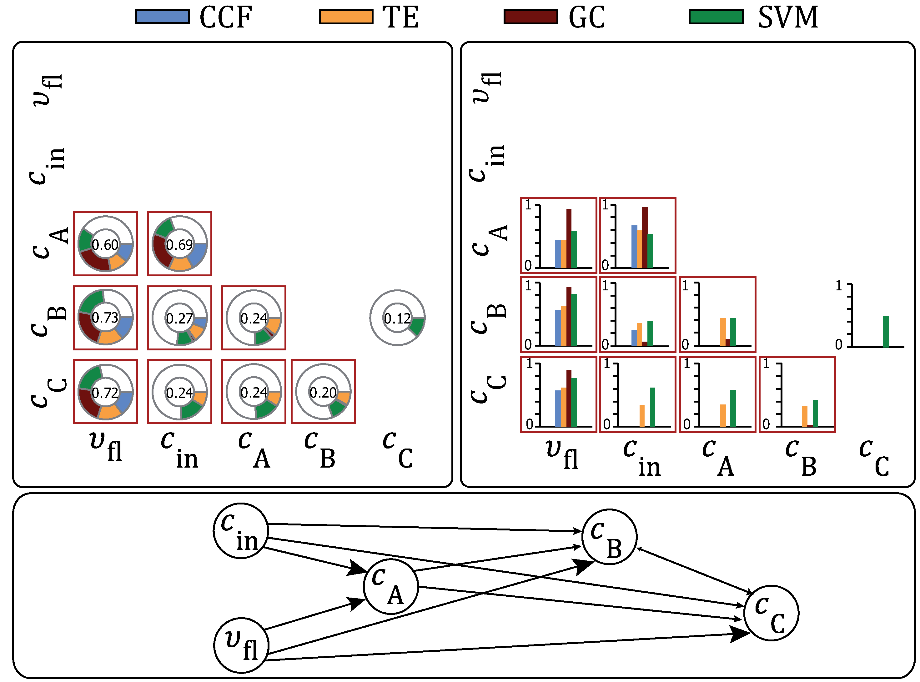
should be ranked in first position, since it has an impact on all three chemical reactions.
The results are illustrated in
Figure 2, with the red squares marking the expected causal dependencies. The design parameters result in
,
and
.
Figure 1.
Simulated data from the CSTR used for the analysis.
Figure 1.
Simulated data from the CSTR used for the analysis.
Figure 2.
Causal matrices for the stirred-tank-reactor. The red squares describe the expected causal dependencies to be detected by the methods.
Figure 2.
Causal matrices for the stirred-tank-reactor. The red squares describe the expected causal dependencies to be detected by the methods.
Analyzing the bar chart in
Figure 2 illustrates that all methods detect a large causal strength of
pointing towards the other process variables. This becomes obvious when taking into account the underlying differential equations of the CSTR (see Equation (
23)), as the temperature has a direct impact on all three concentrations. Furthermore, the result indicates that the nonlinearity implied in the exponential function has been correctly fitted by the Granger causality and cross-correlation function. Another strong causal strength has been found from
. This can also be explained through the differential equations, as
has a direct impact on
. The relationship
is the only indirect causal dependency detected by all methods, and
and
are detected by GC, TE and the SVM. The cause-effect dependency
and
has been found by TE and the SVM. Except the SVM, which detects the wrong causal dependency
, no wrong causal dependencies are found by the other methods. Furthermore, the transfer entropy is the only method that detects all expected causal dependencies. The propagation path from the combination of the methods is given in
Table 3.
Table 3.
Root cause priority list calculated from the causal matrix in
Figure 2.
Table 3.
Root cause priority list calculated from the causal matrix in Figure 2.
| Rank | Process variable | RC |
|---|
| 1 | | |
| 2 | | |
| 3 | | |
| 4 | | |
| 5 | | |
The resulting root cause priority list is given in
Table 3.
is correctly detected as being the root cause, and
, being the source of disturbances, is ranked second. Furthermore, the results show that causal dependencies at the end of the reaction chain result in weaker causal strengths or that these dependencies do not pass significance tests. The reason is that the disturbances are low-pass filtered each time a reaction takes place, so that less fluctuations for inferring causal dependencies are present in the data. Additionally, when merging the methods into one resulting causal matrix, the correct causal dependencies obtain a much stronger weighting compared to the causal matrices resulting from only one method at a time.
Figure 3.
Experimental setup of the laboratory plant.
Figure 3.
Experimental setup of the laboratory plant.
5.2. Experimental Laboratory Plant
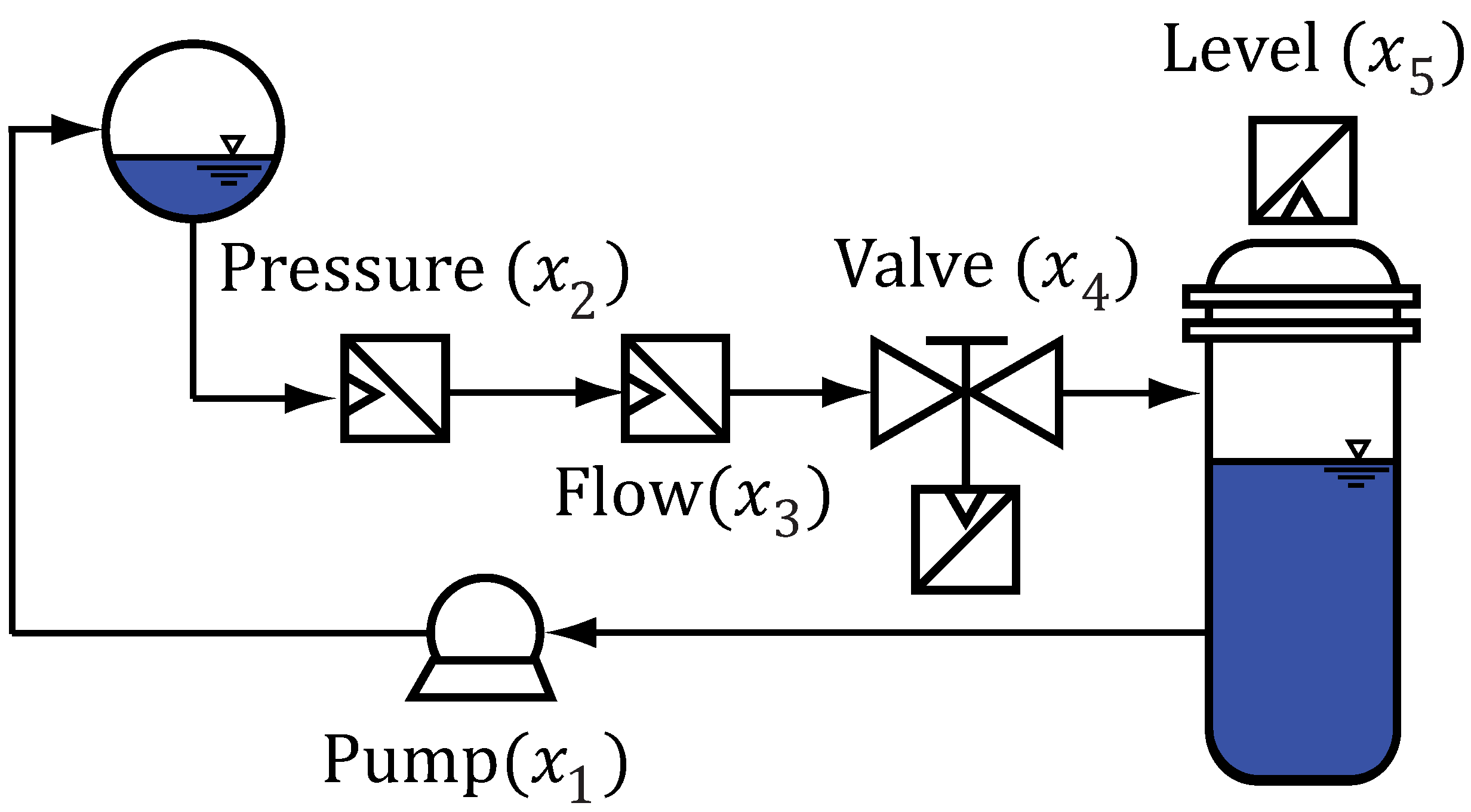
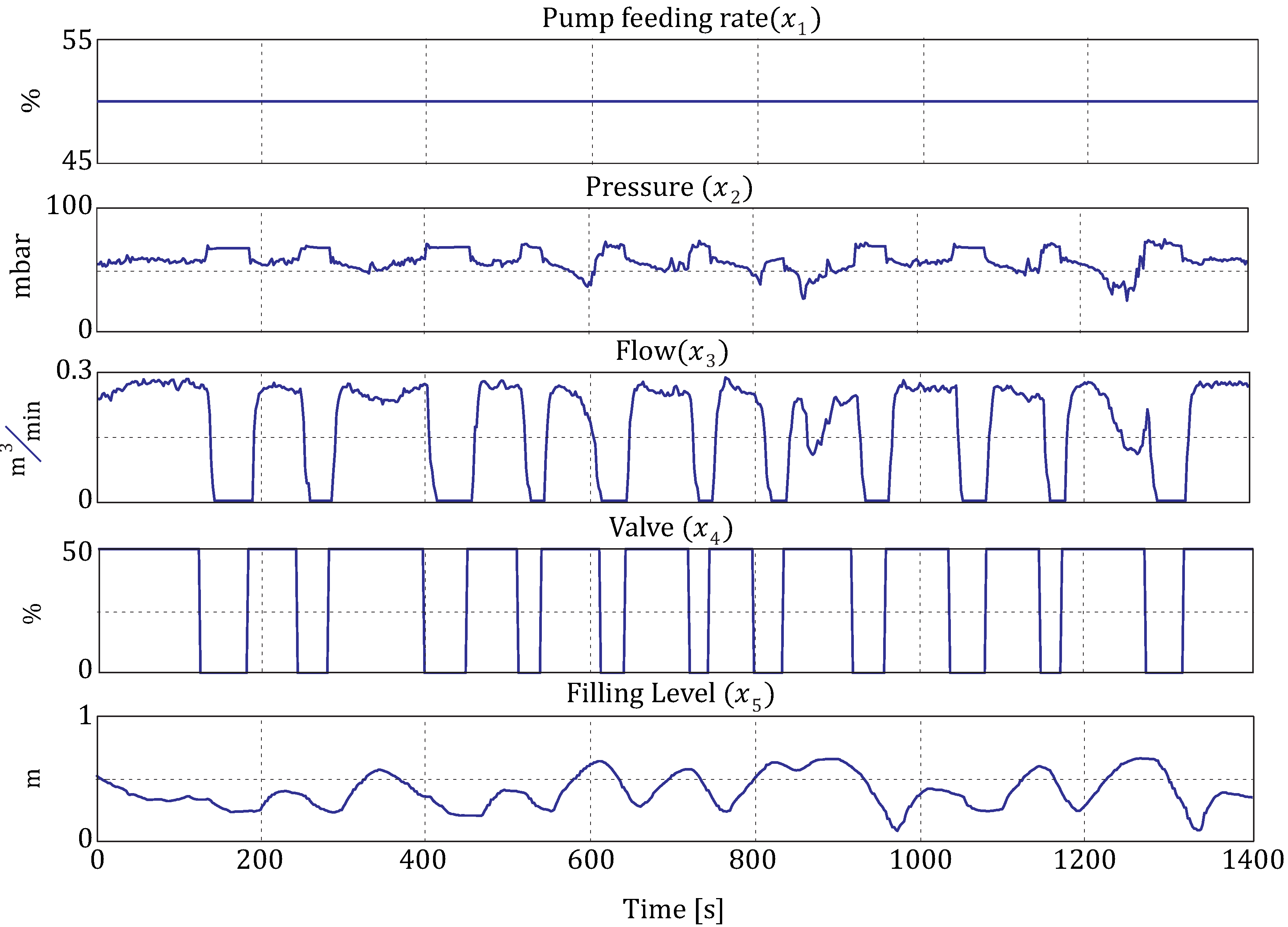
To evaluate the methods on real-world data, a fault is generated in an experimental laboratory plant that pumps water in cycles. A photo of the plant is given in
Figure 4, and the connection of the different process devices is sketched in
Figure 4. The process starts by setting a pump (
) positioned on the lower side of the plant into feed-forward control to transfer water into the ball-shaped upper tank. From the upper tank, the water passes several measurement devices before flowing into a lower cylindrical tank. Finally, the water flows from the lower tank back to the pump and closes the water cycle. Between the two tanks, pressure (
) and flow (
) are measured. With a valve (
), placed between the flow meter and the lower tank, the water flow can be controlled. Additionally, the filling level (
) is measured in the lower tank.
Figure 4.
Schematic drawing of the laboratory plant.
Figure 4.
Schematic drawing of the laboratory plant.
To generate a fault, a connection cable between the valve and compressor is removed and reattached randomly. The pump is set to 50% of its maximum feeding rate. The resulting data are illustrated in
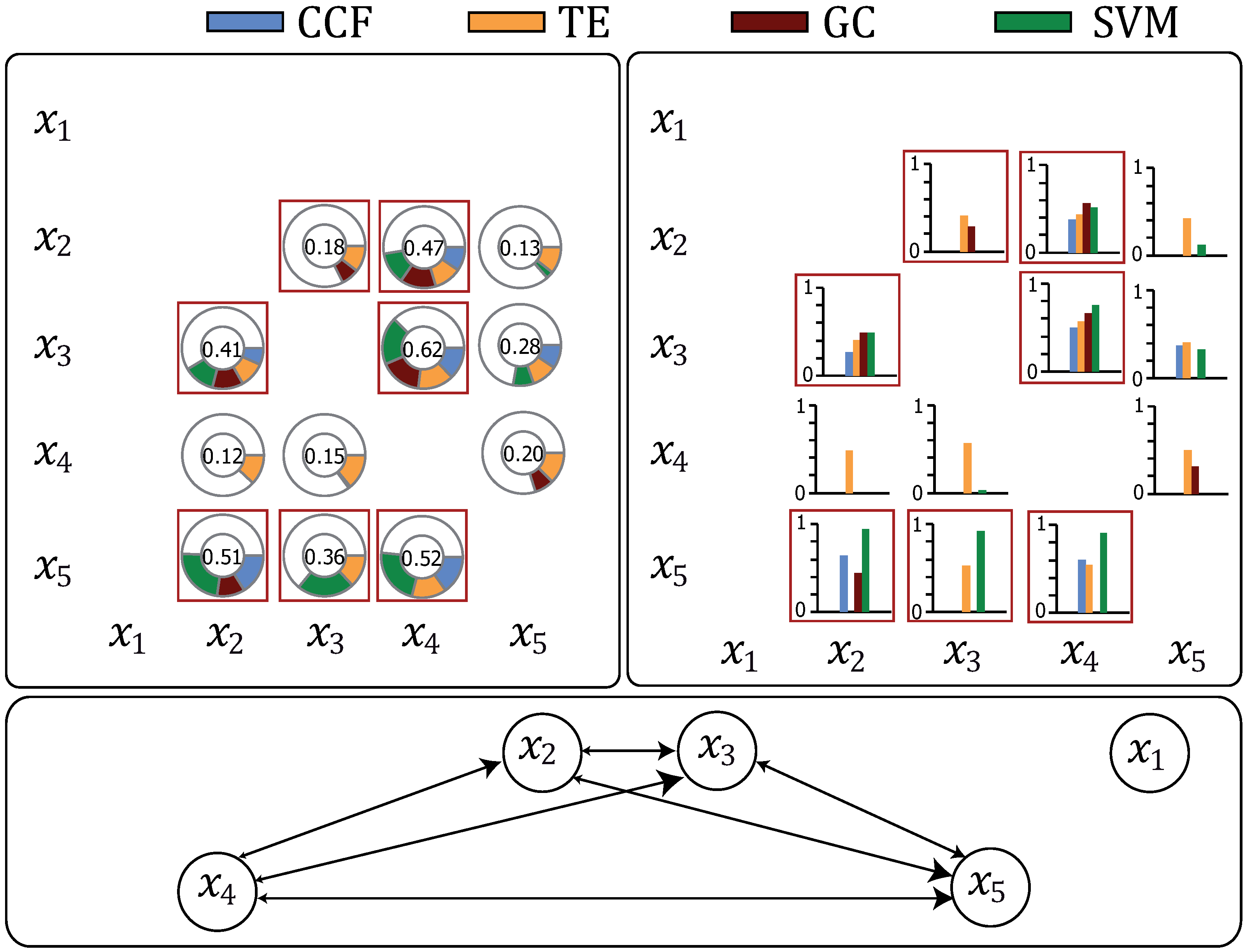
Figure 5. The instance the valve closes, the water is blocked from flowing from the upper to the lower tank. As it reopens, the process goes back into stationary phase. This means for the process variables that the flow reduces, while the level meter measures a continuous reduction of the water in the lower tank. The hydraulic pressure increases, until the pump stops delivering water from the lower to the upper tank. It is expected that the valve (
) is detected as being the root cause of the disturbance. The results are given in
Figure 6, where the red squares mark the expected causal dependencies, and the design parameters result in
,
and
.
No method can detect all expected causal dependencies, but all expected causal dependencies are found by at least two methods.
Table 4 gives the root cause priority list from the combined causal matrix. The valve is set on position one and is therefore correctly detected as being the root cause of the fault.
Like in the data from the CSTR, the outcome shows that when merging the methods into one resulting causal matrix, the correct causal dependencies obtain in a stronger weighting, meaning that the wrongly detected causal dependencies from some methods become less relevant.
Figure 5.
Data of the laboratory plant when having a faulty valve. Sampling rate .
Figure 5.
Data of the laboratory plant when having a faulty valve. Sampling rate .
Figure 6.
Causal matrices for the laboratory plant. The red squares describe the expected causal dependencies to be detected by the methods.
Figure 6.
Causal matrices for the laboratory plant. The red squares describe the expected causal dependencies to be detected by the methods.
Table 4.
Root cause priority list calculated from the causal matrix in
Figure 6.
Table 4.
Root cause priority list calculated from the causal matrix in Figure 6.
| Rank | Process Variable | RC |
|---|
| 1 | Valve opening () | 1.61 |
| 2 | Pressure () | 1.04 |
| 3 | Flow () | 0.69 |
| 4 | Filling level () | 0.61 |
| 5 | Pump feeding rate () | 0 |
6. Conclusion and Future Work
Several data-driven methods have been proposed to detect causal dependencies in measurements by exploiting information contained in time-shifts and statistical relationships.
As use cases, the methods were applied to backtrack the disturbance propagation path and localize the root cause with data coming from a simulated stirred-tank reactor and from a laboratory plant. In both cases, the causing variable of the fault was found correctly. Additionally, the results of the use cases showed, that it seems to be useful that more than one method is applied to perform an analysis. Since a found causal dependency is only a hypothesis, it gives more evidence if different methods indicate the same causal dependencies.
There is much room for future research. As all proposed methods localize faults solely from process data, one part of future work will focus on the integration of prior knowledge available from a plant (e.g., through the scheme of the plant or known process characteristics). Additionally, attenuation of fluctuations along their propagation through the system can be used as a further source of information for reconstructing the propagation path. Another topic is how the methods can be extended to work on MIMO systems, as it is also possible that two faults occur at the same time in a plant. Finally, the approach for combining the methods shows good results, but is rather ad hoc. Approaches using fuzzy decision making or Bayesian statistics need to be investigated.


