Automated Mounting of Pole-Shoe Wedges in Linear Wave Power Generators—Using Industrial Robotics and Proximity Sensors

Abstract

A system for automatic mounting of high tolerance wedges inside a wave power linear generator is proposed. As for any renewable energy concept utilising numerous smaller generation units, minimising the production cost per unit is vital for commercialization. The linear generator in question uses self-locking wedges, which are challenging to mount using industrial robots due to the high tolerances used, and because of the fact that any angular error remaining after calibration risks damaging the equipment. Using two types of probes, mechanical touch probes and inductive proximity sensors, combined with a flexible robot tool and iterative calibration routines, an automatic mounting system that overcomes the challenges of high tolerance wedge mounting is presented. The system is experimentally verified to work at mounting speeds of up to 50 $\mathrm{m}\mathrm{m}{\mathrm{s}}^{-1}$, and calibration accuracies of 0.25 $\mathrm{m}\mathrm{m}$ and 0.1 ${}^{\circ }$ are achieved. The use of a flexible robot tool, able to move freely in one Cartesian plane, was found to be essential for making the system work.

1. Introduction

Renewable electrical energy generation is often performed using a number of smaller distributed generation units if compared to classical electricity generation, utilising a few larger power plants [1]. Reducing the production cost for each unit hence becomes a crucial part in commercialising any renewable energy concept based on multiple smaller units. In order to achieve this goal, the use of automated production lines becomes necessary [2]. The work presented is part of the wave power project at Uppsala University, Sweden [3], a project focused on using sea-floor mounted linear generators coupled to buoys at the water surface, in order to extract energy from ocean waves. The developed linear generator contains two main components related to the internal electrical machine: the stator and the translator (see Figure 1). Automating the production of the stator is under development [4,5], but the translator has not yet been subjected to any automation attempts. This paper will initiate this work by looking into the feasibility of automating the mounting of the so-called pole-shoes, positioned on the translator’s central-pipe, using a concept based on self-locking wedges. Mounting these wedges is a challenging task due to the fine tolerances used, and the fact that any angular error present during the assembly process risks the wedge going into a state of premature self-locking, which can damage the pipe and equipment. In addition to differences between input components, there is also a secondary challenge in the sheer number of pole-shoes used in each translator, over 200, each with their own unique position.

There are numerous ways for a robot to obtain information about its surroundings, as mentioned in [6], all with their own advantages and disadvantages, and, in this application, a system is needed that is able to detect and account for individual differences between input components, also called workpieces. For the workpieces discussed here, the differences mainly come in the form of small angular deviations and differences in size, most often less than 0.1 ${}^{\circ }$ and 0.1 $\mathrm{m}\mathrm{m}$, respectively. Another source of errors is random differences in how the robot tool grips the workpiece relative to the robot’s coordinate system, and how they have been fed into the robot cell to begin with. To be able to compensate for these errors, a sensory system able to detect both the contour/edges and depth/distance of the presented objects is needed. This in order to be able to calculate both the translation and orientation of the workpiece. The idea of such a calibration system is not new and has been explored in the past by, for example, [7,8] , mostly relying on vision systems. Many modern vision systems also incorporate some kind of workpiece or object calibration capability, as this is a common task found in the industry.

This paper aims to answer two main questions related to the problems described above. Firstly, is it possible to obtain the calibration accuracy needed to mount high tolerance (±0.05 $\mathrm{m}\mathrm{m}$) wedges using a standard industrial robot without using high-cost sensors, vision and force-feedback systems, in order to keep project costs down during this initial evaluation stage? Secondly, what type of sensor would be the best to use in order to realise this task? Initial low-cost suggestions are inductive proximity sensors or touch probes, as they have been proven to work for similar applications in the past—for example, by [9], evaluating inductive proximity sensors for workpiece calibration, and, by [10], evaluation touch probes for robot calibration. Finally, to limit the scope of this first investigation, only the pole-shoe and central-pipe will be addressed. All other parts contained within the translator will subsequently be ignored.

2. Method

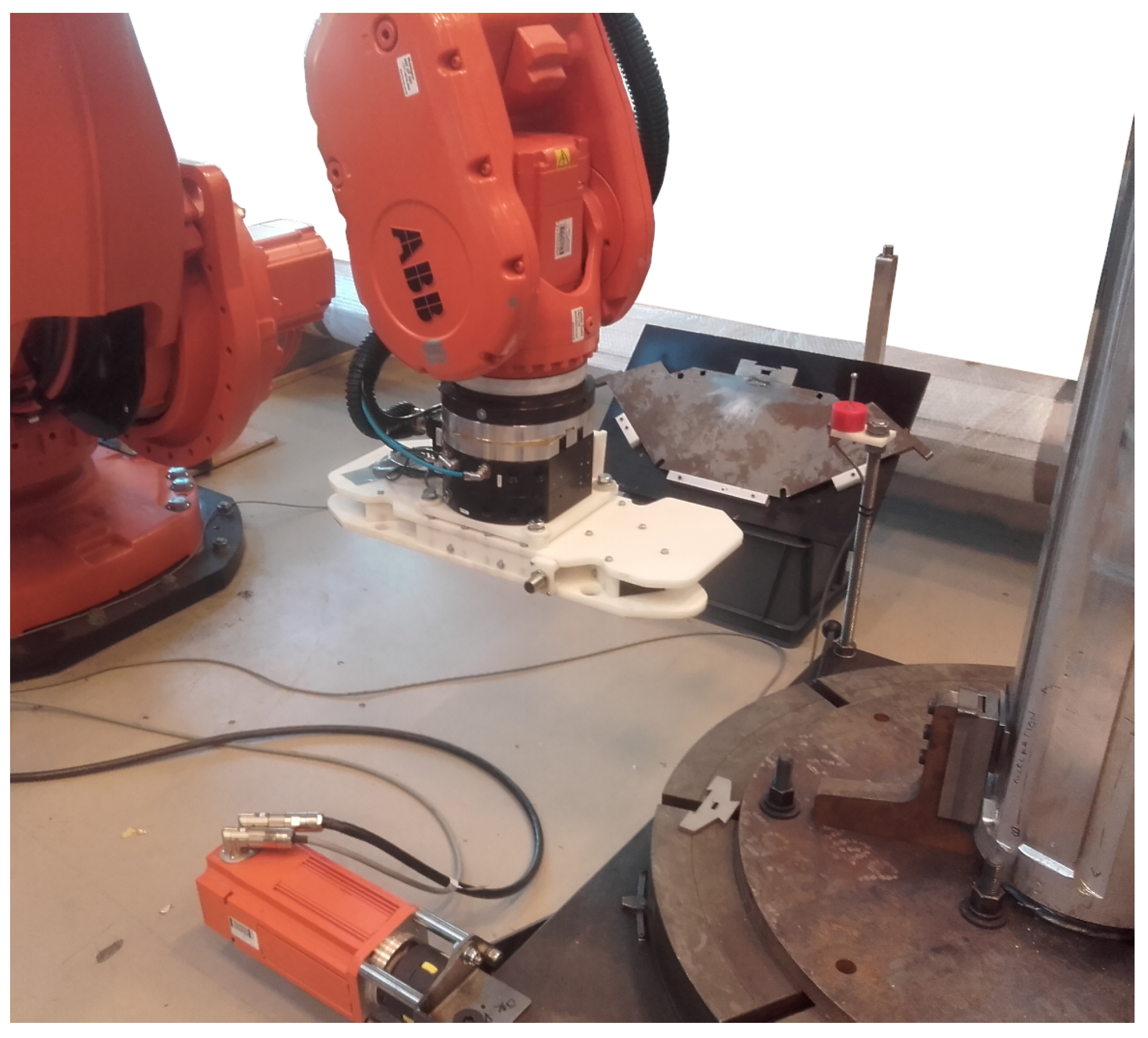
2.1. Experimental Setup

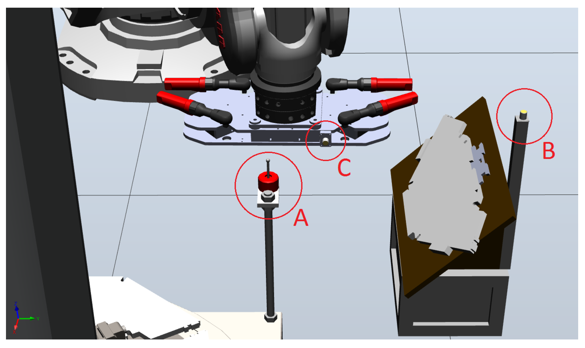
The robot used for these experiments was a floor mounted ABB6650S, shown in Figure 2. Next to the robot is a rotational table, carrying the central pipe of the translator. The secondary smaller table is used as storage for the pole-shoes. Mounted on the end of the robotic arm is a robot tool, designed to lift and manipulate the pole-shoes. Three main sensors were mounted in the cell, one touch probe and two inductive proximity sensors, shown in Figure 3. The touch probe (Sensor A) and one inductive proximity sensor (Sensor B) was mounted in proximity to the pole-shoe storage and were used to measure the orientation and translation of the pole-shoes, once lifted by the robot tool. The second inductive proximity sensor (Sensor C) was mounted on the robot tool itself and was used to measure the orientation and position of the central pipe. This setup creates a system with 7-DOF (Degrees of Freedom), 6-DOF for the robot and 1-DOF for the pipe, which need to be simultaneously controlled or otherwise accounted for. The accuracy of the robot for repeated motions was specified to ±0.1 $\mathrm{m}\mathrm{m}$ and ±0.1 ${}^{\circ }$. This puts an upper limit on the accuracy needed in the measurement system, as any measurement more accurate than this would be wasted in regards to robot positioning.

The robot’s movements and actions were controlled using programs written in the RAPID programming language. Detailed definitions of all RAPID-related terms and commands can be found in the RAPID manual [11]. RAPID-related terms will be marked with the TELETYPE font for easy recognition. In order to realise the pole-shoe mounting and calibration, a set of additional functions were developed, in addition to the standard RAPID language. Their implementation can be found in the supplementary file EXTRA_ RAPID_ FUNCTIONS_ V1.TXT.

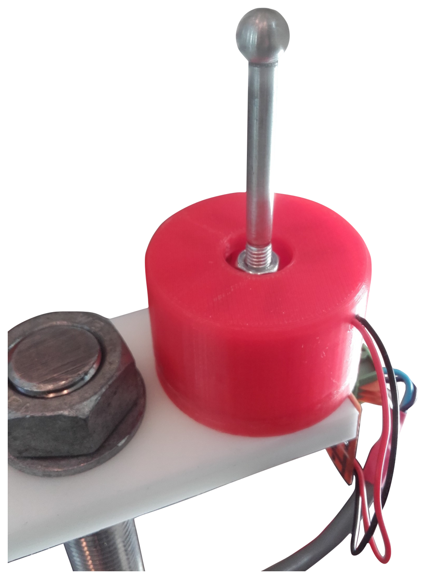
2.1.1. The Touch Probe

The purpose of a touch probe is to be able to detect contact with any solid object from any direction, relative to the sensor’s tip, except the direction occupied by the probe itself. Numerous commercial touch-probes are available, with accuracies down to less than a few μm, and prices starting at around 500 USD. This level of accuracy was, however, not necessary in this application, as the robot itself had a specified accuracy of ±0.1 $\mathrm{m}\mathrm{m}$. Therefore, a custom probe, shown in Figure 4, was constructed using cheap, easily available electrical components and a 3D-printed plastic chassis. The design of the developed touch-probe is based on the designs presented in the patents US 4547971-A, US 4769919-A and US 4153998-A. The total material cost for the touch probe was approximately 10 USD. This cost is in the same range as the used inductive proximity sensors (OMRON-E2A), costing around 40 USD each.

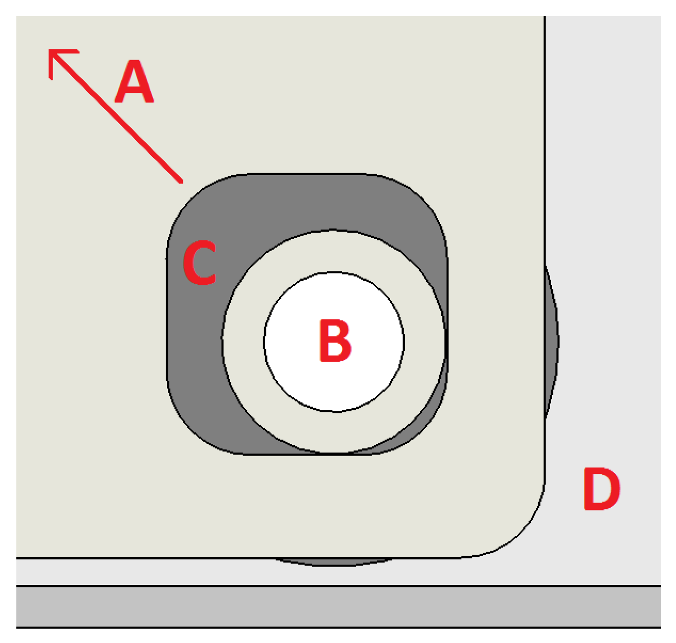
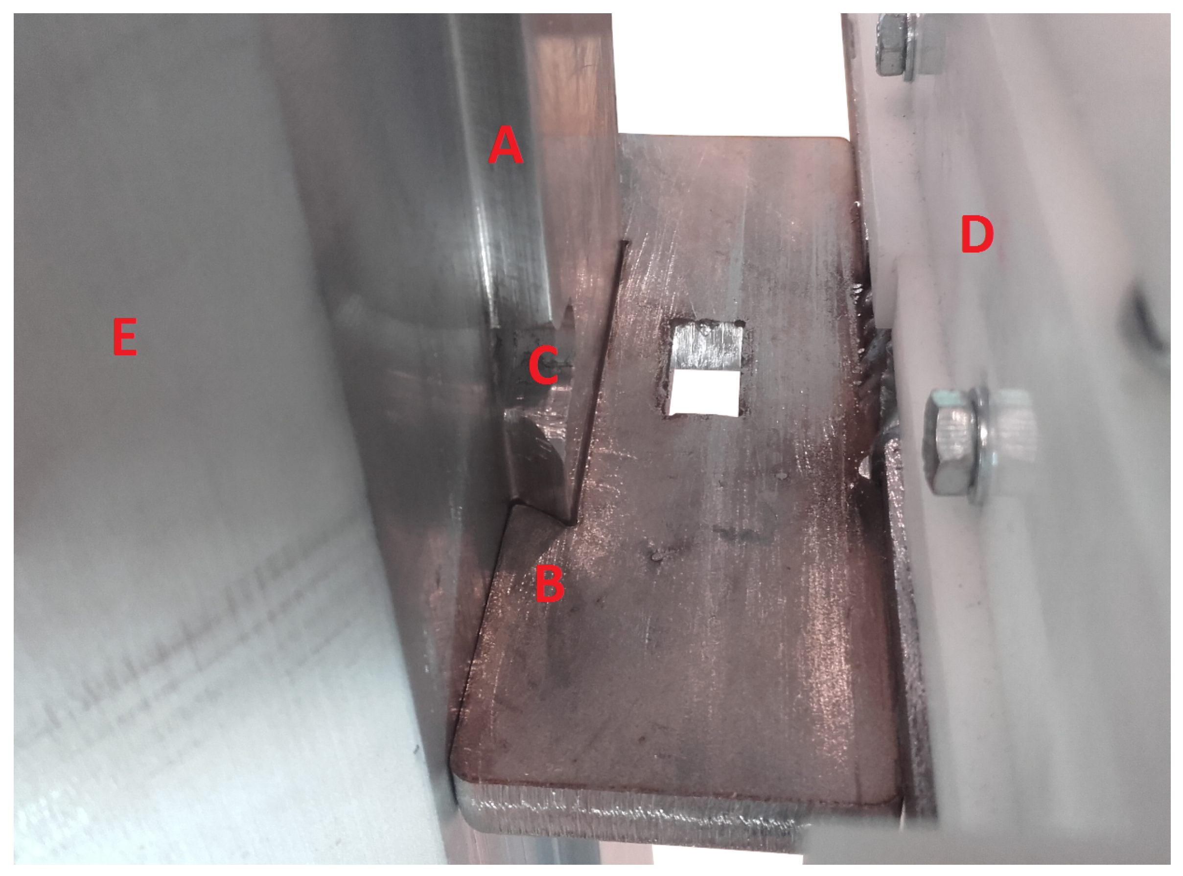
2.1.2. The Electromagnet Tool

The tool used to lift the pole-shoes was based on current-controlled electromagnets, described more closely in [12]. The tool was also equipped with a planar sliding mechanism that allowed an external force to displace the tool up to ±2 $\mathrm{m}\mathrm{m}$ in the Cartesian $xy$-plane while remaining locked in the z-direction. This was achieved by mounting the locking bolts of the tool in square holes with a side length longer than the diameter of the fastening bolt, as shown in Figure 5. To make sure that the tool always returned to the same position, a set of pre-tensioned springs was used.

2.2. Calculating a Quaternion from Three Points

In order to use sensory data to correct for tool and work-object errors, understanding the robots positioning system is crucial. There are numerous ways to represent an orientation, or rotation, and position in 3D space. The way chosen in this paper was to use Cartesian-coordinates for positions and quaternions for rotations, as this is the representation used within RAPID. However, since the used sensors were only able to measure single points in space, a method of converting between points and quaternions was needed.

To do this, let the 3D-vectors ${\mathbf{v}}_{\mathbf{x}}=[x_1,y_1,z_1]$, ${\mathbf{v}}_{\mathbf{y}}=[x_2,y_2,z_2]$, ${\mathbf{v}}_{\mathbf{z}}=[x_3,y_3,z_3]$ and the point $p_s=[x_s,y_s,z_s]$ be defined by a set of three unique input points ($p_0$, $p_1$, $p_2$ or $p_5$, $p_6$, $p_7$) and one of the following set of equations

$$\begin{array}{cc}\hfill p_s& =p_0+(p_1-p_0)s,s\in [0,1],\hfill \end{array}$$

(1a)

$$\begin{array}{cc}\hfill {\mathbf{v}}_{\mathbf{x}}& =\frac{p_2-p_s}{\left|\right|p_2-p_s\left|\right|},\hfill \end{array}$$

(1b)

$$\begin{array}{cc}\hfill {\mathbf{v}}_{\mathbf{y}}& =\frac{p_s-p_1}{\left|\right|p_s-p_1\left|\right|},\hfill \end{array}$$

(1c)

$$\begin{array}{cc}\hfill {\mathbf{v}}_{\mathbf{z}}& ={\mathbf{v}}_{\mathbf{x}}\times {\mathbf{v}}_{\mathbf{y}},\hfill \end{array}$$

(1d)

$$\begin{array}{cc}\hfill 0& ={\mathbf{v}}_{\mathbf{x}}•{\mathbf{v}}_{\mathbf{y}},\hfill \end{array}$$

(1e)

or

$$\begin{array}{cc}\hfill p_s& =p_5+(p_6-p_5)s,s\in [0,1],\hfill \end{array}$$

(2a)

$$\begin{array}{cc}\hfill {\mathbf{v}}_{\mathbf{x}}& ={\mathbf{v}}_{\mathbf{y}}\times {\mathbf{v}}_{\mathbf{z}},\hfill \end{array}$$

(2b)

$$\begin{array}{cc}\hfill {\mathbf{v}}_{\mathbf{y}}& =\frac{p_7-p_s}{\left|\right|p_7-p_s\left|\right|},\hfill \end{array}$$

(2c)

$$\begin{array}{cc}\hfill {\mathbf{v}}_{\mathbf{z}}& =\frac{p_6-p_s}{\left|\right|p_6-p_s\left|\right|},\hfill \end{array}$$

(2d)

$$\begin{array}{cc}\hfill 0& ={\mathbf{v}}_{\mathbf{y}}•{\mathbf{v}}_{\mathbf{z}},\hfill \end{array}$$

(2e)

where $p_0$, $p_1$, $p_2$ or $p_5$, $p_6$, $p_7$ define a plane in 3D-space. Note that the exact indices and the input order of the plane-defining points are different between Equations (1) and (2). Having two separate definitions was a way to handle the problem that the relative orientation between the measured points was different between the pole-shoe and pipe, as will be shown later.

Solving Equations (1) or (2) for the unknown scalar value, s, and substituting the answer back into the equations will generate a solution in which ${\mathbf{v}}_{\mathbf{x}}$, ${\mathbf{v}}_{\mathbf{y}}$ and ${\mathbf{v}}_{\mathbf{z}}$ are three orthogonal unit vectors and can therefore be used as the principal axes of a coordinate system. A normalised rotational matrix, $\mathbf{R}$, containing the vectors ${\mathbf{v}}_{\mathbf{x}}$, ${\mathbf{v}}_{\mathbf{y}}$ and ${\mathbf{v}}_{\mathbf{z}}$ can then be defined as

$$\mathbf{R}=\left[\begin{array}{ccc}{\mathbf{v}}_{\mathbf{x}.\mathbf{x}}& {\mathbf{v}}_{\mathbf{y}.\mathbf{x}}& {\mathbf{v}}_{\mathbf{z}.\mathbf{x}}\\ {\mathbf{v}}_{\mathbf{x}.\mathbf{y}}& {\mathbf{v}}_{\mathbf{y}.\mathbf{y}}& {\mathbf{v}}_{\mathbf{z}.\mathbf{y}}\\ {\mathbf{v}}_{\mathbf{x}.\mathbf{z}}& {\mathbf{v}}_{\mathbf{y}.\mathbf{z}}& {\mathbf{v}}_{\mathbf{z}.\mathbf{z}}\end{array}\right],$$

(3)

where ${\mathbf{v}}_{\mathbf{a}.\mathbf{b}}$ denotes element b of vector a.

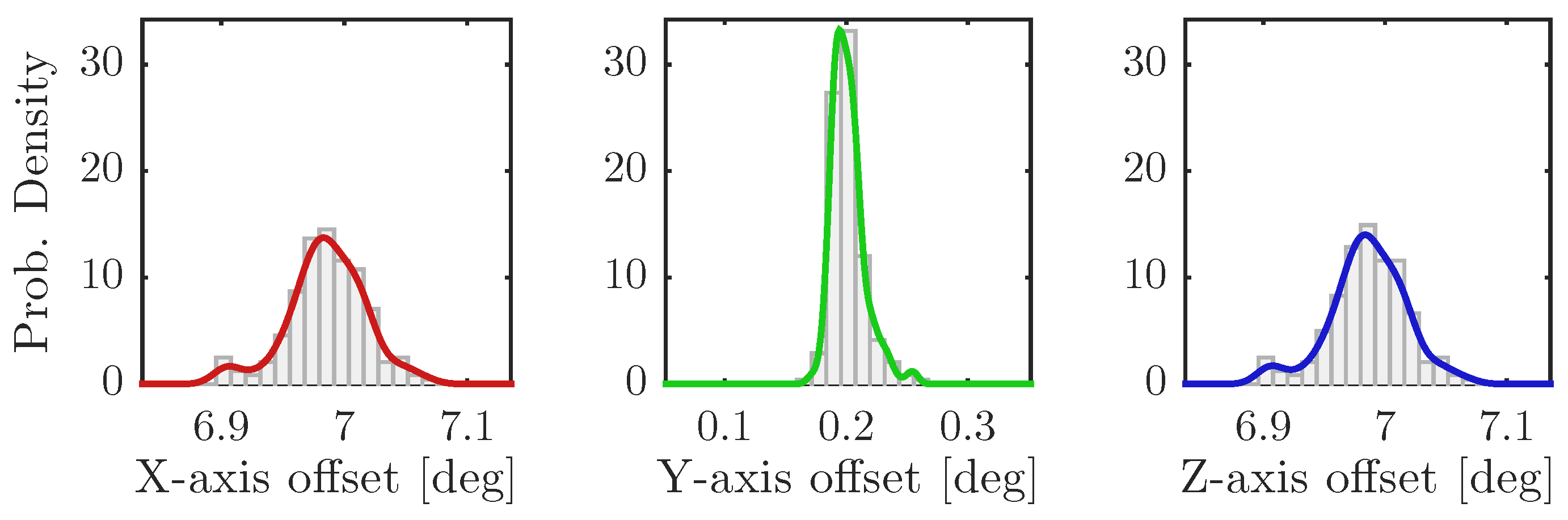
Also useful is the magnitude of the angular error, measured against each of the the principal axes, calculated by

$$\begin{array}{cc}\hfill {\alpha }_x& =arctan\left(\frac{\left|\right|[1,0,0]\times {\mathbf{v}}_{\mathbf{x}}\left|\right|}{[1,0,0]•{\mathbf{v}}_{\mathbf{x}}}\right),\hfill \end{array}$$

(4a)

$$\begin{array}{cc}\hfill {\alpha }_y& =arctan\left(\frac{\left|\right|[0,1,0]\times {\mathbf{v}}_{\mathbf{y}}\left|\right|}{[0,1,0]•{\mathbf{v}}_{\mathbf{y}}}\right),\hfill \end{array}$$

(4b)

$$\begin{array}{cc}\hfill {\alpha }_z& =arctan\left(\frac{\left|\right|[0,0,1]\times {\mathbf{v}}_{\mathbf{z}}\left|\right|}{[0,0,1]•{\mathbf{v}}_{\mathbf{z}}}\right),\hfill \end{array}$$

(4c)

where ${\alpha }_x$, ${\alpha }_y$ and ${\alpha }_z$ denotes the angular error measured against the Cartesian X, Y and Z principal axis, respectively.

While the above angular offsets present an intuitive way to represent the error, it is unfortunately not the representation used by the ABB6650s; instead, the robot control system uses quaternions. The conversion between a rotational matrix and a quaternion can be done using the following equations:

$$\begin{array}{cc}\hfill \mathbf{Q}& =[q_1,\mathbf{i}{q}_2,\mathbf{j}{q}_3,\mathbf{k}{q}_4],\hfill \end{array}$$

(5a)

$$\begin{array}{cc}\hfill {\mathbf{Q}}^{\ast }& =[q_1,-\mathbf{i}{q}_2,-\mathbf{j}{q}_3,-\mathbf{k}{q}_4],\hfill \end{array}$$

(5b)

$$\begin{array}{cc}\hfill q_1& =\mathbf{Re}\left(\frac{1}{2}\sqrt{{\mathbf{v}}_{\mathbf{x}.\mathbf{x}}+{\mathbf{v}}_{\mathbf{y}.\mathbf{y}}+{\mathbf{v}}_{\mathbf{z}.\mathbf{z}}+1}\right),\hfill \end{array}$$

(5c)

$$\begin{array}{cc}\hfill q_2& =\mathbf{Re}\left(\frac{2[{\mathbf{v}}_{\mathbf{y}.\mathbf{z}}⩾{\mathbf{v}}_{\mathbf{z}.\mathbf{y}}]-1}{2}\sqrt{{\mathbf{v}}_{\mathbf{x}.\mathbf{x}}-{\mathbf{v}}_{\mathbf{y}.\mathbf{y}}-{\mathbf{v}}_{\mathbf{z}.\mathbf{z}}+1}\right),\hfill \end{array}$$

(5d)

$$\begin{array}{cc}\hfill q_3& =\mathbf{Re}\left(\frac{2[{\mathbf{v}}_{\mathbf{z}.\mathbf{x}}⩾{\mathbf{v}}_{\mathbf{x}.\mathbf{z}}]-1}{2}\sqrt{{\mathbf{v}}_{\mathbf{y}.\mathbf{y}}-{\mathbf{v}}_{\mathbf{x}.\mathbf{x}}-{\mathbf{v}}_{\mathbf{z}.\mathbf{z}}+1}\right),\hfill \end{array}$$

(5e)

$$\begin{array}{cc}\hfill q_4& =\mathbf{Re}\left(\frac{2[{\mathbf{v}}_{\mathbf{x}.\mathbf{y}}⩾{\mathbf{v}}_{\mathbf{y}.\mathbf{x}}]-1}{2}\sqrt{{\mathbf{v}}_{\mathbf{z}.\mathbf{z}}-{\mathbf{v}}_{\mathbf{x}.\mathbf{x}}-{\mathbf{v}}_{\mathbf{y}.\mathbf{y}}+1}\right),\hfill \end{array}$$

(5f)

where $[{\mathbf{v}}_{\mathbf{a}.\mathbf{b}}⩾{\mathbf{v}}_{\mathbf{b}.\mathbf{a}}]$ is used as a logical operator, having a value of either 1 or 0. $\mathbf{Q}$ represents the complex four-dimensional quaternion and ${\mathbf{Q}}^{\ast }$ its complex conjugate. Note that during the implementation of these equations into the robot, the $\mathbf{Re}$ (real part) operator was replaced with an IF statement that checked if the sum under the square root was negative or not; if negative, the sum was set to zero. This was required since the sqrt(x) function in the RAPID language is unable to handle negative numbers. The result of the calculation remains the same, just less elegant. For the full RAPID implementation, please refer to Rotm2Quat in the supplementary file.

2.3. Pole-Shoe Calibration

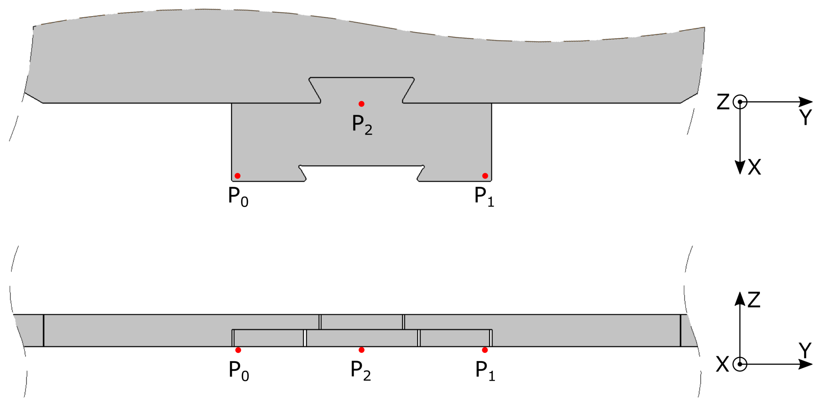
The tool position and orientation of the pole-shoe lifting tool is a 6-DOF problem that needs to be solved in order to calibrate the pole-shoe. This was done by having the robot find the coordinates of three points on the pole-shoe, here called $p_0$, $p_1$ and $p_2$ (defined relative to the BASE coordinate system of the robot, see Figure 6). Determining the coordinates of these points was done by using the digital output signal from either sensor A or B and the SearchL (Linear Search) RAPID command.

Once obtained, a pole-shoe orientation quaternion, ${\mathbf{Q}}_{\mathbf{shoe}}$, can be constructed using Equations (1) and (5). The full RAPID implementation of the equations, needed to calculate the pole-shoe’s orientation from the three points, can be found in the supplementary RAPID file under ShoePoints2Quat.

The calculated quaternion can be used to calculate an orientation error, ${\mathbf{Q}}_{err}$. This was done by configuring the tool, relative to the BASE coordinate system, in such a way that the measured points (for a perfectly aligned pole-shoe) would result in an unit rotational matrix, ${\mathbf{R}}_{unit}$, and unit quaternion, $Q_{unit}$, defined as

$$\begin{array}{cc}\hfill {\mathbf{R}}_{unit}& =\left[\begin{array}{ccc}1& 0& 0\\ 0& 1& 0\\ 0& 0& 1\end{array}\right],\hfill \end{array}$$

(6a)

$$\begin{array}{cc}\hfill {\mathbf{Q}}_{unit}& =[1,0,0,0].\hfill \end{array}$$

(6b)

This approach reduces the calculation of the orientation error into simply becoming the conjugate of the tool quaternion

$${\mathbf{Q}}_{err}={\mathbf{Q}}_{shoe}^{\ast }.$$

(7)

A better estimation for the correct tool-orientation, ${\mathbf{Q}}_{corr}$, can then be obtained by applying the Hamilton product, $\mathbf{H}$, between the original tool orientation, ${\mathbf{Q}}_{org}$ (the orientation of the tool at the time $p_0$, $p_1$ and $p_2$ was measured), and the error quaternion, written as

$${\mathbf{Q}}_{corr}=\mathbf{H}\left({\mathbf{Q}}_{err},{\mathbf{Q}}_{org}\right).$$

(8)

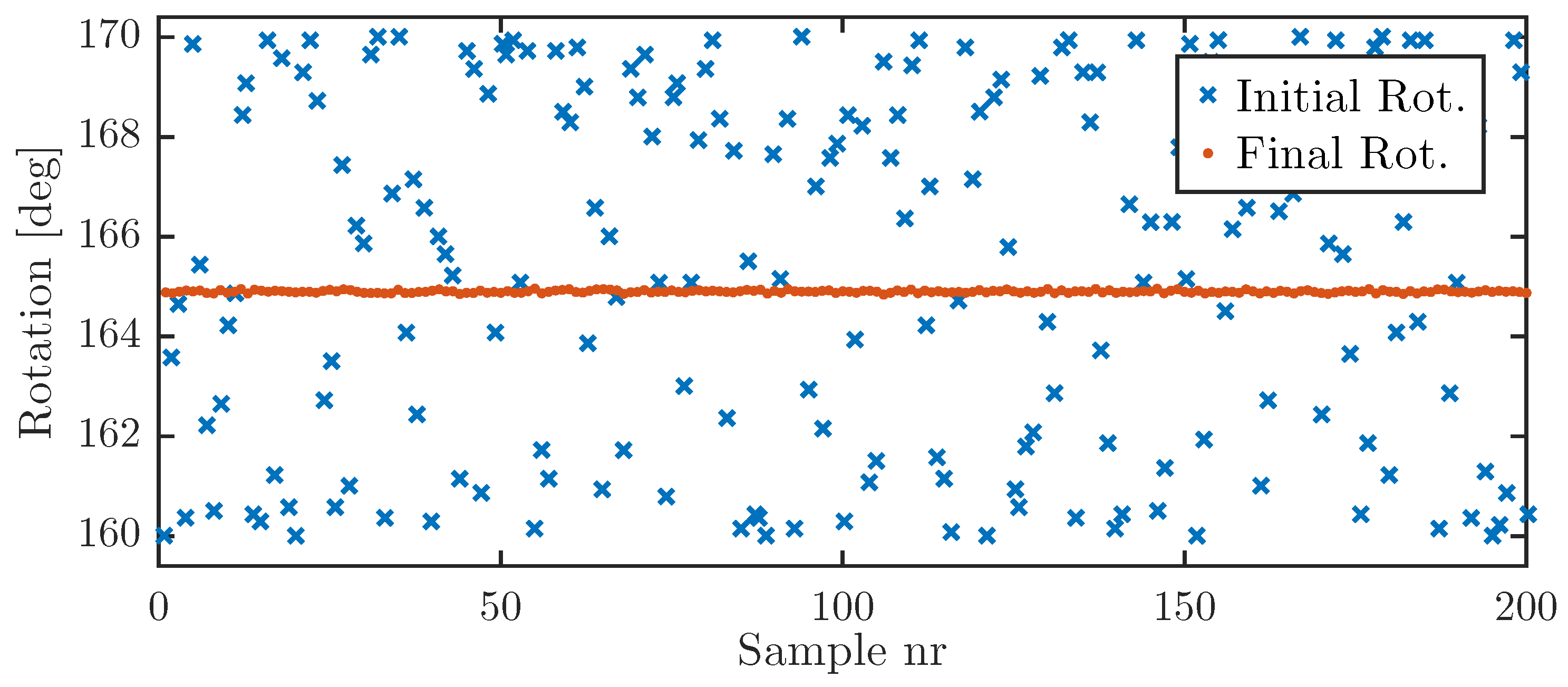
In the RAPID program, all of the above calculations were put into a loop where the robot would repeatedly measure and adjust for the resulting ${\mathbf{Q}}_{err}$. In addition, when the corresponding angular error reached below a set threshold, the calibration routine would abort and report a success; if not, it would repeat with the previous orientation estimate as the new initial tool orientation. For the RAPID implementation of the Hamilton product, please refer to HamProd in the supplementary file.

Once a good orientation of the pole-shoe tool had been obtained, it was copied into a tooldata-definition, a data-type used to define custom tools. This was done by using the fact that robot mounted tools, in RAPID, are defined relative to tool0, defined as the centre of the end plate on the final joint of the robot. Obtaining the relative orientation between tool0 and the current active tool, here called ${\mathbf{Q}}_{tool}$, can be done by using the CRobT-command, with tool0 and wobj0 as references. In addition to describing the rotation of a tool, the tooldata data type contains information about the translation of the tool centre point (TCP) and also stores the tool’s kinematic properties. During these experiments, only the translation and orientation were updated after each measurement. The kinematic properties were assumed to be constant.

The tool’s TCP was defined as $p_1$ in Figure 6, and its position relative to tool0 was calculated by taking the difference between the known position of the used sensor (A or B), and the recorded position of tool0 when the sensor was triggered at the position for $p_1$. To get the actual TCP offset, this difference then had to be rotated, using the Hamilton product, to account for the difference in orientation between the BASE and tool coordinate systems.

Using an orientation directly copied from tool0 as the base for correcting the active tool simplified further positioning-programming, since the robot would report a unit quaternion rotation if the active tool was perfectly aligned towards the currently active coordinate system and if the Hamilton correction was done correctly.

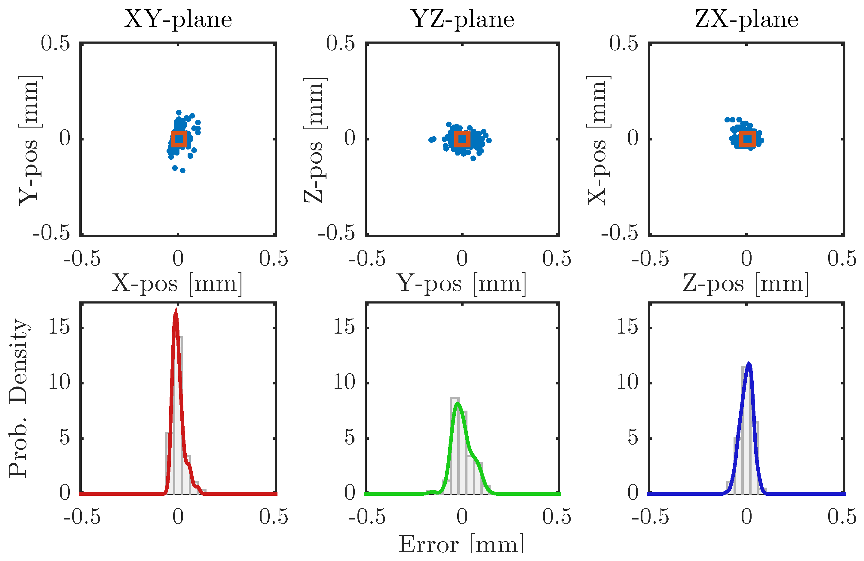
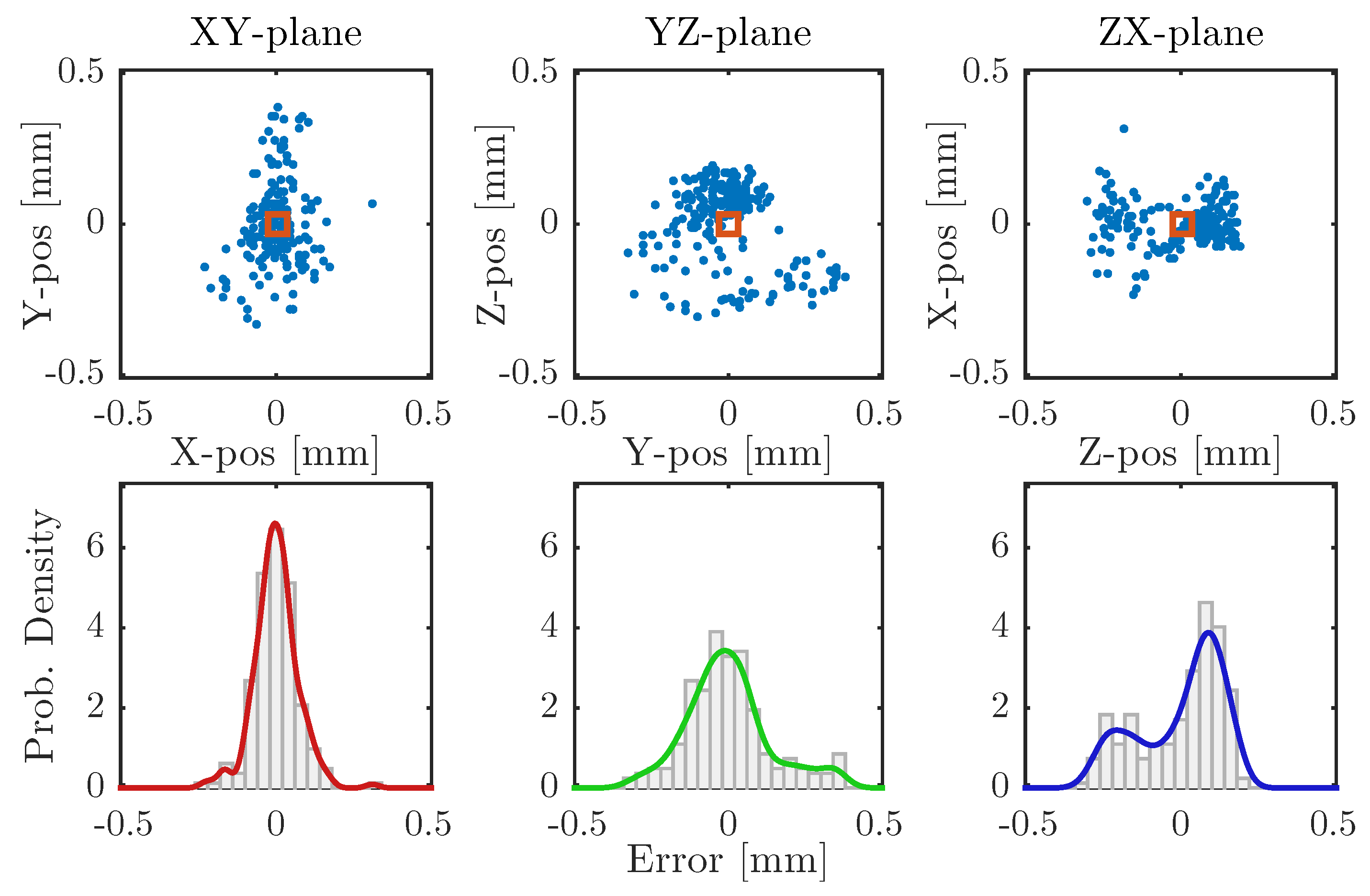
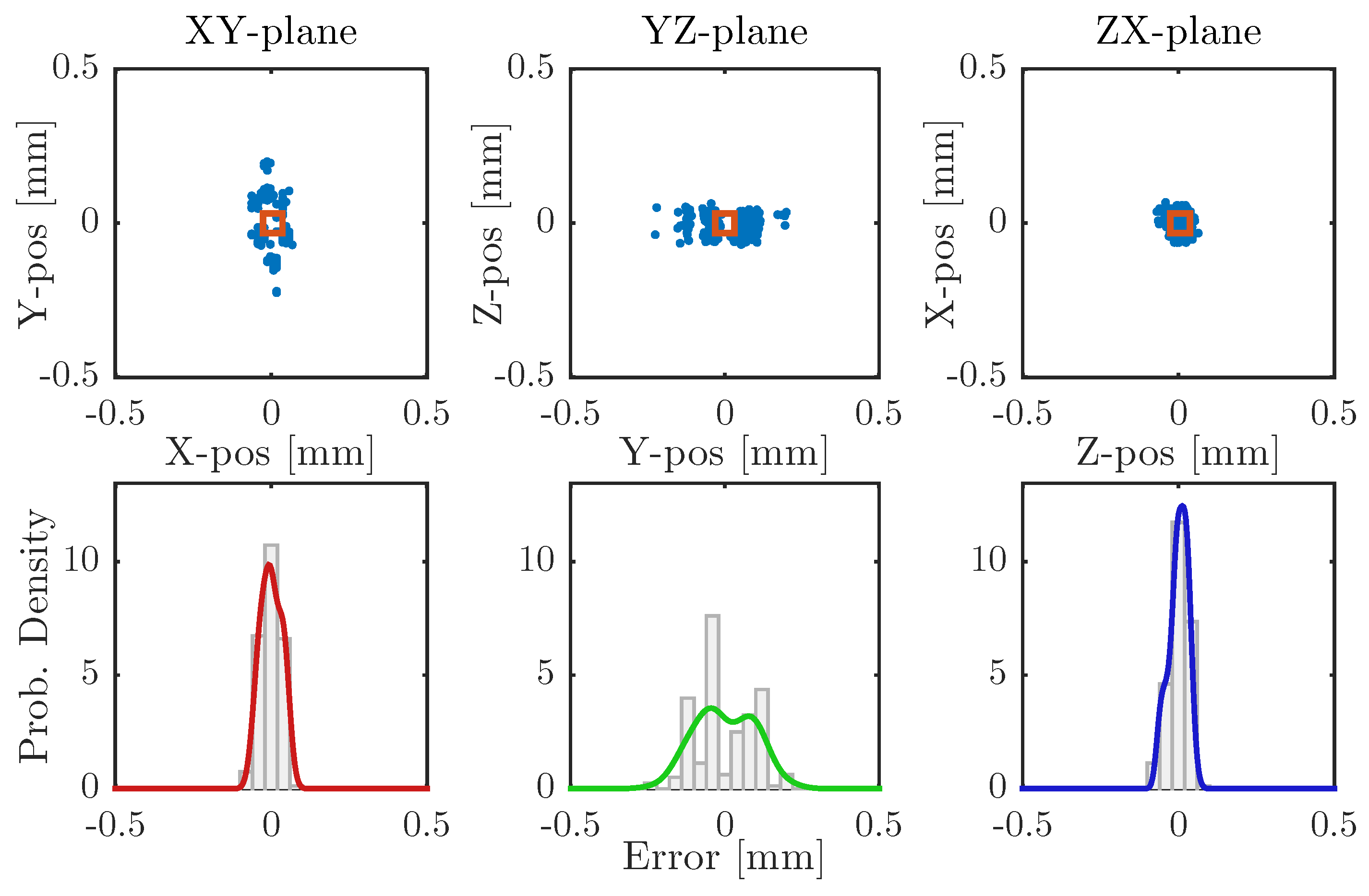
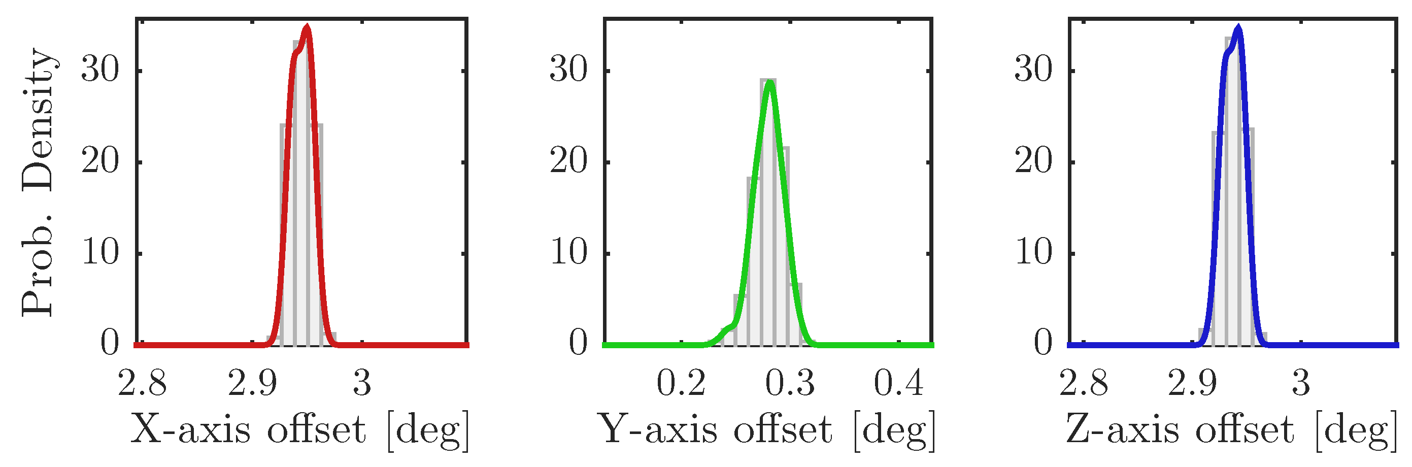
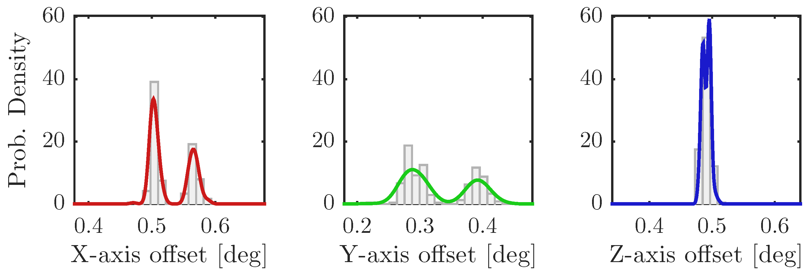
The pole-shoe calibration routine was evaluated using two different sensors: the inductive proximity sensor and the touch probe. In order to evaluate if there was any difference in performance between the two, where the main evaluation criteria were repeatability and absolute error.

2.4. Central-Pipe Calibration

The calibration procedure of the central pipe was implemented similarly to that of the pole-shoe. However, since the pipe could only move around the z-axis (relative to the BASE coordinate system), as it was mounted on a rotational table, the procedure was split into two separate steps. The first step oriented the main wedge surface of the central pipe to be roughly aligned with the BASE coordinate system. The second step then measured the remaining orientation and translation error of the pipe and calculated a corresponding work object coordinate system, so that the principal axes of the work-object were aligned to the pipe’s surfaces.

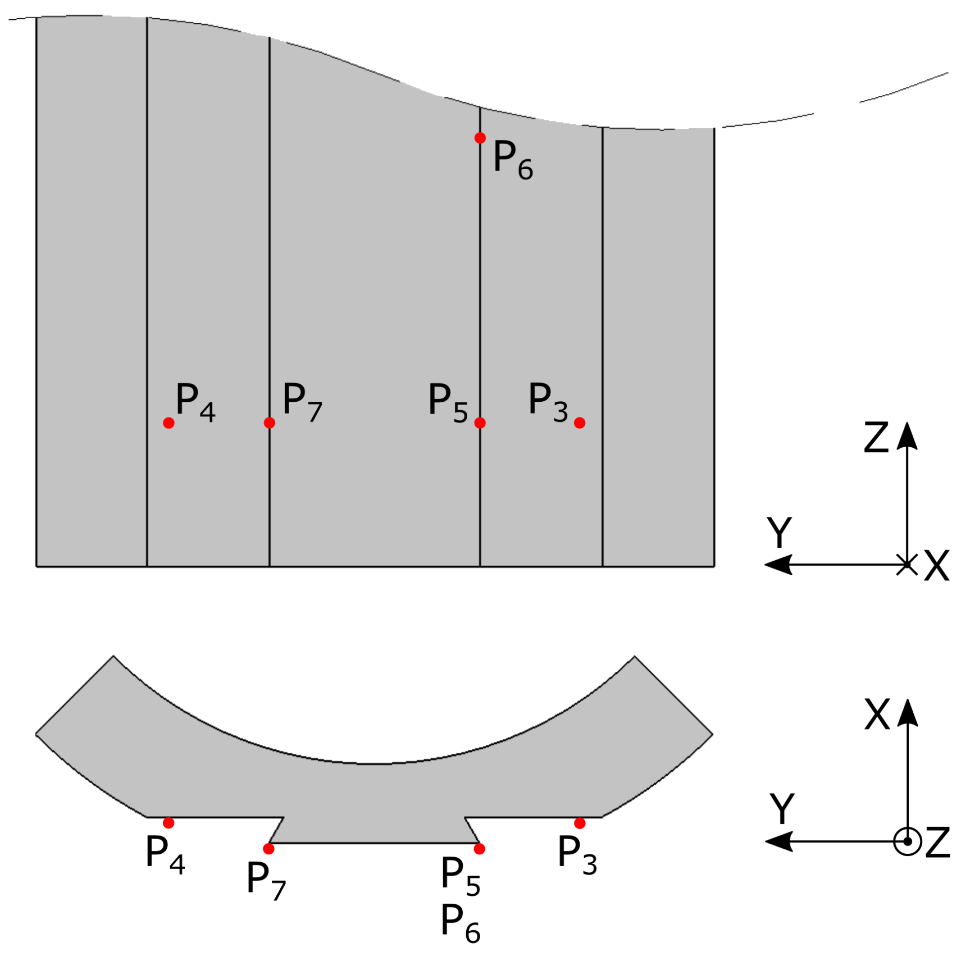
To align the main surface, two initial points ($p_3$ and $p_4$) were measured using the tool mounted inductive sensor (Sensor C) (see Figure 7). The angular orientation error, ${\alpha }_{err}$, around the pipe’s z-axis was then estimated by

$${\alpha }_{err}=arctan\left(\frac{p_{4.x}-p_{3.x}}{p_{4.y}-p_{3.y}}\right).$$

(9)

The pipe was automatically rotated (using the rotational table) to correct for this error, and the process was repeated until an error of less than 0.25 ${}^{\circ }$ was measured.

Calculating the remaining orientation error was done by measuring the position of $p_5$, $p_6$ and $p_7$ (see Figure 7) and then using Equations (2) and (5) to obtain the corresponding error quaternion. The points were found using Sensor C and the SearchL command. The full RAPID implementation of the equations needed to calculate the pipes’s orientation from the three points can be found in the supplementary RAPID file under PipePoints2Quat.

The calculated error quaternion was used to define a “work object coordinate system” (wobj). Using this work-object, a new origo and a new set of principal coordinate axes were specified for the robots movements, enabling the robot to adjust its movements to compensate for the misalignment of the pipe. The point $p_5$, from Figure 7, was chosen as the new origo.

2.5. Mounting

The current method used when manually assembling the translator is to mount the pole-shoe on the pipe by carefully positioning the “negative” wedge of the pole-shoe (seen between $p_0$ and $p_1$ in Figure 6) above the “positive” wedge of the pipe (seen between $p_5$ and $p_7$ in Figure 7) and then pushing the pole-shoe down along the z-direction of the pipe. Once the pole-shoe has been pushed down to the correct position on the pipe, usually determined by the position of the previous layer of pole-shoe and ferrite magnets, it is released. The pole-shoe is then held in place by the wedge and the attractive magnetic forces from the ferrite magnets.

In the presented experiments, this method was changed so that the pole-shoes did not become permanently mounted on the pipe. Instead, they were pushed along the pipe, looking for any signs of self-locking, and then removed again so that the procedure could be repeated over and over again. In order to simplify this process, a small gap was made on one side of the wedge every 500 $\mathrm{m}\mathrm{m}$. This gap enabled the pole-shoe to be removed from the wedge without having to pull it all the way up to the beginning of the wedge.

Two different modes of mounting were tested, one where the lifting tool was fixed relative to the robot’s actuator and one where the $xy$-sliding mechanism of the tool was allowed to move—evaluating whether the performed measurements of the pole-shoe and pipe and the path-following of the robot were accurate enough on their own, or if tool-readjustments were necessary during the moving action. During this evaluation, the time needed to mount the pole-shoe was also measured.

3. Results and Discussion

3.1. Pole-Shoe Calibration

Evaluation of the pole-shoe measurement routine was done by performing 200 measurements, using the same pole-shoe over and over again. Each measurement consisted of a TCP and a orientation measurement, using both the inductive proximity sensor and the touch probe. The initial orientation of the pole-shoe was offset with an random angular error in the range of ±1.5 ${}^{\circ }$ before each measurement, in order to simulate the effects of random differences between individual pole-shoes. The results from each sensor are described separately below. In all cases, a kernel distribution with an underlying histogram was used to show the distribution of the deviations. Angular offsets were calculated using Equation (4).

The results from the measurements of the robot tool’s TCP using the touch probe (Sensor A) is shown in Figure 8, where the centre point is defined as the average of all measurements. The standard mean deviation, σ in the x-,y- and z-positions was calculated to be 0.029 $\mathrm{m}\mathrm{m}$, 0.051 $\mathrm{m}\mathrm{m}$ and 0.032 $\mathrm{m}\mathrm{m}$, respectively.

The measured tool orientation for this case is shown in Figure 9 and shows that the angular error probability peaks at 2.95 ${}^{\circ }$, around the x- and z-axis. The error along the y-axis is negligible in comparison to the other two. The average σ for the orientation offsets was calculated to be 0.011 ${}^{\circ }$.

The results from the measurements of the robot tool’s TCP using the inductive proximity sensor (Sensor B) is shown in Figure 10, where the centre point is defined as the average of all measurements. The σ in the x,y and z-positions was calculated to be 0.071 $\mathrm{m}\mathrm{m}$, 0.140 $\mathrm{m}\mathrm{m}$ and 0.137 $\mathrm{m}\mathrm{m}$, respectively.

The measured tool orientation is shown in Figure 11 and shows that the angular error probability in peaks at 6.98 ${}^{\circ }$, measured against the x- and z-axis. The error against the y-axis remains negligible. The average σ for the orientation offsets was calculated to be 0.026 ${}^{\circ }$.

The time needed for each measurement to converge to its final value, depending on the used sensor, is presented in

Table 1. Time, in seconds, needed to calibrate the tool.

Sensor	Min	Mean	Max	σ
Inductive sensor	139.9	168.3	178.7	15.6
Touch probe	124.4	164.1	167.8	10.4

. As can be seen, there is no significant difference in time-consumption between the two sensors.

Comparing the two sensors, it stands clear that the touch probe is superior to the inductive proximity sensor for this application, with regards to absolute accuracy and repeatability. This conclusion is made even more clear when comparing the x-axis angular offset between Figure 9 and Figure 11, where the two sensors converge to different values for the same input orientation error. The value of 2.95 ${}^{\circ }$ (as reported by the touch probe) is the better result, while the alternative left the pole-shoe visibly misaligned. The comparably poor performance of the inductive sensor can be motivated by the fact that it is used to detect both material edges and flat surfaces. This makes no difference for a touch probe, as it works by a principle of physical contact. However, for the inductive sensor, working on a principle of induced eddy currents and the coupling of the resulting magnetic fields, there will be a difference between the signal from a solid surface or an edge. This difference in signal strength will make the output of the inductive sensor trigger at different distances from the target, ultimately resulting in an incorrect offset angle. Based on measurements found in Table 1, the time needed to calibrate all pole-shoes in a full size translator, using the presented method, will be around 10 $\mathrm{h}$ and 15 $\min$ per translator.

3.2. Central-Pipe Calibration

The pipe calibration was evaluated over 200 measurement cycles for each of the three flat sides of the pipe. Each cycle began with the pipe being rotated into a random position ±5${}^{\circ }$ from the starting point. The calibration routine was then tasked with correcting this error and determining the resulting origo and orientation of the pipe. The average final position, as reported by the robot’s internal axis tracking, for each side was 44.90${}^{\circ }$, 164.90${}^{\circ }$ and 284.90${}^{\circ }$, respectively, giving an average absolute error of 0.1${}^{\circ }$, if compared to the theoretically optimal values of 45.0${}^{\circ }$, 165.0${}^{\circ }$ and 285.0${}^{\circ }$, with an average σ of 0.025${}^{\circ }$. Figure 12 shows the initial and final rotation for each sample for the 165.0${}^{\circ }$ case, and the other two cases showed similar results.

The results from the measurements of the work-object origo are shown in Figure 13, where the centre point is defined as the average of all measurements and the surrounding points show the deviation from the average point. The lower part of the figure shows the distribution of the deviation along the three principal axes, where the standard mean deviation, σ, in the x-,y- and z-positions was calculated to be 0.032 $\mathrm{m}\mathrm{m}$, 0.090 $\mathrm{m}\mathrm{m}$ and 0.030 $\mathrm{m}\mathrm{m}$, respectively.

The calculated deviation from a perfectly upright and aligned orientation is shown in Figure 14 for the 165.0${}^{\circ }$ case, where the calculated quaternion values have been converted into angular offset (measured from the principal axes). Note that the orientation probability is centred around two different peaks, with a 0.1${}^{\circ }$ difference. This behaviour is attributed to the fact that that the final pipe alignment can differ slightly depending on the sign of the initial random error.

Table 2. Time, in seconds, needed to align the pipe.

Routine	Min	Mean	Max	σ
Aligning pipe	68.0	69.8	71.0	0.7
Wobj measurement	74.0	78.4	84.0	2.5
Combined	143.0	148.2	155.0	2.7

shows the time needed to align and measure one side of the pipe. For a full-scale translator, the pipe’s alignment need only be measured once per side, while the work-object should be measured once every 500 $\mathrm{m}\mathrm{m}$ to compensate for potential pipe curvature—in total resulting in a total alignment and work-object with a calibration time of 27 $\min$ per translator.

3.3. Mounting

Due to the comparably poor performance of the inductive proximity sensor, when calibrating the pole-shoe, mounting attempts were only performed with pole-shoe calibration data obtained from the touch probe. Mounting attempts with the tool sliding mechanism deactivated could only be performed if the offset(Offs) parameters for the endpoints, relative to the measured wobj-origo, were manually adjusted after the calibration procedure was completed—concluding that the robot is able to move in a straight enough direction on its own to prevent the wedge from self-locking, but that the automatically obtained points from the proposed calibration method are not accurate enough. This positional inaccuracy is not only due to errors in the used sensors, but is also influenced by the accuracy of the robot. The robot’s accuracy for repeated motions is specified to be 0.1 $\mathrm{m}\mathrm{m}$, but only for previously known positions. For previously unknown positions or positions that have been modified, the guaranteed accuracy is specified to 0.75 $\mathrm{m}\mathrm{m}$, which is more than double that of the uncertainty of the touch probe. The total positional error is a combination of both sensor and robot uncertainty.

If instead the sliding mechanism was unlocked, mounting could be performed without manual adjustment (shown in Figure 15), relying on the ±2 $\mathrm{m}\mathrm{m}$ movement allowance of the tool to be able to absorb any movement and/or calibration errors. This proves that it is possible to automatically mount a high tolerance wedge on a long straight pipe using a standard industrial robot if careful calibration of the workpieces is performed and a flexible mounting tool is used. The downwards mounting movement was successfully tested at speeds in the range of 10 $\mathrm{m}\mathrm{m}$ ${\mathrm{s}}^{-1}$ to 50 $\mathrm{m}\mathrm{m}$ ${\mathrm{s}}^{-1}$. Above this, the tool began to vibrate and signs of wedge locking were observed. Mounting a pole-shoe at 50 $\mathrm{m}\mathrm{m}{\mathrm{s}}^{-1}$ took on average 16.5 $\mathrm{s}$ (on a sample size of nine, three times per side), resulting in an approximated total mounting time of around 62 $\min$ per translator.

The result of a pole-shoe locking against the pipe is not only that the mounting attempt will fail, but also that it risks damaging both the equipment and the translator. One such catastrophic failure happened early during the development of the system, before all software and hardware bugs had been identified and fixed. The results of this failure can be seen in Figure 16. The cause of this failure is assumed to be that that the angle between the pole-shoe’s $xy$-plane and the pipe’s z-axis became too large and the pole-shoe locked onto the pipe, and, before the robot had time to react, it had already destroyed the wedges. Such damage can easily become both time-consuming and costly to remedy if it was to happen during full production.

Finally, in order to estimate the time needed to mount a full translator, two major assumptions are made—firstly, that the other parts of the translator can be mounted in parallel with the poles-shoes by separate robots; and secondly, that the pole shoe-mounting would be the slowest process. Based on these assumptions, the total manufacturing time per translator, including mounting and calibration time, add up to 11 $\mathrm{h}$ and 44 $\min$, where 87% of this time is spent on pole-shoe calibration.

4. Future Work

The method presented in this paper is to be seen as a proof of concept, leaving room for future improvements. While the presented solution has shown that it is possible to mount a few pole-shoes without error, it has not addressed the question of how to repeat it continuously. This is something that needs so be investigated before an implementation in a real production line is attempted. In addition, some kind of safety and backup systems, in the unlikely event that the pole-shoe locks up despite being calibrated, remains to be developed and will be necessary to have in a full-scale system.

Furthermore, the pole-shoe calibration process needs to become faster in order to reach the wanted production rate of one translator every 3 $\mathrm{h}$ as mentioned in [2]. This could probably be done by using three probes/sensors mounted in a triangular pattern so that the robot would be able to detect the orientation of the pole-shoe’s surface in one single measurement. This could be coupled with a simple vision system that is able to detect the edges of the pole-shoe, further reducing calibration time. If it was possible to cut the pole-shoe calibration time by two-thirds, the estimated assembly time can be reduced to below 5 $\mathrm{h}$ per translator, assuming pole-shoe mounting remains the limiting factor.

Improvements can still be made regarding the position measurements, using the touch probe, as the uncertainty of those measurements are slightly above the accuracy of the robot. This can either be done by redesigning the touch probe to be more reliable or buying a commercial high grade touch probe, and accepting the fact that it will be overqualified at its task.

Looking at the mounting speed (when the pole-shoe is pushed onto the pipe), speeds above 50 $\mathrm{m}\mathrm{m}{\mathrm{s}}^{-1}$ could be possible but would require a stiffer tool. The current tool prototype is mostly made of generic POM-H (Polyoxymethylene Homopolymer) plastic. Rebuilding the same tool in aluminium has the potential to increase the tool stiffening by orders of magnitude, judging from the relative stiffness between the two materials.

5. Conclusions

A method for mounting high tolerance wedges, for use in a linear wave power generator, using an industrial robot have been developed and experimentally verified. Two types of sensors were evaluated for calibrating the workpiece, where the touch probe was proven superior to the inductive proximity sensor. The combined accuracy of the pole-shoe and pipe calibration was, however, not accurate enough to allow for the use of a fixed robot tool during the mounting action. Using a spring loaded tool, which allowed movement in the $xy$-plane, was therefore necessary in order to perform a fully automatic mounting action in the z-direction. Future work needs to be done on increasing the speed of the pole-shoe calibration, now accounting for 87% of the calculated assembly time.

References

1. Pepermans, G.; Driesen, J.; Haeseldonckx, D.; Belmans, R.; D’haeseleer, W. Distributed generation: Definition, benefits and issues. Energy Policy 2005, 33, 787–798. [Google Scholar] [CrossRef]
2. Hultman, E.; Ekergård, B.; Kamf, T.; Salar, D.; Leijon, M. Preparing the Uppsala University Wave Energy Converter Generator for Large-Scale Production. In Proceedings of the 5th International Conference on Ocean Energy, Halifax, NS, Canada, 4–6 November 2014.
3. Parwal, A.; Remouit, F.; Hong, Y.; Francisco, F.; Castellucci, V.; Hai, L.; Ulvgård, L.; Li, W.; Lejerskog, E.; Baudoin, A.; et al. Wave energy research at uppsala university and the lysekil research site, sweden: A status update. In Proceedings of the 11th European Wave and Tidal Energy Conference, Nantes, France, 6–11 September 2015; pp. 6–11.
4. Hultman, E.; Linder, M.; Leijon, M. Robotized Stacking of the Uppsala University Wave Energy Converter Generator Stator. In Proceedings of the ASME 2014 33rd International Conference on Ocean, Offshore and Arctic Engineering, San Francisco, CA, USA, 8–13 June 2014.
5. Hultman, E.; Leijon, M. A cable feeder tool for robotized cable winding. Robot. Comput.-Integr. Manuf. 2014, 30, 577–588. [Google Scholar] [CrossRef]
6. Lee, M.H.; Nicholls, H.R. Review Article Tactile sensing for mechatronics—A state of the art survey. Mechatronics 1999, 9, 1–31. [Google Scholar] [CrossRef]
7. Birk, J.R. A Computation for Robots to Orient and Position Hand-Held Workpieces. IEEE Trans. Syst. Man Cybern. 1976, 6, 665–671. [Google Scholar] [CrossRef]
8. Chen, N.Y.; Birk, J.; Kelley, R. Estimating workpiece pose using the feature points method. IEEE Trans. Autom. Control 1980, 25, 1027–1041. [Google Scholar] [CrossRef]
9. Hultman, E.; Leijon, M. Six-Degrees-of-Freedom (6-DOF) Work Object Positional Calibration Using a Robot-Held Proximity Sensor. Machines 2013, 1, 63–80. [Google Scholar] [CrossRef]
10. Zhong, X.L.; Lewis, J.M. A new method for autonomous robot calibration. In Proceedings of the 1995 IEEE International Conference on Robotics and Automation, Nagoya, Japan, 21–27 May 1995; Volume 2, pp. 1790–1795.
11. ABB. Technical Reference Manual RAPID 3HAC16581-1_revJ_en; ABB: Västerås, Sweden, 2010. [Google Scholar]
12. Kamf, T.; Abrahamsson, J. Self-sensing electromagnets for robotic tooling systems: Combining sensor and actuator. Machines 2016, 4, 16. [Google Scholar] [CrossRef]
Figure 1. Photo of a prototype wave power generator alongside a simplified section cut showing the position of the stator and translator within the machine. The translator is around 3 m long, whereas the whole structure stands just over 7 m tall.
Machines 05 00010 g001
Figure 2. Photo showing the ABB6650s robot (upper left), the rotational table (lower right), the central pipe (right), the lifting tool (centre) and the pole-shoe storage table (centre back).
Machines 05 00010 g002
Figure 3. CAD model of the robot cell, showing the placement of the three main sensors used during measurements. In view is the touch probe (A), the fixed inductive proximity sensor (B) and the tool-mounted inductive proximity sensor (C).
Machines 05 00010 g003
Figure 4. Picture of the finished touch probe installed on a M20 threaded rod.
Machines 05 00010 g004
Figure 5. An x y section cut of the squared hole used to allow planar movement of the tool. (A) return spring force direction on the fastening plate; (B) locking bolt and distance piece; (C) low friction pressure distribution washer; (D) main tool surface.
Machines 05 00010 g005
Figure 6. Position of points and coordinate system alignment depicted on a section cut of the pole-shoe.
Machines 05 00010 g006
Figure 7. Position of points and coordinate system alignment, projected on a section cut-out of the central pipe.
Machines 05 00010 g007
Figure 8. Planar position point-clouds (top) and deviation distribution (bottom) for 200 measurements of the pole-shoe TCP using a touch probe (Sensor A).
Machines 05 00010 g008
Figure 9. Calculated angular offset (measured between the ideal principal axes and measured principal axes) for 200 measurements of the pole-shoe TCP using the touch probe (Sensor A).
Machines 05 00010 g009
Figure 10. Planar position point-clouds (top) and deviation distribution (bottom) for 200 measurements of the pole-shoe TCP using an inductive proximity sensor (Sensor B).
Machines 05 00010 g010
Figure 11. Calculated angular offset (measured between the ideal principal axes and measured principal axes) for 200 measurements of the pole-shoe TCP using the inductive proximity sensor (Sensor B).
Machines 05 00010 g011
Figure 12. Initial and final rotation of the pipe for 200 calibration cycles for the 165 case. Each cycle was seeded with a random angular error, distributed around the target angle.
Machines 05 00010 g012
Figure 13. Planar position point-clouds (top) and deviation distribution (bottom) for 200 measurements of the pipe work-object origo using the tool mounted inductive proximity probe (Sensor C).
Machines 05 00010 g013
Figure 14. Calculated angular offset along the principal axes for 200 measurements of the pipe work-object using the inductive proximity probe (Sensor C).
Machines 05 00010 g014
Figure 15. Snapshot of a pole-shoe during mounting. Showing the pipe wedge (A), the pole shoe wedge (B), the pipe wedge gap (C), the lifting tool (D) and the main pipe wall (E). The mounting direction is a downwards movement here, going in a direction from A to B.
Machines 05 00010 g015
Figure 16. Picture of a damaged wedge on the pipe, the result of a failed mounting attempt that happened early on during the development of the system, where a poorly aligned pole-shoe was being forced onto the pipe at too high speed.
Machines 05 00010 g016