Direct Uncertainty Minimization Framework for System Performance Improvement in Model Reference Adaptive Control

Abstract

In this paper, a direct uncertainty minimization framework is developed and demonstrated for model reference adaptive control laws. The proposed framework consists of a novel architecture involving modification terms in the adaptive control law and the update law. In particular, these terms are constructed through a gradient minimization procedure in order to achieve improved closed-loop system performance with adaptive control laws. The proposed framework is first developed for adaptive control laws with linear reference models and then generalized to adaptive control laws with nonlinear reference models. Two illustrative numerical examples are included to demonstrate the efficacy of the proposed framework.

1. Introduction

Research in adaptive control algorithms is primarily motivated by the fact that these algorithms have the capability to estimate and suppress the effect of system uncertainties resulting from imperfect system modeling, degraded modes of operation, abrupt changes in dynamics, damaged control surfaces and sensor failures, to name but a few examples. Although government and industry agree on the potential of these algorithms in providing safety and reducing system development costs, a major issue is their poor transient performance.

To address this problem, the authors of [1,2,3,4,5,6,7,8] present modifications to adaptive update laws. In particular, the work in [1,2,3] uses filtered versions of the control input and state; [4,5,6] uses a moving time window of the system uncertainty; and [7,8] uses recorded and instantaneous data concurrently. In contrast to these approaches, the authors of [9,10,11] present an approach called artificial basis functions that adds modification terms not only to the update law, but also to the adaptive controller and show that the system error can be suppressed during the transient system response. The common denominator of the approaches in [1,2,3,4,5,6,7,8,9,10,11] is that they introduce additional mechanisms to model reference adaptive control laws that capture a form of the system uncertainty in order to suppress its effect.

In this paper, we introduce a novel framework called direct uncertainty minimization for model reference adaptive control laws. Unlike the approaches in [1,2,3,4,5,6,7,8], the proposed framework consists of an architecture involving modification terms in both the adaptive controller and the update law, such that these terms are activated when the system error is nonzero and vanishes as the system reaches its steady state. In addition, this new framework directly allows one to suppress the effect of system uncertainty on the transient system response through a gradient minimization procedure and, hence, leads to improved system performance. Furthermore, unlike the approaches in [9,10,11], the proposed framework is computationally less expensive, and it can enforce the system error to approximately stay in a priori given, user-defined error performance bound. The proposed framework is first developed for adaptive control laws with linear reference models and then generalized to adaptive control laws with nonlinear reference models. This generalization adopts tools and methods from [12,13].

The organization of this paper is as follows. Section 2 highlights the notation used in this paper and states necessary mathematical preliminaries. Section 3 introduces the proposed direct uncertainty minimization framework, while Section 4 generalizes the results of Section 3 to a class of nonlinear reference models. Two illustrative numerical examples are provided in Section 5 to demonstrate the efficacy of the proposed approach to model reference adaptive control, and conclusions are finally summarized in Section 6.

2. Notation and Mathematical Preliminaries

We use a fairly standard notation, where $\mathbb{R}$ denotes the set of real numbers, ${\mathbb{R}}^n$ denotes the set of $n\times 1$ real column vectors, ${\mathbb{R}}^{n\times m}$ denotes the set of $n\times m$ real matrices, ${\mathbb{R}}_{+}$ (resp. ${\overline{\mathbb{R}}}_{+}$) denotes the set of positive (resp. non-negative-definite) real numbers, ${\mathbb{R}}_{+}^{n\times n}$ (resp. ${\overline{\mathbb{R}}}_{+}^{n\times n}$) denotes the set of $n\times n$ positive-definite (resp. non-negative-definite) real matrices, ${\mathbb{D}}^{n\times n}$ denotes the set of $n\times n$ real matrices with diagonal scalar entries, ${(·)}^{\mathrm{T}}$ denotes transpose, ${(·)}^{-1}$ denotes inverse, $\mathrm{tr}(·)$ denotes the trace operator, $\left|\right|·|{|}_2$ denotes the Euclidean norm, $\left|\right|·|{|}_{\mathrm{F}}$ denotes the Frobenius matrix norm and “≜” denotes equality by definition. Furthermore, we write ${\lambda }_{\min }\left(A\right)$ (resp., ${\lambda }_{\max }\left(A\right)$) for the minimum (resp. maximum) eigenvalue of the Hermitian matrix A.

We next state necessary preliminaries on the model reference adaptive control problem. For this purpose, consider the uncertain dynamical system given by:

$$\begin{array}{ccc}\hfill {\dot{x}}_{\mathrm{p}}\left(t\right)& =& A_{\mathrm{p}}{x}_{\mathrm{p}}\left(t\right)+B_{\mathrm{p}}\Lambda u\left(t\right)+B_{\mathrm{p}}{\delta }_{\mathrm{p}}\left(x_{\mathrm{p}}\left(t\right)\right),x_{\mathrm{p}}\left(0\right)=x_{\mathrm{p}0},\hfill \end{array}$$

(1)

where $x_{\mathrm{p}}\left(t\right)\in {\mathbb{R}}^{n_{\mathrm{p}}}$ is the state vector available for feedback, $u\left(t\right)\in {\mathbb{R}}^m$ is the control input restricted to the class of admissible controls consisting of measurable functions, ${\delta }_{\mathrm{p}}:{\mathbb{R}}^{n_{\mathrm{p}}}\to {\mathbb{R}}^m$ is an uncertainty, $A_{\mathrm{p}}\in {\mathbb{R}}^{n_{\mathrm{p}}\times n_{\mathrm{p}}}$ is a known system matrix, $B_{\mathrm{p}}\in {\mathbb{R}}^{n_{\mathrm{p}}\times m}$ is a known control input matrix with $B_{\mathrm{p}}^{\mathrm{T}}{B}_{\mathrm{p}}$ being nonsingular, $\Lambda \in {\mathbb{R}}_{+}^{m\times m}\cap {\mathbb{D}}^{m\times m}$ is an unknown control effectiveness matrix and the pair $(A_{\mathrm{p}},B_{\mathrm{p}})$ is controllable. The next assumption is standard in the adaptive control literature [14,15,16].

Assumption 1.

The uncertainty in Equation (1) is parameterized as:

$$\begin{array}{ccc}\hfill {\delta }_{\mathrm{p}}\left(x_{\mathrm{p}}\left(t\right)\right)& =& W_{\mathrm{p}}^{\mathrm{T}}{\sigma }_{\mathrm{p}}\left(x_{\mathrm{p}}\left(t\right)\right),x_{\mathrm{p}}\left(t\right)\in {\mathbb{R}}^{n_{\mathrm{p}}},\hfill \end{array}$$

(2)

where $W_{\mathrm{p}}\in {\mathbb{R}}^{s\times m}$ is an unknown weight matrix and ${\sigma }_{\mathrm{p}}:{\mathbb{R}}^{n_{\mathrm{p}}}\to {\mathbb{R}}^s$ is a known basis function of the form ${\sigma }_{\mathrm{p}}\left(x_{\mathrm{p}}\left(t\right)\right)={[{\sigma }_{\mathrm{p}1}\left(x_{\mathrm{p}}\left(t\right)\right),{\sigma }_{\mathrm{p}2}\left(x_{\mathrm{p}}\left(t\right)\right),\dots ,{\sigma }_{\mathrm{p}s}\left(x_{\mathrm{p}}\left(t\right)\right)]}^{\mathrm{T}}$.

For addressing command following, let $c\left(t\right)\in {\mathbb{R}}^{n_{\mathrm{c}}}$ be a given piecewise continuous command and $x_{\mathrm{c}}\left(t\right)\in {\mathbb{R}}^{n_{\mathrm{c}}}$ be the integrator state given by the dynamics:

$$\begin{array}{ccc}\hfill {\dot{x}}_{\mathrm{c}}\left(t\right)& =& E_{\mathrm{p}}{x}_{\mathrm{p}}\left(t\right)-c\left(t\right),x_{\mathrm{c}}\left(0\right)=x_{\mathrm{c}0},\hfill \end{array}$$

(3)

where $E_{\mathrm{p}}\in {\mathbb{R}}^{n_{\mathrm{c}}\times n_{\mathrm{p}}}$ selects a subset of $x_{\mathrm{p}}\left(t\right)$ to follow $c\left(t\right)$. Based on the above construction, Equations (1) and (3) are now augmented as:

$$\begin{array}{ccc}\hfill \dot{x}\left(t\right)& =& Ax\left(t\right)+B\Lambda u\left(t\right)+B{W}_{\mathrm{p}}^{\mathrm{T}}{\sigma }_{\mathrm{p}}\left(x_{\mathrm{p}}\left(t\right)\right)+B_{\mathrm{r}}c\left(t\right),x\left(0\right)=x_0,\hfill \end{array}$$

(4)

where $x\left(t\right)\triangleq {[x_{\mathrm{p}}^{\mathrm{T}}\left(t\right),x_{\mathrm{c}}^{\mathrm{T}}\left(t\right)]}^{\mathrm{T}}\in {\mathbb{R}}^n$, $n=n_{\mathrm{p}}+n_{\mathrm{c}}$, is the augmented state vector, $x_0={[x_{\mathrm{p}0}^{\mathrm{T}},x_{\mathrm{c}0}^{\mathrm{T}}]}^{\mathrm{T}}\in {\mathbb{R}}^n$, and:

$$\begin{array}{ccc}\hfill A& \triangleq & \left[\begin{array}{cc}{A}_{\mathrm{p}}& 0_{n_{\mathrm{p}}\times n_{\mathrm{c}}}\\ E_{\mathrm{p}}& 0_{n_{\mathrm{c}}\times n_{\mathrm{c}}}\end{array}\right]\in {\mathbb{R}}^{n\times n},\hfill \end{array}$$

(5)

$$\begin{array}{ccc}\hfill B& \triangleq & {[B_{\mathrm{p}}^{\mathrm{T}},0_{n_{\mathrm{c}}\times m}^{\mathrm{T}}]}^{\mathrm{T}}\in {\mathbb{R}}^{n\times m},\hfill \end{array}$$

(6)

$$\begin{array}{ccc}\hfill B_{\mathrm{r}}& \triangleq & {[0_{n_{\mathrm{p}}\times n_{\mathrm{c}}}^{\mathrm{T}},-I_{n_{\mathrm{c}}\times n_{\mathrm{c}}}]}^{\mathrm{T}}\in {\mathbb{R}}^{n\times n_{\mathrm{c}}}.\hfill \end{array}$$

(7)

Consider now the feedback control law given by:

$$\begin{array}{ccc}\hfill u\left(t\right)& =& u_{\mathrm{n}}\left(t\right)+u_{\mathrm{a}}\left(t\right),\hfill \end{array}$$

(8)

where $u_{\mathrm{n}}\left(t\right)$ and $u_{\mathrm{a}}\left(t\right)$ are the nominal feedback control law and the adaptive feedback control law, respectively. Let the nominal feedback control law be further given by:

$$\begin{array}{c}\hfill u_{\mathrm{n}}\left(t\right)=-Kx\left(t\right),K\in {\mathbb{R}}^{m\times n},\end{array}$$

(9)

such that $A_{\mathrm{r}}\triangleq A-BK$ is Hurwitz. Using Equations (8) and (9) in Equation (4) yields:

$$\begin{array}{ccc}\hfill \dot{x}\left(t\right)& =& A_{\mathrm{r}}x\left(t\right)+B_{\mathrm{r}}c\left(t\right)+B\Lambda [u_{\mathrm{a}}\left(t\right)+W^{\mathrm{T}}\sigma \left(x\left(t\right)\right)],\hfill \end{array}$$

(10)

where:

$$\begin{array}{ccc}\hfill W& \triangleq & {[{\Lambda }^{-1}{W}_{\mathrm{p}}^{\mathrm{T}},({\Lambda }^{-1}-I)]}^{\mathrm{T}}\in {\mathbb{R}}^{(s+m)\times m}\hfill \end{array}$$

(11)

is an unknown aggregated weight matrix and:

$$\begin{array}{ccc}\hfill \sigma \left(x\right(t\left)\right)& \triangleq & {[{\sigma }_{\mathrm{p}}^{\mathrm{T}}\left(x_{\mathrm{p}}\left(t\right)\right),x^{\mathrm{T}}\left(t\right)K^{\mathrm{T}}]}^{\mathrm{T}}\in {\mathbb{R}}^{(s+m)}\hfill \end{array}$$

(12)

is a known aggregated basis function. Considering Equation (10), the adaptive control law is given by:

$$\begin{array}{ccc}\hfill u_{\mathrm{a}}\left(t\right)& =& -{\widehat{W}}^{\mathrm{T}}\left(t\right)\sigma \left(x\left(t\right)\right),\hfill \end{array}$$

(13)

where $\widehat{W}\left(t\right)\in {\mathbb{R}}^{(s+m)\times m}$ is the estimate of W satisfying the weight update law:

$$\begin{array}{ccc}\hfill \dot{\widehat{W}}\left(t\right)& =& \gamma \sigma \left(x\left(t\right)\right)e^{\mathrm{T}}\left(t\right)PB,\widehat{W}\left(0\right)={\widehat{W}}_0.\hfill \end{array}$$

(14)

In Equation (14), $\gamma \in {\mathbb{R}}_{+}$ is the learning rate, $e\left(t\right)\triangleq x\left(t\right)-x_{\mathrm{r}}\left(t\right)$ is the system error state vector with $x_{\mathrm{r}}\left(t\right)\in {\mathbb{R}}^n$ being the reference state vector satisfying the reference model dynamics:

$$\begin{array}{ccc}\hfill {\dot{x}}_{\mathrm{r}}\left(t\right)& =& A_{\mathrm{r}}{x}_{\mathrm{r}}\left(t\right)+B_{\mathrm{r}}c\left(t\right),x_{\mathrm{r}}\left(0\right)=x_{\mathrm{r}}0,\hfill \end{array}$$

(15)

and $P\in {\mathbb{R}}_{+}^{n\times n}$ is a symmetric solution of the Lyapunov equation:

$$\begin{array}{c}\hfill 0=A_{\mathrm{r}}^{\mathrm{T}}P+P{A}_{\mathrm{r}}+R,R\in {\mathbb{R}}_{+}^{n\times n}.\end{array}$$

(16)

Now, using Equation (13) in Equation (10) yields:

$$\begin{array}{ccc}\hfill \dot{x}\left(t\right)& =& A_{\mathrm{r}}x\left(t\right)+B_{\mathrm{r}}c\left(t\right)-B\Lambda {\tilde{W}}^{\mathrm{T}}\left(t\right)\sigma \left(x\left(t\right)\right),\hfill \end{array}$$

(17)

and the system error dynamics are given using Equations (15) and (17) as:

$$\begin{array}{ccc}\hfill \dot{e}\left(t\right)& =& A_{\mathrm{r}}e\left(t\right)-B\Lambda {\tilde{W}}^{\mathrm{T}}\left(t\right)\sigma \left(x\left(t\right)\right),e\left(0\right)=e_0,\hfill \end{array}$$

(18)

where $\tilde{W}\left(t\right)\triangleq \widehat{W}\left(t\right)-W\in {\mathbb{R}}^{(s+m)\times m}$ and $e_0\triangleq x_0-x_{\mathrm{r}0}$.

Remark 1.

The update law given by Equation (14) can be derived using Lyapunov analysis by considering the Lyapunov function candidate (see, for example, [14,15,16]):

$$\begin{array}{ccc}\hfill \mathcal{V}(e,\tilde{W})& =& e^{\mathrm{T}}Pe+{\gamma }^{-1}\mathrm{tr}{(\tilde{W}{\Lambda }^{1/2})}^{\mathrm{T}}(\tilde{W}{\Lambda }^{1/2}).\hfill \end{array}$$

(19)

Note that $\mathcal{V}(0,0)=0$ and $\mathcal{V}(e,\tilde{W})>0$ for all $(e,\tilde{W})\ne (0,0)$. Now, differentiating Equation (19) yields:

$$\begin{array}{ccc}\hfill \dot{\mathcal{V}}(e\left(t\right),\tilde{W}\left(t\right))& =& -e^{\mathrm{T}}\left(t\right)Re\left(t\right)-2e^{\mathrm{T}}\left(t\right)PB\Lambda {\tilde{W}}^{\mathrm{T}}\left(t\right)\sigma \left(x\left(t\right)\right)+2{\gamma }^{-1}\mathrm{tr}{\tilde{W}}^{\mathrm{T}}\left(t\right)\dot{\widehat{W}}\left(t\right)\Lambda ,\hfill \end{array}$$

(20)

where using Equation (14) in Equation (20) results in:

$$\begin{array}{ccc}\hfill \dot{\mathcal{V}}(e\left(t\right),\tilde{W}\left(t\right))& =& -e^{\mathrm{T}}\left(t\right)Re\left(t\right)\le 0,t\in {\overline{\mathbb{R}}}_{+},\hfill \end{array}$$

(21)

which guarantees that the system error state vector $e\left(t\right)$ and the weight error $\tilde{W}\left(t\right)$ are Lyapunov stable and, hence, are bounded for all $t\in {\overline{\mathbb{R}}}_{+}$. Since $\sigma \left(x\right(t\left)\right)$ is bounded for all $t\in {\overline{\mathbb{R}}}_{+}$, it follows from Equation (17) that $\dot{e}\left(t\right)$ is bounded, and hence, $\ddot{\mathcal{V}}(e\left(t\right),\tilde{W}\left(t\right))$ is bounded for all $t\in {\overline{\mathbb{R}}}_{+}$. Now, it follows from Barbalat’s lemma [17] that:

$$\begin{array}{c}\hfill \underset{t\to \infty }{lim}\dot{\mathcal{V}}(e\left(t\right),\tilde{W}\left(t\right))=0,\end{array}$$

(22)

which consequently shows that $e\left(t\right)\to 0$ as $t\to \infty$.

Remark 2.

In this paper, we assume that the uncertainty can be perfectly parameterized as in Equation (2), which implies that the structure of the uncertainty is known. To elucidate this point, consider an example with the uncertainty ${\delta }_{\mathrm{p}}\left(x_{\mathrm{p}}\left(t\right)\right)={\alpha }_1{x}_{\mathrm{p}1}\left(t\right)+{\alpha }_2{x}_{\mathrm{p}1}^2\left(t\right)+{\alpha }_3{x}_{\mathrm{p}2}\left(t\right)$, where $x_{\mathrm{p}}^{\mathrm{T}}\left(t\right)=[x_{\mathrm{p}1}\left(t\right),x_{\mathrm{p}2}\left(t\right)]$ is the state vector and ${\alpha }_1$, ${\alpha }_2$ and ${\alpha }_3$ are some unknown parameters. In this case, it follows from the parameterization in Equation (2) that $W_{\mathrm{p}}^{\mathrm{T}}=[{\alpha }_1,{\alpha }_2,{\alpha }_3]$ and ${\sigma }_{\mathrm{p}}^{\mathrm{T}}\left(x_{\mathrm{p}}\left(t\right)\right)=[x_{\mathrm{p}1}\left(t\right),x_{\mathrm{p}1}^2\left(t\right),$ $x_{\mathrm{p}2}\left(t\right)]$. That is, provided that one knows the structure of the uncertainty as in this representative example, the basis function can be easily formed. For situations when one does not know the structure of the uncertainty and the uncertainty in Equation (1) cannot be perfectly parameterized, then Assumption 1 can be relaxed by considering [18,19]:

$$\begin{array}{ccc}\hfill {\delta }_{\mathrm{p}}(t,x_{\mathrm{p}}\left(t\right))& =& W_{\mathrm{p}}^{\mathrm{T}}\left(t\right){\sigma }_{\mathrm{p}}\left(x_{\mathrm{p}}\left(t\right)\right)+{\epsilon }_{\mathrm{p}}(t,x_{\mathrm{p}}\left(t\right)),x_{\mathrm{p}}\left(t\right)\in {\mathcal{D}}_{x_{\mathrm{p}}},\hfill \end{array}$$

(23)

where $W_{\mathrm{p}}\left(t\right)\in {\mathbb{R}}^{s\times m}$ is an unknown time-varying weight matrix satisfying $\parallel W_{\mathrm{p}}{\left(t\right)\parallel }_{\mathrm{F}}\le w$ and $\parallel {\dot{W}}_{\mathrm{p}}{\left(t\right)\parallel }_{\mathrm{F}}\le \dot{w}$ with $w\in {\mathbb{R}}_{+}$ and $\dot{w}\in {\mathbb{R}}_{+}$ being unknown scalars, ${\sigma }_{\mathrm{p}}:{\mathcal{D}}_{x_{\mathrm{p}}}\to {\mathbb{R}}^s$ is a known basis function of the form ${\sigma }_{\mathrm{p}}\left(x_{\mathrm{p}}\left(t\right)\right)={[1,{\sigma }_{\mathrm{p}1}\left(x_{\mathrm{p}}\left(t\right)\right),{\sigma }_{\mathrm{p}2}\left(x_{\mathrm{p}}\left(t\right)\right),\dots ,{\sigma }_{\mathrm{p}s-1}\left(x_{\mathrm{p}}\left(t\right)\right)]}^{\mathrm{T}}$, ${\epsilon }_{\mathrm{p}}:{\overline{\mathbb{R}}}_{+}\times {\mathcal{D}}_{x_{\mathrm{p}}}\to {\mathbb{R}}^m$ is the system modeling error satisfying $\parallel {\epsilon }_{\mathrm{p}}(t,x_{\mathrm{p}}\left(t\right)){\parallel }_2\le ϵ$ with $ϵ\in {\mathbb{R}}_{+}$ being an unknown scalar and ${\mathcal{D}}_{x_{\mathrm{p}}}$ is a compact subset of ${\mathbb{R}}^{n_{\mathrm{p}}}$. In this case, the update law given by Equation (14) can be replaced by, for example,

$$\begin{array}{ccc}\hfill \dot{\widehat{W}}\left(t\right)& =& \gamma \mathrm{Proj}[\widehat{W}\left(t\right),\sigma \left(x\left(t\right)\right)e^{\mathrm{T}}\left(t\right)PB],\widehat{W}\left(0\right)={\widehat{W}}_0,\hfill \end{array}$$

(24)

to guarantee the uniform boundedness of the system error state vector $e\left(t\right)$ and the weight error $\tilde{W}\left(t\right)$, where $\mathrm{Proj}$ denotes the projection operator [20].

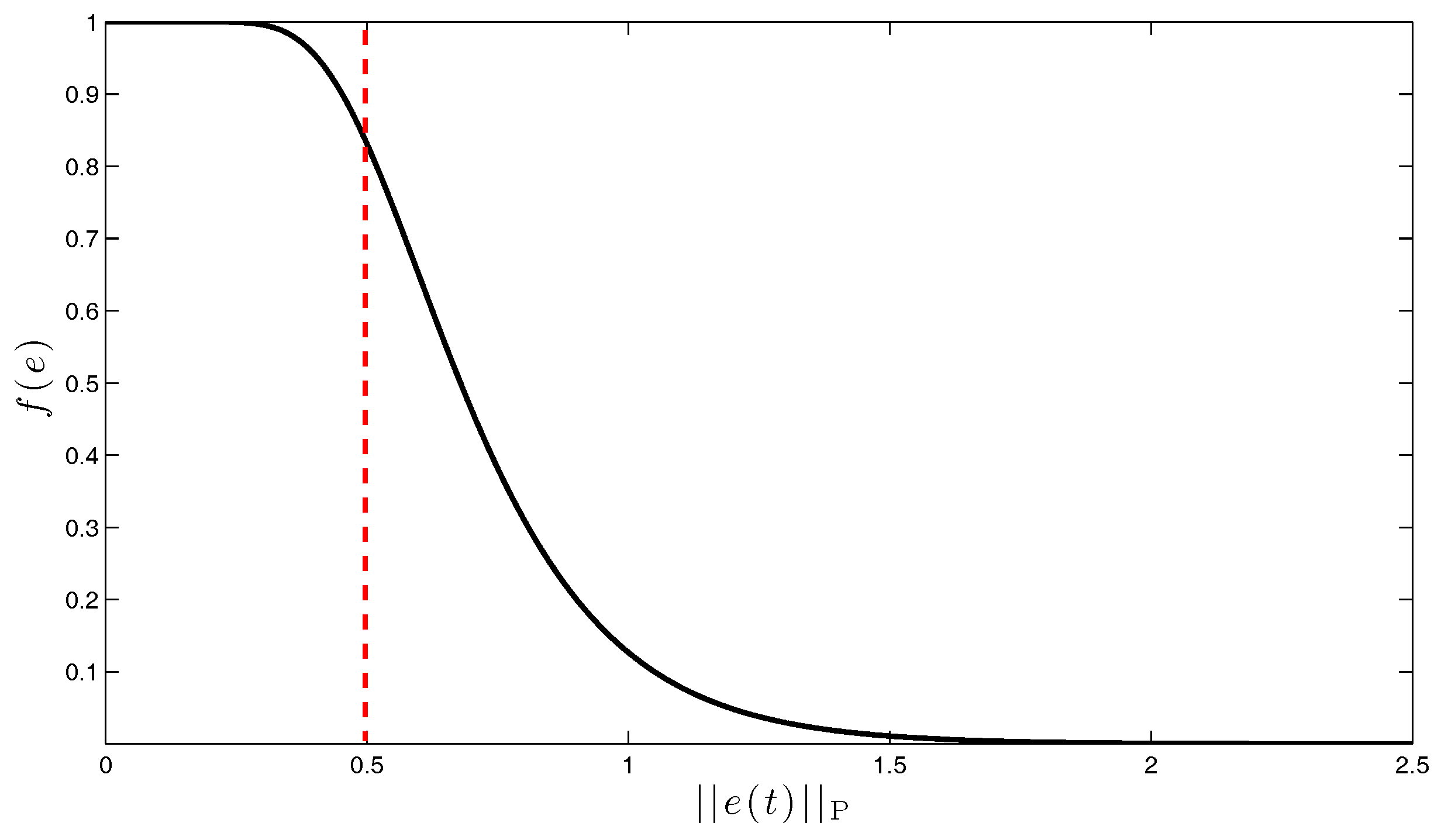
3. Direct Uncertainty Minimization for Adaptive System Performance Improvement: Linear Reference Model Case

For the model reference adaptive control framework introduced in Section 2, we now develop the direct uncertainty minimization mechanism to improve transient system response. In particular, we first modify the adaptive feedback control law given by Equation (13) as:

$$\begin{array}{c}\hfill u_{\mathrm{a}}\left(t\right)=-{\widehat{W}}^{\mathrm{T}}\left(t\right)\sigma \left(x\left(t\right)\right)-\varphi \left(t\right),\end{array}$$

(25)

where $\varphi \left(t\right)\in {\mathbb{R}}^m$ is the system performance improvement term that satisfies:

$$\begin{array}{ccc}\hfill \varphi \left(t\right)& =& \varphi \left(0\right)+k{\left(B^{\mathrm{T}}B\right)}^{-1}{B}^{\mathrm{T}}\left[\right(e\left(t\right)-e\left(0\right))-{\int }_0^t{A}_{\mathrm{r}}e\left(\tau \right)\mathrm{d}\tau ],\hfill \end{array}$$

(26)

with $k\in {\mathbb{R}}_{+}$ being a design parameter. Using Equation (25), the system error dynamics in Equation (18) become:

$$\begin{array}{ccc}\hfill \dot{e}\left(t\right)& =& A_{\mathrm{r}}e\left(t\right)-B\Lambda [{\tilde{W}}^{\mathrm{T}}\left(t\right)\sigma \left(x\left(t\right)\right)+\varphi \left(t\right)],e\left(0\right)=e_0.\hfill \end{array}$$

(27)

Notice that the ideal system error dynamics have the form:

$$\begin{array}{ccc}\hfill \dot{e}\left(t\right)& =& A_{\mathrm{r}}e\left(t\right),e\left(0\right)=e_0,\hfill \end{array}$$

(28)

under nominal conditions with $\varphi \left(t\right)\equiv 0$ when there is no system uncertainty or control uncertainty. Motivating from this standpoint, the mismatch term ${\tilde{W}}^{\mathrm{T}}\left(t\right)\sigma \left(x\left(t\right)\right)+\varphi \left(t\right)$ in Equation (27) has to be minimized during the transient system response to improve system performance. In the next theorem, we show that the proposed system performance improvement term given by Equation (26) achieves this objective through a gradient minimization procedure.

Theorem 1.

The modification term of the adaptive feedback control law in Equation (26) is the negative gradient of the cost function given by:

$$\begin{array}{ccc}\hfill \mathcal{J}(·)& =& \frac{k}{2}||{\Lambda }^{1/2}({\tilde{W}}^{\mathrm{T}}\left(t\right)\sigma \left(x\left(t\right)\right)+\varphi \left(t\right))|{|}_2^2.\hfill \end{array}$$

(29)

Proof. 

The negative gradient of the cost function given by Equation (29) with respect to $\varphi \left(t\right)$ has the form given by:

$$\begin{array}{ccc}\hfill -\frac{\partial \mathcal{J}(·)}{\partial \varphi \left(t\right)}& =& -k[\Lambda ({\tilde{W}}^{\mathrm{T}}\left(t\right)\sigma \left(x\left(t\right)\right)+\varphi \left(t\right))],\hfill \end{array}$$

(30)

which can be rewritten using Equation (27) as:

$$\begin{array}{ccc}\hfill -\frac{\partial \mathcal{J}(·)}{\partial \varphi \left(t\right)}& =& k{\left(B^{\mathrm{T}}B\right)}^{-1}{B}^{\mathrm{T}}[\dot{e}\left(t\right)-A_{\mathrm{r}}e\left(t\right)].\hfill \end{array}$$

(31)

In Equation (31), note that $B^{\mathrm{T}}B=B_{\mathrm{p}}^{\mathrm{T}}{B}_{\mathrm{p}}$ is nonsingular by its definition in Section 2. To construct the modification term of the adaptive feedback control law in Equation (26), let:

$$\begin{array}{ccc}\hfill \dot{\varphi }\left(t\right)& =& -\frac{\partial \mathcal{J}(·)}{\partial \varphi \left(t\right)}\hfill \\ & =& k{\left(B^{\mathrm{T}}B\right)}^{-1}{B}^{\mathrm{T}}[\dot{e}\left(t\right)-A_{\mathrm{r}}e\left(t\right)],\hfill \end{array}$$

(32)

where Equation (26) is a direct consequence of Equation (32) using integration by parts. ☐

Remark 3.

The proposed modification term of the adaptive feedback control law in Equation (26) allows for the system error to be shaped by suppressing the mismatch term ${\tilde{W}}^{\mathrm{T}}\left(t\right)\sigma \left(x\left(t\right)\right)+\varphi \left(t\right)$ in Equation (27) due to gradient minimization, since it is constructed to be the negative gradient of Equation (29) with respect to $\varphi \left(t\right)$. Therefore, by adjusting k in Equation (26), the uncertain dynamical system response and the reference model response can be made close to each other for all time including the transient phase. See Section 5 for illustrative numerical examples.

Next, to maintain closed-loop system stability under the modified adaptive control signal given by Equation (25), we now modify the update law given by Equation (14) as:

$$\begin{array}{ccc}\hfill \dot{\widehat{W}}\left(t\right)& =& \gamma \sigma \left(x\left(t\right)\right)[e^{\mathrm{T}}\left(t\right)PB+\xi {\varphi }^{\mathrm{T}}\left(t\right)],\widehat{W}\left(0\right)={\widehat{W}}_0,\hfill \end{array}$$

(33)

with $\xi =k/a$ and $a\in {\mathbb{R}}_{+}$ being a design parameter.

Remark 4.

Note that the structure of Equation (26) is much simpler than the structure of (44) in [11], in that the former does not involve $\widehat{W}\left(t\right)$ dependence and additional integration terms. Furthermore, the same conclusion is also true when Equation (33) is compared with (31)–(33) of [11], where the latter has an extra differential equation in addition to the modification terms. Thus, the approach proposed here is much less computationally expensive than [9,10,11].

Now, we are ready to state the following theorem, which shows the asymptotic stability of the pair $\left(e\right(t),\varphi (t\left)\right)$, as well as the Lyapunov stability of $\tilde{W}\left(t\right)$.

Theorem 2.

Consider the uncertain dynamical system given by Equation (1) subject to Assumption 1, the reference model given by Equation (15) and the feedback control law given by Equation (25) with Equations (26) and (33). In addition, let ξ be chosen such that:

$$\begin{array}{c}\hfill {\lambda }_{\min }\left(R\right)-\frac{1}{\xi }||PB|{|}_{\mathrm{F}}^2{\Lambda }^{*}>0\end{array}$$

(34)

holds, where $\left|\right|\Lambda |{|}_{\mathrm{F}}\le {\Lambda }^{*}$ (here, ${\Lambda }^{*}\in {\mathbb{R}}_{+}$ is a known, possibly conservative bound on the control effectiveness). Then, the solution $(e\left(t\right),\varphi \left(t\right),\tilde{W}\left(t\right))$ of the closed-loop dynamical system is Lyapunov stable for all initial conditions and $t\in {\overline{\mathbb{R}}}_{+}$, ${lim}_{t\to \infty }e\left(t\right)=0$ and ${lim}_{t\to \infty }\varphi \left(t\right)=0$.

Proof. 

To show Lyapunov stability of the solution $(e\left(t\right),\varphi \left(t\right),\tilde{W}\left(t\right))$, consider the Lyapunov function candidate given by:

$$\begin{array}{ccc}\hfill \mathcal{V}(e,\varphi ,\tilde{W})& =& e^{\mathrm{T}}Pe+a^{-1}{\varphi }^{\mathrm{T}}\varphi +{\gamma }^{-1}\mathrm{tr}{(\tilde{W}{\Lambda }^{1/2})}^{\mathrm{T}}(\tilde{W}{\Lambda }^{1/2}).\hfill \end{array}$$

(35)

Note that $\mathcal{V}(0,0,0)=0$ and $\mathcal{V}(e,\varphi ,\tilde{W})>0$ for all $(e,\varphi ,\tilde{W})\ne (0,0,0)$. Differentiating Equation (35) along the closed-loop dynamical system trajectories yields:

$$\begin{array}{ccc}\hfill \dot{\mathcal{V}}(e\left(t\right),\varphi \left(t\right),\tilde{W}\left(t\right))& =& -e^{\mathrm{T}}\left(t\right)Re\left(t\right)-2\xi {\varphi }^{\mathrm{T}}\left(t\right)\Lambda \varphi \left(t\right)-2e^{\mathrm{T}}\left(t\right)PB{\Lambda }^{1/2}{\Lambda }^{1/2}\varphi \left(t\right).\hfill \end{array}$$

(36)

Using Young’s inequality [21] for the last term in Equation (36) gives:

$$\begin{array}{cc}\hfill -2e^{\mathrm{T}}\left(t\right)PB{\Lambda }^{1/2}{\Lambda }^{1/2}\varphi \left(t\right)\le & |-2e^{\mathrm{T}}\left(t\right)PB{\Lambda }^{1/2}{\Lambda }^{1/2}\varphi \left(t\right)|\hfill \\ \hfill \le & \frac{1}{\mu }{e}^{\mathrm{T}}\left(t\right)PB\Lambda B^{\mathrm{T}}Pe\left(t\right)+\mu {\varphi }^{\mathrm{T}}\left(t\right)\Lambda \varphi \left(t\right).\hfill \end{array}$$

(37)

Now, setting $\mu =\xi$ and using Equation (37) in Equation (36) yields:

$$\begin{array}{cc}\hfill \dot{\mathcal{V}}(e\left(t\right),\varphi \left(t\right),\tilde{W}\left(t\right))\le & -e^{\mathrm{T}}\left(t\right)Re\left(t\right)+\frac{1}{\xi }{e}^{\mathrm{T}}\left(t\right)PB\Lambda B^{\mathrm{T}}Pe\left(t\right)-\xi {\varphi }^{\mathrm{T}}\left(t\right)\Lambda \varphi \left(t\right)\hfill \\ \hfill \le & -{\lambda }_{\min }\left(R\right)||e\left(t\right)|{|}_2^2+\frac{1}{\xi }||e\left(t\right)|{|}_2^2||PB|{|}_{\mathrm{F}}^2{\Lambda }^{*}-\xi {\lambda }_{\min }(\Lambda )||\varphi \left(t\right)|{|}_2^2\hfill \\ \hfill =& -||e\left(t\right)|{|}_2^2[{\lambda }_{\min }\left(R\right)-\frac{1}{\xi }||PB|{|}_{\mathrm{F}}^2{\Lambda }^{*}]-\xi {\lambda }_{\min }(\Lambda )||\varphi \left(t\right)|{|}_2^2\hfill \end{array}$$

(38)

Using the condition Equation (34) in Equation (38), it follows that $\dot{\mathcal{V}}(e\left(t\right),\varphi \left(t\right),\tilde{W}\left(t\right))\le 0$, which guarantees the Lyapunov stability of the solution $(e\left(t\right),\varphi \left(t\right),\tilde{W}\left(t\right))$. Since this implies the boundedness of $e\left(t\right)$, $\varphi \left(t\right)$ and $\tilde{W}\left(t\right)$ for all $t\in {\overline{\mathbb{R}}}_{+}$, it follows from Equation (27) and Equation (32) that $\dot{e}\left(t\right)$ and $\dot{\varphi }\left(t\right)$ are bounded for all $t\in {\overline{\mathbb{R}}}_{+}$, and hence, $\ddot{\mathcal{V}}(e\left(t\right),\varphi \left(t\right),\tilde{W}\left(t\right))$ is bounded for all $t\in {\overline{\mathbb{R}}}_{+}$. It now follow from Barbalat’s lemma [17]:

$$\begin{array}{ccc}\hfill \underset{t\to \infty }{lim}\dot{\mathcal{V}}(e\left(t\right),\varphi \left(t\right),\tilde{W}\left(t\right))& =& 0,\hfill \end{array}$$

(39)

which shows that ${lim}_{t\to \infty }e\left(t\right)=0$ and ${lim}_{t\to \infty }\varphi \left(t\right)=0$. ☐

From a practical standpoint, if $e\left(t\right)$ is sufficiently small, then the design parameter ξ, which affects both modification terms in Equations (25) and (33), can be chosen to be small, such that Equation (34) holds. However, as $e\left(t\right)$ becomes large, then ξ may need to be increased accordingly to put more weight on minimizing the cost function given by Equation (29) and, hence, to enforce system error to approximately stay in a priori given, user-defined performance bounds. To achieve this practical objective, we can let $\xi \left(t\right)=k\left(t\right)/a$, where $\xi \left(t\right)\in [{\xi }_{\min },{\xi }_{\max }]$, ${\xi }_{\min }\in {\mathbb{R}}_{+}$, ${\xi }_{\max }\in {\mathbb{R}}_{+}$, and consider the cost function given by:

$$\begin{array}{ccc}\hfill \mathcal{J}(·)& =& \frac{k\left(t\right)}{2}||{\Lambda }^{1/2}({\tilde{W}}^{\mathrm{T}}(t)\sigma (x\left(t\right))+\varphi \left(t\right))|{|}_2^2.\hfill \end{array}$$

(40)

Choosing the modification term in Equation (25) as the negative gradient of Equation (40), i.e., $\dot{\varphi }\left(t\right)=-\frac{\partial \mathcal{J}(·)}{\partial \varphi \left(t\right)}$, and following similar steps as highlighted in the proof of Theorem 1, it follows by integration by parts that:

$$\begin{array}{cc}\hfill \varphi \left(t\right)=& \varphi \left(0\right)+a[\xi \left(t\right){\left(B^{\mathrm{T}}B\right)}^{-1}{B}^{\mathrm{T}}e\left(t\right)-\xi \left(0\right){\left(B^{\mathrm{T}}B\right)}^{-1}{B}^{\mathrm{T}}e\left(0\right)-{\int }_0^t\dot{\xi }\left(\tau \right){\left(B^{\mathrm{T}}B\right)}^{-1}{B}^{\mathrm{T}}e\left(\tau \right)\mathrm{d}\tau \hfill \\ & -{\int }_0^t\xi \left(\tau \right){\left(B^{\mathrm{T}}B\right)}^{-1}{B}^{\mathrm{T}}{A}_{\mathrm{r}}e\left(\tau \right)\mathrm{d}\tau ].\hfill \end{array}$$

(41)

Notice that in this case, the modified update law becomes:

$$\begin{array}{ccc}\hfill \dot{\widehat{W}}\left(t\right)& =& \gamma \sigma \left(x\left(t\right)\right)[e^{\mathrm{T}}\left(t\right)PB+\xi \left(t\right){\varphi }^{\mathrm{T}}\left(t\right)],\widehat{W}\left(0\right)={\widehat{W}}_0,\hfill \end{array}$$

(42)

and the condition Equation (34) needs to be replaced with:

$$\begin{array}{c}\hfill {\lambda }_{\min }\left(R\right)-\frac{1}{{\xi }_{\min }}||PB|{|}_{\mathrm{F}}^2{\Lambda }^{*}>0,\end{array}$$

(43)

where $\left|\right|\Lambda |{|}_{\mathrm{F}}\le {\Lambda }^{*}$ (here, ${\Lambda }^{*}\in {\mathbb{R}}_{+}$ is a known bound on the control effectiveness). In addition, we choose:

$$\begin{array}{ccc}\hfill \dot{\xi }\left(t\right)& =& -{\gamma }_{\xi }\left[f\left(e\right)\right(\xi \left(t\right)-{\xi }_{\min })+(1-f\left(e\right)\left)\right(\xi \left(t\right)-{\xi }_{\max }\left)\right],\xi \left(0\right)={\xi }_0\in [{\xi }_{\min },{\xi }_{\max }],\hfill \end{array}$$

(44)

where ${\gamma }_{\xi }\in {\mathbb{R}}_{+}$ and $f\left(e\right)\in [0,1]$ is a continuously differentiable function, such that it is close to one when $e\left(t\right)$ is sufficiently small and otherwise close to zero. It follows from Equation (44) that $\xi \left(t\right)\in [{\xi }_{\min },{\xi }_{\max }]$ and $\xi \left(t\right)$ approach to ${\xi }_{\min }$ (resp., ${\xi }_{\max }$) when $f\left(e\right)=1$ (resp., $f\left(e\right)=0$). A candidate $f\left(e\right)$ has the form $f\left(e\right)=1-[1-\mathrm{sech}(c_1{\left|\right|e\left(t\right)\left|\right|}_{\mathrm{P}}){]}^{c_2}$, ${\left|\right|e\left(t\right)\left|\right|}_{\mathrm{P}}\triangleq \sqrt{e^{\mathrm{T}}\left(t\right)Pe\left(t\right)}$, where it is depicted in Figure 1 for $c_1=5$ (this is chosen to drive $\xi \left(t\right)$ to ${\xi }_{\max }$ if ${\left|\right|e\left(t\right)\left|\right|}_{\mathrm{P}}$ is larger than 0.5) and $c_2=10$.

4. Generalization to a Class of Nonlinear Reference Models

In most of the model reference adaptive control literature, it is common to design a reference model with linear dynamics as given by Equation (15). While this is practical for several applications, the control designer may prefer to use a nonlinear reference model to better capture the desired closed-loop system performance for many robotics and flight control applications. By adopting the tools and methods from [12,13], we now generalize the results in Section 3 such that the proposed direct uncertainty minimization adaptive control architecture can be used to suppress the effect of the system uncertainty on the transient system response and drive the states of a nonlinear uncertain dynamical system to the states of a class of nonlinear reference models.

For this purpose, we recast the uncertain dynamical system given by Equation (1) with a more general class of affine-in-control nonlinear system dynamics given by:

$$\begin{array}{ccc}\hfill {\dot{x}}_{\mathrm{p}}\left(t\right)& =& f_{\mathrm{p}}\left(x_{\mathrm{p}}\left(t\right)\right)+B_{\mathrm{p}}\Lambda u\left(t\right)+B_{\mathrm{p}}{\delta }_{\mathrm{p}}\left(x_{\mathrm{p}}\left(t\right)\right),x_{\mathrm{p}}\left(0\right)=x_{{}_{\mathrm{p}}0},\hfill \end{array}$$

(45)

where $x_{\mathrm{p}}\left(t\right)\in {\mathbb{R}}^{n_{\mathrm{p}}}$ is the state vector, $u\left(t\right)\in {\mathbb{R}}^m$ is the control input restricted to the class of admissible controls consisting of measurable functions such that $f_{\mathrm{p}}:{\mathbb{R}}^{n_{\mathrm{p}}}\to {\mathbb{R}}^{n_{\mathrm{p}}}$ is a known system function that satisfies $f_{\mathrm{p}}\left(0\right)=0$, $B_{\mathrm{p}}\in {\mathbb{R}}^{n_{\mathrm{p}}\times m}$ is a known control input matrix, $\Lambda \in {\mathbb{R}}_{+}^{m\times m}\cap {\mathbb{D}}^{m\times m}$ is an unknown control effectiveness matrix and ${\delta }_{\mathrm{p}}:{\mathbb{R}}^{n_{\mathrm{p}}}\to {\mathbb{R}}^m$ is the system uncertainty, and it is implicitly assumed that the required properties for the existence and uniqueness of solutions are satisfied for the controllable uncertain dynamical system, such that Equation (45) has a unique solution forward in time [17,22].

Once again, to address the command following, Equation (45) can be augmented with the integrator state dynamics given by Equation (3) in the following form subject to Assumption 1:

$$\begin{array}{ccc}\hfill \dot{x}\left(t\right)& =& f(x\left(t\right),c\left(t\right))+B\Lambda u\left(t\right)+B{W}_{\mathrm{p}}^{\mathrm{T}}{\sigma }_{\mathrm{p}}\left(x_{\mathrm{p}}\left(t\right)\right),x\left(0\right)=x_0,\hfill \end{array}$$

(46)

where $x\left(t\right)\triangleq {[x_{\mathrm{p}}^{\mathrm{T}}\left(t\right),x_{\mathrm{c}}^{\mathrm{T}}\left(t\right)]}^{\mathrm{T}}\in {\mathbb{R}}^n$, $n=n_{\mathrm{p}}+n_{\mathrm{c}}$, is the augmented state vector, $x_0={[x_{\mathrm{p}0}^{\mathrm{T}},x_{\mathrm{c}0}^{\mathrm{T}}]}^{\mathrm{T}}\in {\mathbb{R}}^n$, $c\left(t\right)\in {\mathbb{R}}^{n_{\mathrm{c}}}$ is a given bounded command, B is given by Equation (6) and $f:{\mathbb{R}}^n\times {\mathbb{R}}^{n_{\mathrm{c}}}\to {\mathbb{R}}^n$ is the aggregated system function with the integrator state dynamics that satisfies $f(0,0)=0$ and:

$$\begin{array}{ccc}\hfill f\left(x\right(t),c(t\left)\right)& =& \left[\begin{array}{c}{f}_{\mathrm{p}}\left(x_{\mathrm{p}}\left(t\right)\right)\\ E_{\mathrm{p}}{x}_{\mathrm{p}}\left(t\right)-c\left(t\right)\end{array}\right].\hfill \end{array}$$

(47)

Next, consider the nonlinear reference model given by:

$$\begin{array}{ccc}\hfill {\dot{x}}_{\mathrm{r}}\left(t\right)& =& f_{\mathrm{r}}(x_{\mathrm{r}}\left(t\right),c\left(t\right)),x_{\mathrm{r}}\left(0\right)=x_{\mathrm{r}0},\hfill \end{array}$$

(48)

where $x_{\mathrm{r}}\left(t\right)\in {\mathbb{R}}^n$ is the reference state vector and $f_{\mathrm{r}}:{\mathbb{R}}^n\times {\mathbb{R}}^{n_{\mathrm{c}}}\to {\mathbb{R}}^n$ is the reference model function that satisfies $f_{\mathrm{r}}(0,0)=0$ and:

$$\begin{array}{ccc}\hfill f_{\mathrm{r}}(x_{\mathrm{r}}\left(t\right),c\left(t\right))& \triangleq & f(x_{\mathrm{r}}\left(t\right),c\left(t\right))-Bk\left(x_{\mathrm{r}}\left(t\right)\right),\hfill \end{array}$$

(49)

with $k:{\mathbb{R}}^n\to {\mathbb{R}}^m$ being a feedback law such that $x_{\mathrm{r}}\left(t\right)$ is bounded for all $t\in {\overline{\mathbb{R}}}_{+}$. In addition, it is implicitly assumed that Equation (48) has a unique solution forward in time.

Let the nominal control law be given by:

$$\begin{array}{ccc}\hfill u_{\mathrm{n}}\left(t\right)& =& -k\left(x\right(t\left)\right),\hfill \end{array}$$

(50)

such that with Equation (8), Equation (46) can be rewritten as:

$$\begin{array}{cc}\hfill \dot{x}\left(t\right)=& f(x\left(t\right),c\left(t\right))-Bk\left(x\left(t\right)\right)+B\Lambda [u_{\mathrm{a}}\left(t\right)+{\Lambda }^{-1}{W}_{\mathrm{p}}^{\mathrm{T}}{\sigma }_{\mathrm{p}}\left(x_{\mathrm{p}}\left(t\right)\right)+({\Lambda }^{-1}-I)k\left(x\left(t\right)\right)]\hfill \\ \hfill =& f_{\mathrm{r}}(x\left(t\right),c\left(t\right))+B\Lambda [u_{\mathrm{a}}\left(t\right)+W_{\mathrm{o}}^{\mathrm{T}}{\sigma }_{\mathrm{o}}\left(x\left(t\right)\right)],\hfill \end{array}$$

(51)

where $W_{\mathrm{o}}\triangleq {[{\Lambda }^{-1}{W}_{\mathrm{p}}^{\mathrm{T}},({\Lambda }^{-1}-I)]}^{\mathrm{T}}\in {\mathbb{R}}^{(s+m)\times m}$ and ${\sigma }_{\mathrm{o}}\left(x\left(t\right)\right)\triangleq {[{\sigma }_{\mathrm{p}}^{\mathrm{T}}\left(x_{\mathrm{p}}\left(t\right)\right),k^{\mathrm{T}}\left(x\left(t\right)\right)]}^{\mathrm{T}}\in {\mathbb{R}}^{(s+m)}$. The system error dynamics then follow from Equations (48) and (51) as:

$$\begin{array}{ccc}\hfill \dot{e}\left(t\right)& =& f_{\mathrm{r}}(x\left(t\right),c\left(t\right))-f_{\mathrm{r}}(x_{\mathrm{r}}\left(t\right),c\left(t\right))+B\Lambda [u_{\mathrm{a}}\left(t\right)+W_{\mathrm{o}}^{\mathrm{T}}{\sigma }_{\mathrm{o}}\left(x\left(t\right)\right)],e\left(0\right)=e_0.\hfill \end{array}$$

(52)

Note that there exists a known signal $v(x\left(t\right),x_{\mathrm{r}}\left(t\right),c\left(t\right))\in {\mathbb{R}}^m$, which can be used as a feedback linearization term, such that:

$$\begin{array}{c}\hfill A_{\mathrm{r}}e\left(t\right)=f_{\mathrm{r}}(x\left(t\right),c\left(t\right))-f_{\mathrm{r}}(x_{\mathrm{r}}\left(t\right),c\left(t\right))+Bv(·)\end{array}$$

(53)

holds, and hence, Equation (52) can be written as:

$$\begin{array}{ccc}\hfill \dot{e}\left(t\right)& =& A_{\mathrm{r}}e\left(t\right)+B\Lambda [u_{\mathrm{a}}\left(t\right)+W_{\mathrm{o}}^{\mathrm{T}}{\sigma }_{\mathrm{o}}\left(x\left(t\right)\right)-{\Lambda }^{-1}v(·)]\hfill \\ & =& A_{\mathrm{r}}e\left(t\right)+B\Lambda [u_{\mathrm{a}}\left(t\right)+W^{\mathrm{T}}\sigma (·)],\hfill \end{array}$$

(54)

with $W\triangleq {[W_{\mathrm{o}}^{\mathrm{T}},-{\Lambda }^{-1}]}^{\mathrm{T}}\in {\mathbb{R}}^{(s+2m)\times m}$ being the unknown aggregated weight matrix and $\sigma (·)\triangleq {[{\sigma }_{\mathrm{o}}^{\mathrm{T}}\left(x\left(t\right)\right),v^{\mathrm{T}}(·)]}^{\mathrm{T}}\in {\mathbb{R}}^{(s+2m)}$ being the known aggregated basis function.

Now, consider the adaptive feedback control law given by:

$$\begin{array}{c}\hfill u_{\mathrm{a}}\left(t\right)=-{\widehat{W}}^{\mathrm{T}}\left(t\right)\sigma (·)-\varphi \left(t\right),\end{array}$$

(55)

where $\varphi \left(t\right)\in {\mathbb{R}}^m$ satisfies Equation (41) with Equation (44) and $\widehat{W}\left(t\right)\in {\mathbb{R}}^{(s+2m)\times m}$ satisfies:

$$\begin{array}{ccc}\hfill \dot{\widehat{W}}\left(t\right)& =& \gamma \sigma (·)[e^{\mathrm{T}}\left(t\right)PB+\xi \left(t\right){\varphi }^{\mathrm{T}}\left(t\right)],\widehat{W}\left(0\right)={\widehat{W}}_0.\hfill \end{array}$$

(56)

Using Equation (55) in Equation (54), it follows that the system error dynamics can be written as:

$$\begin{array}{ccc}\hfill \dot{e}\left(t\right)& =& A_{\mathrm{r}}e\left(t\right)-B\Lambda [{\tilde{W}}^{\mathrm{T}}\left(t\right)\sigma (·)+\varphi \left(t\right)],\hfill \end{array}$$

(57)

where $\tilde{W}\left(t\right)\triangleq \widehat{W}\left(t\right)-W\in {\mathbb{R}}^{(s+2m)\times m}$.

Remark 5.

It should be noted that the term $v(·)$ acts similar to a feedback linearization signal, which is an important feature in generalizing the direct uncertainty minimization framework for the considered class of nonlinear reference models. By appropriately selecting $v(·)$, when possible, for the given application, such that Equation (53) holds, and then embedding $v(·)$ into the unknown weight matrix W and the known basis function $\sigma (·)$, the resulting system error dynamics given by Equation (57) has an identical structure to the system error dynamics given by Equation (27) in Section 3 for the linear reference model. It then follows that the analysis and synthesis of the direct uncertainty minimization mechanism and stability analysis presented in Section 3 directly translates to the case in which nonlinear reference models are used.

Theorem 3.

Consider the nonlinear uncertain dynamical system given by Equation (45) subject to Assumption 1; the nonlinear reference model given by Equation (48) and the feedback control law given by Equation (55) with Equations (41), (44) and (56). In addition, let ${\xi }_{\min }$ be chosen, such that Equation (43) holds. Then, the solution $(e\left(t\right),\varphi \left(t\right),\tilde{W}\left(t\right))$ of the closed-loop dynamical system is Lyapunov stable for all initial conditions, and $t\in {\overline{\mathbb{R}}}_{+}$, ${lim}_{t\to \infty }e\left(t\right)=0$ and ${lim}_{t\to \infty }\varphi \left(t\right)=0$.

Proof. 

As a consequence of the discussion highlighted in Remark 5, the proof is similar to the proof of Theorem 2, and hence, is omitted. ☐

5. Illustrative Numerical Examples

To demonstrate the efficacy of the proposed direct uncertainty minimization framework, we now present two examples in the following two subsections. We first investigate the application to a hypersonic vehicle using a linear reference model. The second example considers a wing rock dynamics model for an aircraft with a nonlinear reference model, where the purpose of the nonlinear reference model is to limit the pilot authority for envelope protection.

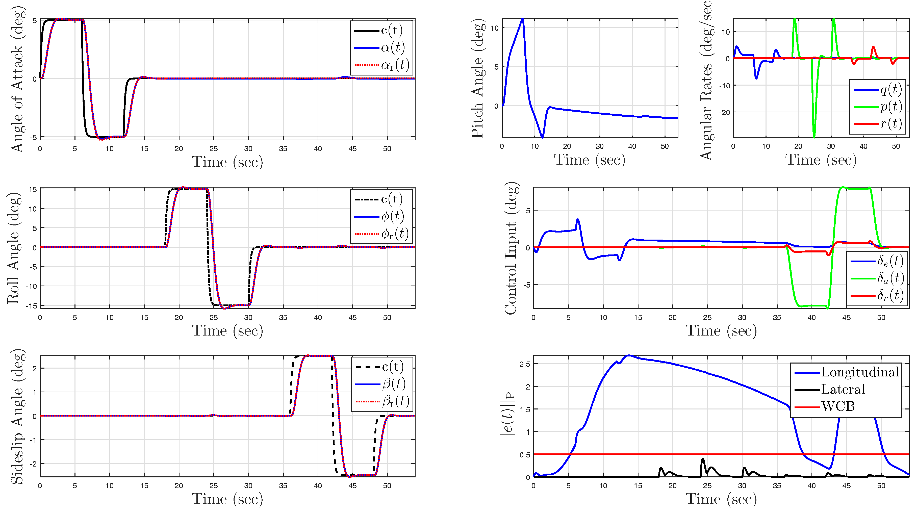
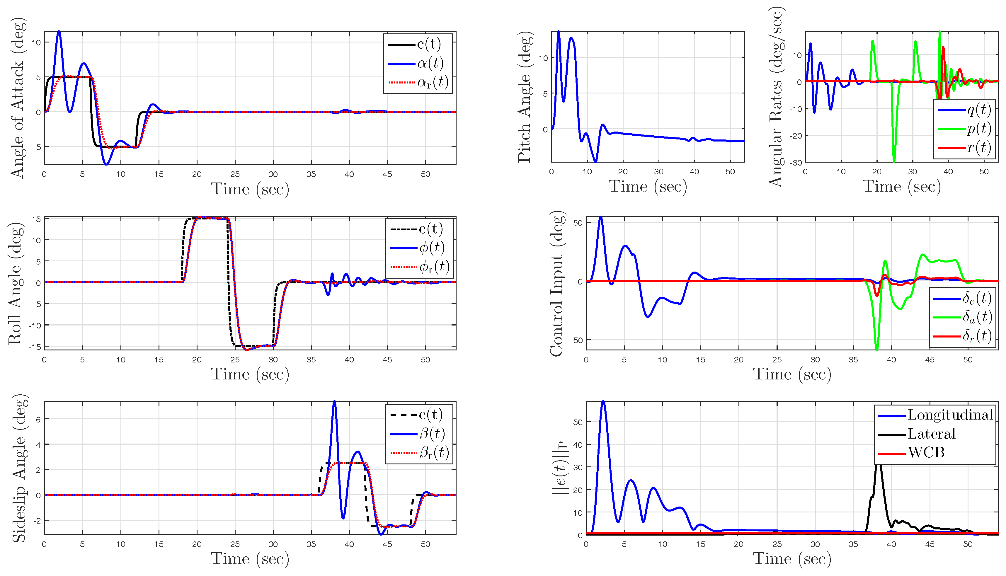
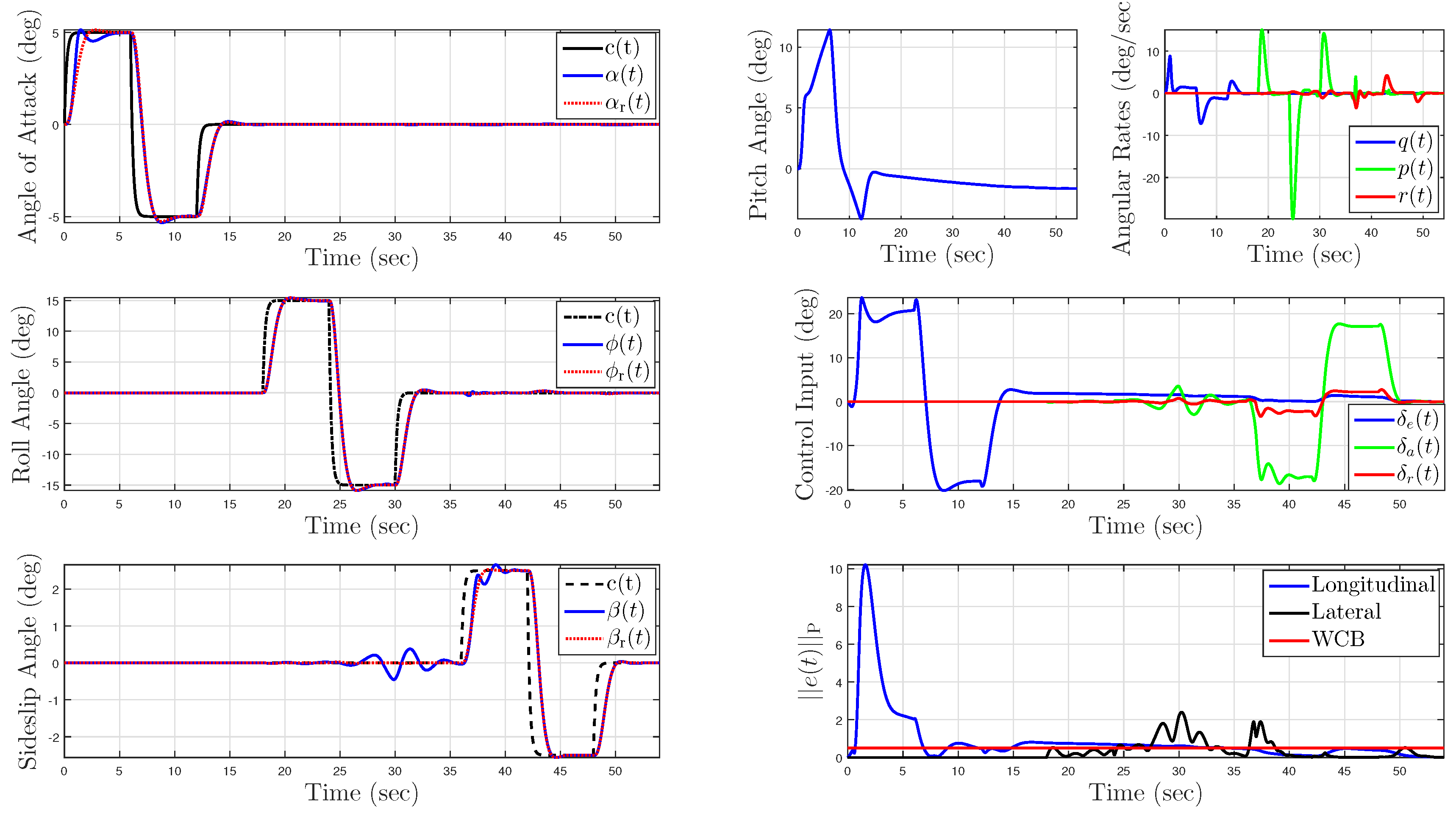
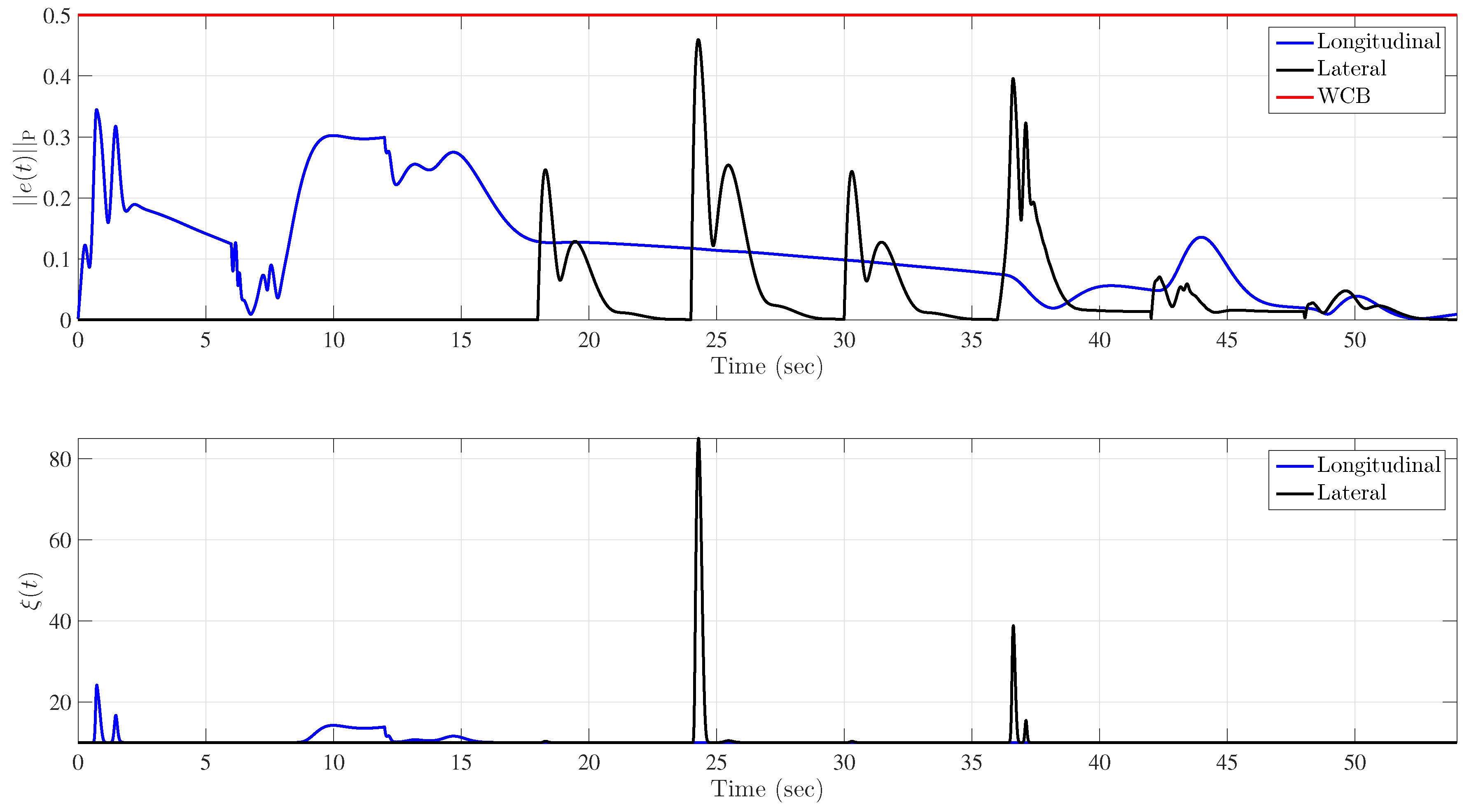
5.1. Example 1: Application to a Hypersonic Vehicle Model

For this example, we first formulate a state space model of a generic hypersonic vehicle (GHV). Then, it is explained how the model is decoupled into longitudinal and lateral dynamics for which separate controllers are designed. The longitudinal and lateral controllers have both a nominal and adaptive portion where the simulation results illustrate both nominal control performance, a standard adaptive control performance and the proposed adaptive control performance.

For the configuration with an altitude of 80,000 feet and a Mach number of six, a linearized model under nominal conditions $({\delta }_{\mathrm{p}}\left(x_{\mathrm{p}}\left(t\right)\right)=0\mathrm{and}\Lambda =I)$ is obtained in the form of Equation (1) with:

$$\begin{array}{r}\hfill \begin{array}{c}\hfill A_{\mathrm{p}}=\left[\begin{array}{ccccc}-3.70\times {10}^{-3}& -7.17\times {10}^{-1}& 0& -3.18\times {10}^1& -2.67\times {10}^{-4}\\ -5.35\times {10}^{-7}& -2.39\times {10}^{-1}& 1& -2.95\times {10}^{-12}& 2.23\times {10}^{-7}\\ -2.79\times {10}^{-5}& 4.26& -1.19\times {10}^{-1}& 0& 3.94\times {10}^{-5}\\ -4.76\times {10}^{-8}& 1.31\times {10}^{-13}& 1& -4.45\times {10}^{-14}& -1.33\times {10}^{-11}\\ -5.53\times {10}^{-10}& -5.87\times {10}^3& 0& 5.87\times {10}^3& 0\\ 5.99\times {10}^{-16}& -3.14\times {10}^{-11}& 0& -3.04\times {10}^{-19}& -9.74\times {10}^{-16}\\ 1.47\times {10}^{-10}& -4.45\times {10}^{-6}& 0& 0& -1.00\times {10}^{-11}\\ -5.29\times {10}^{-12}& 3.98\times {10}^{-8}& 0& 0& 1.28\times {10}^{-12}\\ 8.08\times {10}^{-28}& 2.04\times {10}^{-22}& 1.01\times {10}^{-20}& 1.17\times {10}^{-16}& -1.73\times {10}^{-31}\end{array}\right.\cdots \end{array}\\ \hfill \cdots \left.\begin{array}{ccccc}& -8.81\times {10}^{-1}& 0& 0& -1.77\times {10}^{-15}\\ & -1.06\times {10}^{-3}& 0& 0& -3.18\times {10}^{-21}\\ & -1.47& 0& 0& 0\\ & -1.08\times {10}^{-19}& 4.44\times {10}^{-16}& -9.58\times {10}^{-16}& -2.58\times {10}^{-18}\\ & 0& 0& 0& -3.26\times {10}^{-13}\\ & -6.97\times {10}^{-2}& -1.04\times {10}^{-2}& -9.99\times {10}^{-1}& -5.35\times {10}^{-3}\\ & -1.31\times {10}^3& -2.03& -7.54\times {10}^{-3}& 0\\ & 2.07& -1.55\times {10}^{-3}& -5.31\times {10}^{-2}& 0\\ & -2.38\times {10}^{-4}& 8.54\times {10}^{-1}& -8.84\times {10}^{-3}& -3.00\times {10}^{-6}\end{array}\right]\end{array}$$

(58)

$$B_{\mathrm{p}}=\left[\begin{array}{ccc}-6.53\times {10}^{-3}& -1.24\times {10}^{-13}& -2.98\times {10}^{-3}\\ -1.33\times {10}^{-4}& -2.44\times {10}^{-13}& 1.17\times {10}^{-7}\\ -1.84\times {10}^{-1}& -1.60\times {10}^{-13}& 2.48\times {10}^{-4}\\ 0& 0& 0\\ 0& 0& 0\\ -1.40\times {10}^{-16}& -2.47\times {10}^{-5}& -2.18\times {10}^{-4}\\ -5.90\times {10}^{-11}& -8.04& 10.3\\ 8.56\times {10}^{-14}& 3.17\times {10}^{-2}& 2.85\times {10}^{-1}\\ 0& 0& 0\end{array}\right]$$

(59)

with the state vector being defined as $x_{\mathrm{p}}\left(t\right)={[V\left(t\right),\alpha \left(t\right),q\left(t\right),\theta \left(t\right),h\left(t\right),\beta \left(t\right),p\left(t\right),r\left(t\right),\varphi \left(t\right)]}^{\mathrm{T}}$, where $V\left(t\right)$ denotes the total velocity, $\alpha \left(t\right)$ denotes the angle of attack, $q\left(t\right)$ denotes the pitch rate, $\theta \left(t\right)$ denotes the pitch angle, $h\left(t\right)$ denotes the altitude, $\beta \left(t\right)$ denotes the sideslip angle, $p\left(t\right)$ denotes the roll rate, $r\left(t\right)$ denotes the yaw rate and $\varphi \left(t\right)$ denotes the roll angle. The control input vector is defined as $u\left(t\right)={[{\delta }_{\mathrm{e}}\left(t\right),{\delta }_{\mathrm{a}}\left(t\right),{\delta }_{\mathrm{r}}\left(t\right)]}^{\mathrm{T}}$, where ${\delta }_{\mathrm{e}}\left(t\right)$ denotes the elevator deflection, ${\delta }_{\mathrm{a}}\left(t\right)$ denotes the aileron deflection and ${\delta }_{\mathrm{r}}\left(t\right)$ denotes the rudder deflection. To control the model described above, we decouple the system into its longitudinal and lateral dynamics, design nominal and adaptive controllers for the decoupled system and then combine the separate controllers to control the overall coupled GHV model (see Figure 2 and Figure 3).

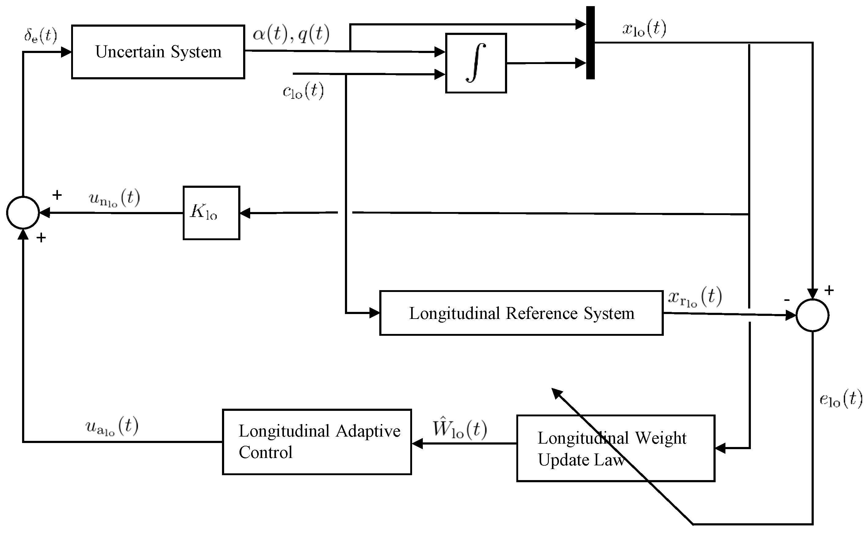
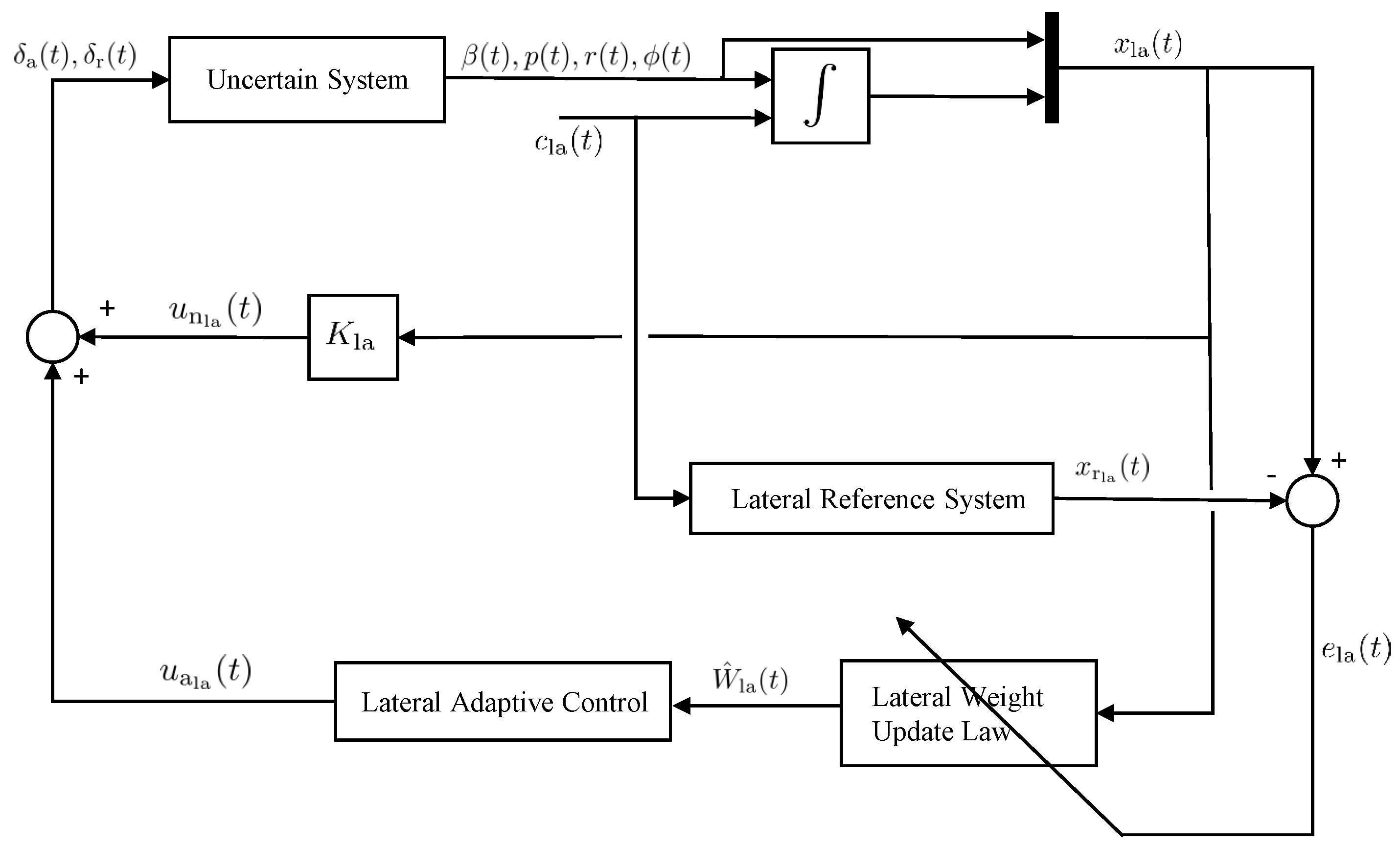
5.1.1. Longitudinal Control Design

For the decoupled longitudinal dynamics, we consider the state vector defined as $x_{{\mathrm{p}}_{\mathrm{lo}}}\left(t\right)={[\alpha \left(t\right),q\left(t\right)]}^{\mathrm{T}}$, with the respective system matrices:

$$A_{{\mathrm{p}}_{\mathrm{lo}}}=\left[\begin{array}{cc}-2.39\times {10}^{-1}& 1\\ 4.26& -1.19\times {10}^{-1}\end{array}\right],$$

(60)

$$B_{{\mathrm{P}}_{\mathrm{o}}}=\left[\begin{array}{c}-1.33\times {10}^{-4}\\ -1.84\times {10}^{-1}\end{array}\right].$$

(61)

LQR theory is used to design the nominal controller with $E_{{\mathrm{p}}_{\mathrm{lo}}}=[1,0]$ such that a desired angle of attack command is followed. The controller gain matrix $K_{\mathrm{lo}}$ is obtained using the highlighted augmented formulation (Equations (5) and (6)), along with the weighting matrices $Q_{\mathrm{lo}}=\mathrm{diag}[20000,25000,400000]$ to penalize $x_{\mathrm{lo}}\left(t\right)$ and $R_{\mathrm{lo}}=12.5$ to penalize $u_{\mathrm{lo}}\left(t\right)$, resulting in the following gain matrix:

$$\begin{array}{ccc}\hfill K_{\mathrm{lo}}& =& \left[\begin{array}{ccc}-1.65\times {10}^2& -6.09\times {10}^1& -1.79\times {10}^2\end{array}\right].\hfill \end{array}$$

(62)

The solution to $A_{{\mathrm{r}}_{\mathrm{lo}}}^{\mathrm{T}}{P}_{\mathrm{lo}}+P_{\mathrm{lo}}{A}_{{\mathrm{r}}_{\mathrm{lo}}}+R_{1_{\mathrm{lo}}}=0$, where $A_{{\mathrm{r}}_{\mathrm{lo}}}\triangleq A_{\mathrm{lo}}-B_{\mathrm{lo}}{K}_{\mathrm{lo}}$, is calculated using $R_{1_{\mathrm{lo}}}=\mathrm{diag}[1,1,100]$ for both the standard adaptive control design and the proposed controller. For the proposed design, we use Equations (25), (41) and (42) and resort to Equation (44) for enforcing ${∥e_{\mathrm{lo}}\left(t\right)∥}_{P_{\mathrm{lo}}}\le 0.5$. Additionally, note that ${\xi }_{\min }=10$ is selected to satisfy Equation (43), and we choose $a=2$. To visualize the overall longitudinal control design, a block diagram is provided in Figure 2.

5.1.2. Lateral Control Design

The decoupled lateral dynamics follows similarly. Specifically, we consider the state vector defined as $x_{{\mathrm{p}}_{\mathrm{la}}}\left(t\right)={[\beta \left(t\right),p\left(t\right),r\left(t\right),\varphi \left(t\right)]}^{\mathrm{T}}$, with the respective system matrices:

$$A_{{\mathrm{p}}_{\mathrm{la}}}=\left[\begin{array}{cccc}-6.97\times {10}^{-2}& -1.04\times {10}^{-2}& -9.99\times {10}^{-1}& -5.35\times {10}^{-3}\\ -1.31\times {10}^3& -2.03& -7.54\times {10}^{-3}& 0\\ 2.07& -1.55\times {10}^{-3}& -5.31\times {10}^{-2}& 0\\ -2.38\times {10}^{-4}& 8.54\times {10}^{-1}& -8.84\times {10}^{-3}& -3.00\times {10}^{-6}\end{array}\right],$$

(63)

$$B_{{\mathrm{p}}_{\mathrm{la}}}=\left[\begin{array}{cc}-2.47\times {10}^{-5}& -2.18\times {10}^{-4}\\ -8.04& 10.3\\ 3.17\times {10}^{-2}& 2.85\times {10}^{-1}\\ 0& 0\end{array}\right].$$

(64)

LQR theory is used to design the nominal controller with:

$$\begin{array}{ccc}\hfill E_{{\mathrm{p}}_{\mathrm{la}}}& =& \left[\begin{array}{cccc}1& 0& 0& 0\\ 0& 0& 0& 1\end{array}\right]\hfill \end{array}$$

(65)

such that a desired sideslip angle command and roll angle command are followed. The controller gain matrix $K_{\mathrm{la}}$ is obtained using the highlighted augmented formulation along with the weighting matrices $Q_{\mathrm{la}}=\mathrm{diag}[100,100,100,100,400000,2500]$ to penalize $x_{\mathrm{la}}\left(t\right)$ and $R_{\mathrm{la}}=\mathrm{diag}[1.25,50]$ to penalize $u_{\mathrm{la}}\left(t\right)$, resulting in the following gain matrix:

$$\begin{array}{ccc}\hfill K_{\mathrm{la}}& =& \left[\begin{array}{cccccc}2.78\times {10}^2& -9.08& -3.62\times {10}^1& -3.15\times {10}^1& 1.21\times {10}^2& -4.37\times {10}^1\\ 8.70\times {10}^1& 1.52\times {10}^{-1}& -2.72\times {10}^1& 1.30& 8.74\times {10}^1& 1.51\end{array}\right].\hfill \end{array}$$

(66)

The solution to $A_{{\mathrm{r}}_{\mathrm{la}}}^{\mathrm{T}}{P}_{\mathrm{la}}+P_{\mathrm{la}}{A}_{{\mathrm{r}}_{\mathrm{la}}}+R_{1_{\mathrm{la}}}=0$, where $A_{{\mathrm{r}}_{\mathrm{la}}}\triangleq A_{\mathrm{la}}-B_{\mathrm{la}}{K}_{\mathrm{la}}$ is calculated using $R_{1_{\mathrm{la}}}=\mathrm{diag}[1,1,1,1,100,100]$ for both the standard adaptive control design and the proposed controller. For the proposed design, we use Equations (25), (41) and (42) and resort to Equation (44) for enforcing ${∥e_{\mathrm{la}}\left(t\right)∥}_{P_{\mathrm{la}}}\le 0.5$. Additionally, note that ${\xi }_{\min }=10$ is selected to satisfy Equation (43), and we choose $a=2$. Similar to the previous section, a block diagram is provided in Figure 3 to visualize the control design using the decoupled lateral dynamics to control the overall uncertain system.

5.1.3. Nominal System without Uncertainty

The longitudinal and lateral controllers are augmented and applied to the overall coupled system. We first consider the case when there is no uncertainty in the system to show the nominal performance of the control designs. Figure 4 shows the response of the nominal control performance. It can also be seen from this figure that the error signals are not equal to zero, which is expected due to the coupling effects.

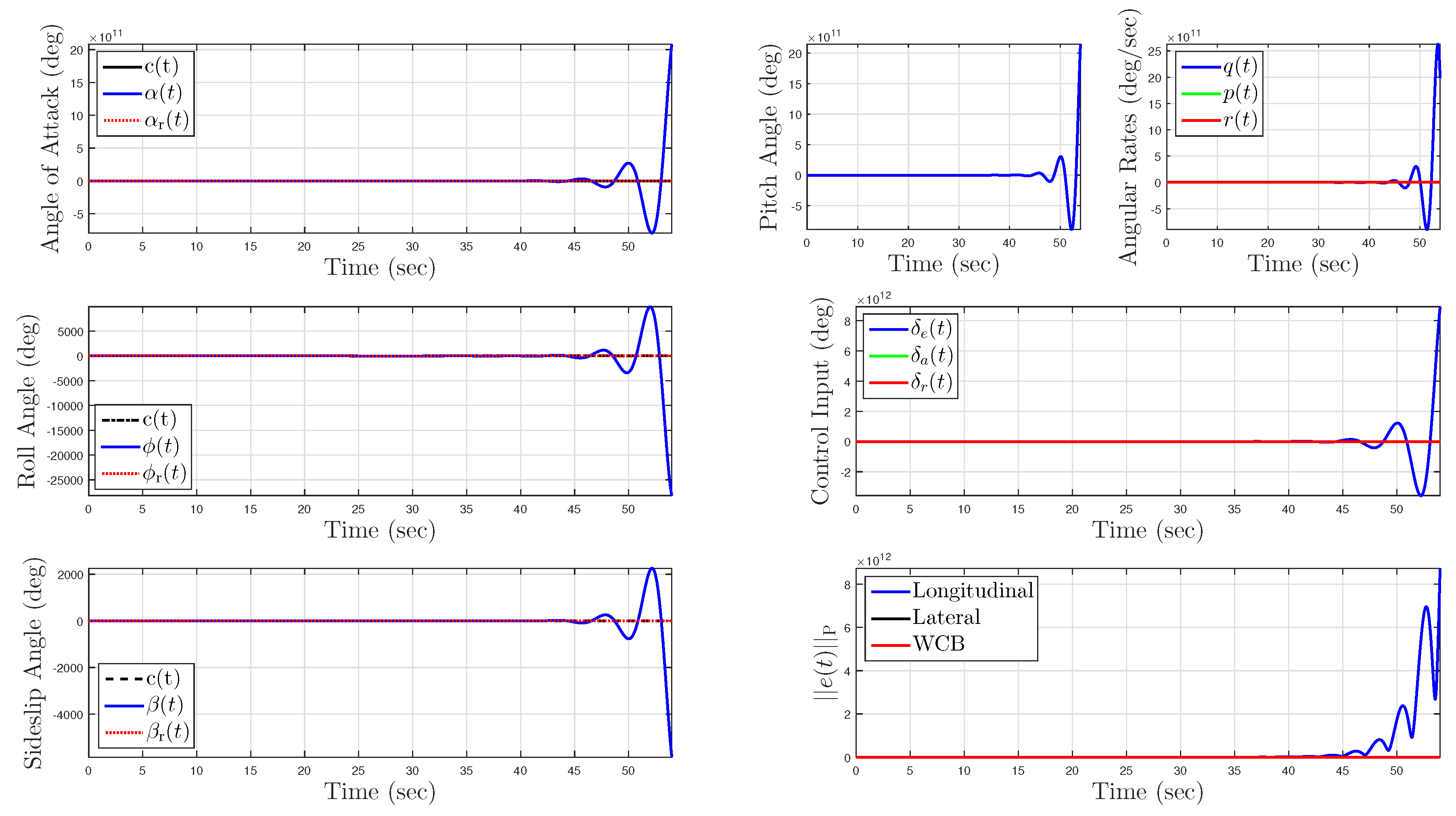
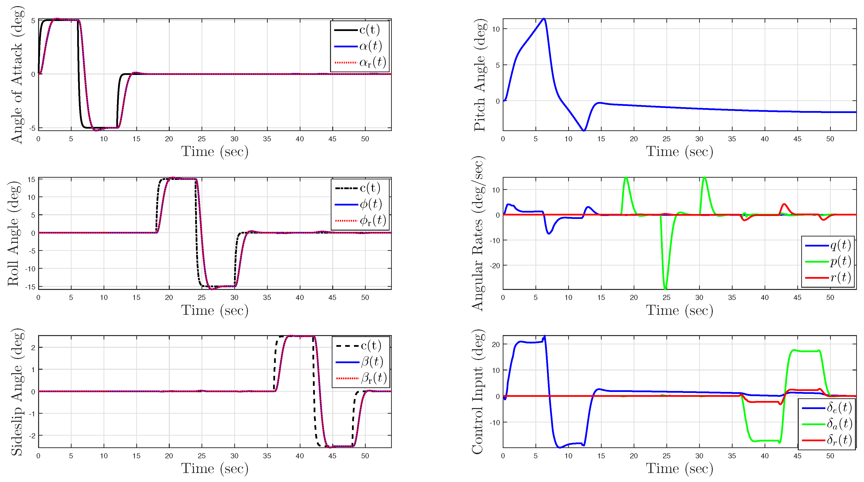
5.1.4. Uncertainty in Control Effectiveness and Stability Derivatives

We now consider the case when the control effectiveness matrix is unknown, as well as the stability derivatives $C_{m_{\alpha }}$ and $C_{n_{\beta }}$. For this purpose, we let $\Lambda =0.5I$, and we increase $C_{m_{\alpha }}$ and decrease $C_{n_{\beta }}$. Figure 5 shows the response with the nominal control, which goes unstable.

A standard adaptive control design is first implemented. For the standard adaptive controllers, we select the basis functions ${\sigma }_{\mathrm{lo}}\left(x_{\mathrm{lo}}\left(t\right)\right)={[x_{\mathrm{lo}}^{\mathrm{T}}\left(t\right)K_{\mathrm{lo}}^{\mathrm{T}},\alpha \left(t\right)]}^{\mathrm{T}}$ and ${\sigma }_{\mathrm{la}}\left(x_{\mathrm{la}}\left(t\right)\right)={[x_{\mathrm{la}}^{\mathrm{T}}\left(t\right)K_{\mathrm{la}}^{\mathrm{T}},\beta \left(t\right)]}^{\mathrm{T}}$ respectively for the longitudinal and lateral controllers. Figure 6 and Figure 7 show the standard adaptive control response. Specifically, Figure 6 shows that for a low learning gain, the system transient performance in the sideslip angle and angle of attack is poor. In addition, the control surface deflection angles exceed practical working limits. To improve the performance, the learning gain is increased as shown in Figure 7. Both the tracking performance and the control response improve; however, as seen in the bottom part of the figure, the standard adaptive controller is unable to enforce a pre-defined bound on the error.

To improve performance further and enforce a user-defined bound on the error, the proposed adaptive controller is then implemented using the same basis functions as the standard adaptive control design. Figure 8 and Figure 9 show the proposed controller performance using the gain varying control. Specifically, Figure 8 illustrates the superior tracking performance, and Figure 9 shows the guaranteed bound ${∥e\left(t\right)∥}_P\le 0.5$ for both the longitudinal and lateral dynamics.

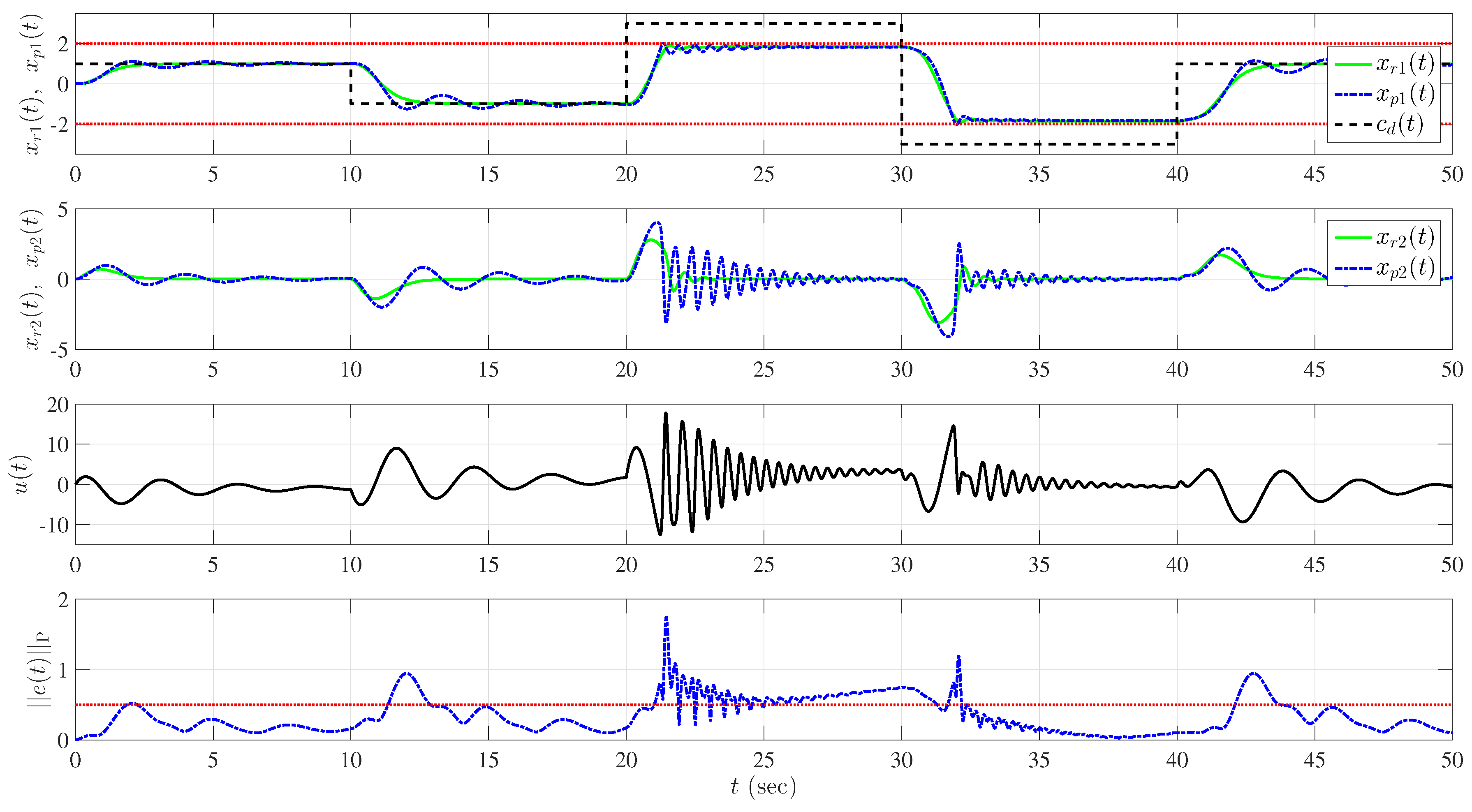
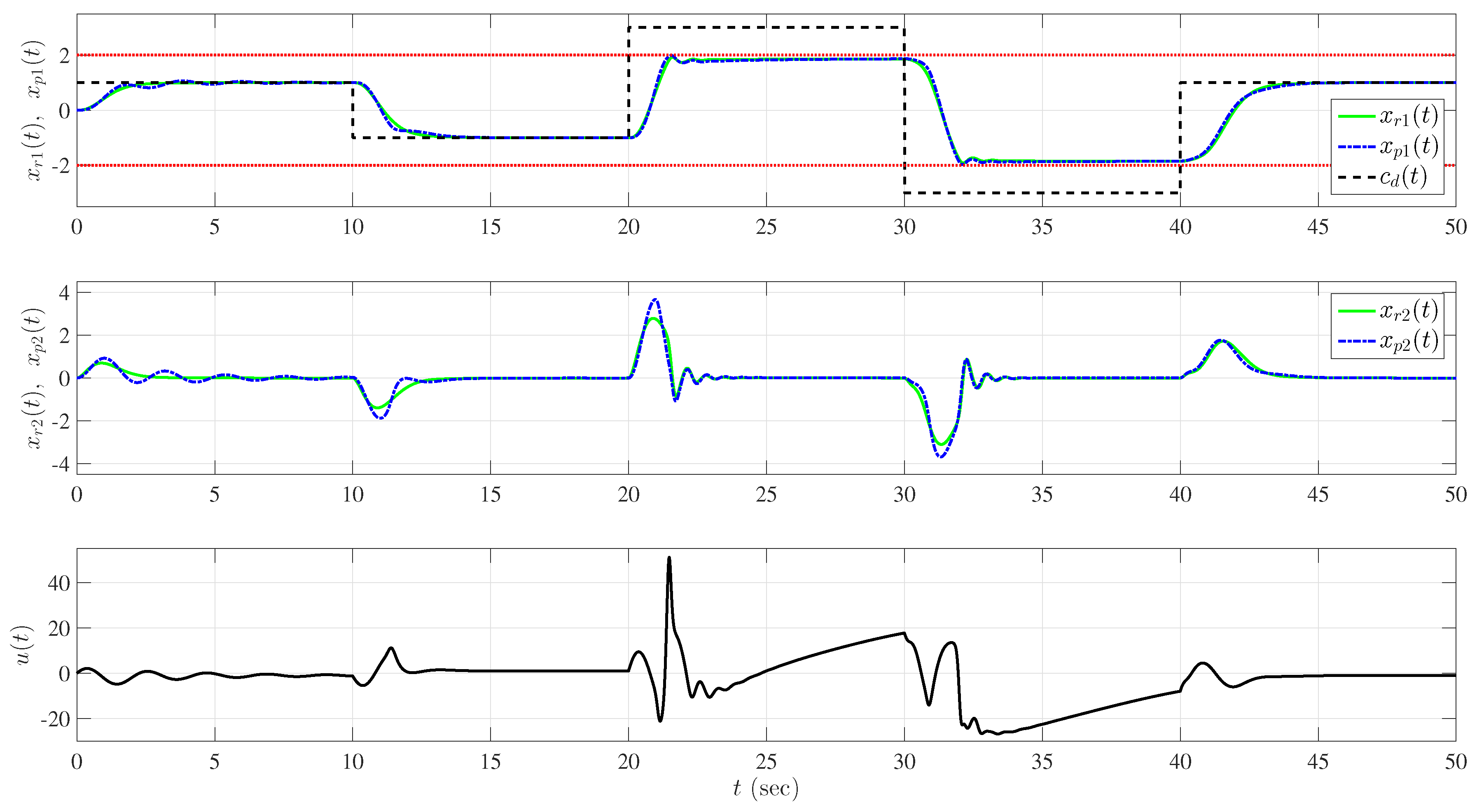
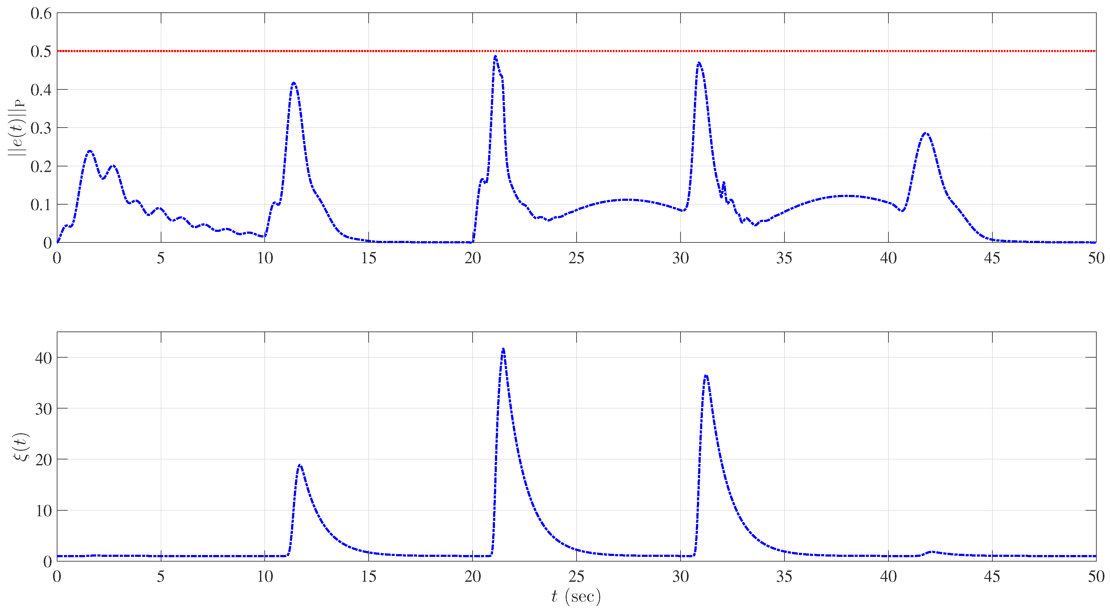
5.2. Example 2: Wing Rock Dynamics with Nonlinear Reference Model

We now consider the nonlinear dynamical system representing a controlled wing rock dynamics model given by:

$$\begin{array}{ccc}\hfill \left[\begin{array}{c}{\dot{x}}_{\mathrm{p}1}\left(t\right)\\ {\dot{x}}_{\mathrm{p}2}\left(t\right)\end{array}\right]& =& \left[\begin{array}{cc}0& 1\\ 0& 0\end{array}\right]\left[\begin{array}{c}{x}_{\mathrm{p}1}\left(t\right)\\ x_{\mathrm{p}2}\left(t\right)\end{array}\right]+\left[\begin{array}{c}0\\ 1\end{array}\right](\Lambda u\left(t\right)+{\delta }_{\mathrm{p}}\left(x_{\mathrm{p}}\left(t\right)\right)),\left[\begin{array}{c}{x}_{\mathrm{p}1}\left(0\right)\\ x_{\mathrm{p}2}\left(0\right)\end{array}\right]=\left[\begin{array}{c}0\\ 0\end{array}\right],\hfill \end{array}$$

(67)

where $x_{\mathrm{p}1}$ represents the roll angle in radians and $x_{\mathrm{p}2}$ represents the roll rate in radians per second. In Equation (67), ${\delta }_{\mathrm{p}}\left(x_{\mathrm{p}}\right)$ represents an uncertainty of the form ${\delta }_{\mathrm{p}}\left(x_{\mathrm{p}}\right)={\alpha }_1{x}_{\mathrm{p}1}+{\alpha }_2{x}_{\mathrm{p}2}+{\alpha }_3|x_{\mathrm{p}1}|x_{\mathrm{p}2}+{\alpha }_4\left|x_{\mathrm{p}2}\right|x_{\mathrm{p}2}+{\alpha }_5{x}_{\mathrm{p}1}^3,$ where ${\alpha }_i$, $i=1,\dots ,5$, are unknown parameters that are derived from the aircraft aerodynamic coefficients. For this numerical example, we set ${\alpha }_1=0.5$, ${\alpha }_2=1.0$, ${\alpha }_3=-1.0$, ${\alpha }_4=1.0$, ${\alpha }_5=0.5$ and $\Lambda =0.5$.

Note that for this example, the wing rock dynamics are linear, such that $f_{\mathrm{p}}\left(x_{\mathrm{p}}\left(t\right)\right)$ in Equation (45) is written as $A_{\mathrm{p}}{x}_{\mathrm{p}}\left(t\right)$. As a result, we let $E_{\mathrm{p}}=[1,0]$ such that the roll angle command is followed and use LQR theory with the augmented formulation Equations ((5) and (6)), along with the weighting matrices $Q=\mathrm{diag}[50,1,100]$ and $R=1$ to obtain the gain matrix $K=[12.30,5.06,10.0].$ In addition, we adopt the same nominal control structure to limit pilot authority as in [13] to design the nonlinear reference model as:

$$\begin{array}{ccc}\hfill {\dot{x}}_{\mathrm{r}}\left(t\right)& =& \left[\begin{array}{ccc}0& 1& 0\\ 0& 0& 0\\ 1& 0& 0\end{array}\right]x_{\mathrm{r}}\left(t\right)-\left[\begin{array}{c}0\\ 1\\ 0\end{array}\right]k\left(x_{\mathrm{r}}\left(t\right)\right)+\left[\begin{array}{c}0\\ 0\\ -1\end{array}\right]c\left(t\right),x_{\mathrm{r}}\left(t\right)=0,\hfill \end{array}$$

(68)

with $k\left(x_{\mathrm{r}}\left(t\right)\right)=K[x_{\mathrm{r}1}\left(t\right),x_{\mathrm{r}2}\left(t\right),\mathsf{\Phi }\left(x_{\mathrm{r}}\left(t\right)\right)x_{\mathrm{r}3}\left(t\right){]}^{\mathrm{T}}$, $c\left(t\right)=c_{\mathrm{d}}\left(t\right)\mathsf{\Phi }\left(x_{\mathrm{r}}\left(t\right)\right)$ and:

$$\begin{array}{ccc}\hfill \mathsf{\Phi }\left(x_{\mathrm{r}}\left(t\right)\right)& =& \tanh \left(5\right||x_{\mathrm{r}1}\left(t\right)|-2|).\hfill \end{array}$$

(69)

Note that $c_{\mathrm{d}}\left(t\right)$ is a desired command applied by the pilot and $\mathsf{\Phi }\left(x_{\mathrm{r}}\left(t\right)\right)$ is a nonlinear function that limits the pilot authority by constraining the absolute value of the roll angle to remain less than or equal to two. Motivated from the structure of the nonlinear reference model, the feedback linearization term is designed as:

$$\begin{array}{c}\hfill v(·)=-Ke\left(t\right)+K[x_1\left(t\right),x_2\left(t\right),\mathsf{\Phi }\left(x\left(t\right)\right)x_3\left(t\right){]}^{\mathrm{T}}-K[x_{\mathrm{r}1}\left(t\right),x_{\mathrm{r}2}\left(t\right),\mathsf{\Phi }\left(x_{\mathrm{r}}\left(t\right)\right)x_{\mathrm{r}3}\left(t\right){]}^{\mathrm{T}},\end{array}$$

(70)

such that Equation (53) holds. Using this, we select the basis function as:

$$\begin{array}{c}\hfill \sigma (·)=[x_{\mathrm{p}1},x_{\mathrm{p}2},|x_{\mathrm{p}1}|x_{\mathrm{p}2},\left|x_{\mathrm{p}2}\right|x_{\mathrm{p}2},x_{\mathrm{p}1}^3,x^{\mathrm{T}}\left(t\right)K^{\mathrm{T}},v^{\mathrm{T}}(·){]}^{\mathrm{T}},\end{array}$$

(71)

and we set $R=I_{3\times 3}$ for both the standard adaptive controller and the proposed adaptive controller. Furthermore, for the proposed design, we use Equations (55), (41) and (56) and resort to Equation (44) for enforcing ${∥e\left(t\right)∥}_P\le 0.5$. Additionally, note that ${\xi }_{\min }=1$ is selected to satisfy Equation (43), and we choose $a=2$.

Figure 10 shows the standard adaptive control response. It can be seen from the figure that even though the roll angle command is reasonably followed, the roll rate and the control response have undesirable high-frequency content, which can cause instability. In addition, as seen in the bottom part of the figure, the standard adaptive controller is unable to enforce a pre-defined bound on the error.

To improve performance and enforce a user-defined bound on the error, the proposed adaptive controller is then implemented. Figure 11 and Figure 12 show the proposed controller performance using the gain varying control. It is clear from Figure 11 that the proposed adaptive controller obtains superior command-following performance, and Figure 12 shows that the system error stays in the a priori given, user-defined performance bound.

6. Conclusions

We proposed a direct uncertainty minimization approach that uses modification terms in the adaptive control law and the update law to suppress the effect of system uncertainty on the transient system response through a gradient minimization procedure for improved system performance. In addition, the use of a varying gain on the modification term was shown to keep the system error approximately within a priori given, user-defined error performance bounds. The proposed approach was then generalized to incorporate a nonlinear reference model to better capture the desired closed-loop system performance for a class of nonlinear uncertain dynamical systems. Two illustrative numerical examples were included to demonstrate the efficacy of the proposed adaptive control framework. Future research will include generalizations of the proposed framework to output feedback adaptive control, as well as applications to large-scale dynamical systems.

References

1. Duarte, M.A.; Narendra, K.S. Combined direct and indirect approach to adaptive control. IEEE Trans. Autom. Control 1989, 34, 1071–1075. [Google Scholar] [CrossRef]
2. Slotine, J.J.E.; Li, W. Composite adaptive control of robot manipulators. Automatica 1989, 25, 509–519. [Google Scholar] [CrossRef]
3. Lavretsky, E. Combined/composite model reference adaptive control. IEEE Trans. Autom. Control 2009, 54, 2692. [Google Scholar] [CrossRef]
4. Volyanskyy, K.Y.; Calise, A.J.; Yang, B.J. A novel Q-modification term for adaptive control. In Proceedings of the American Control Conference, Minneapolis, MN, USA, 14–16 June 2006.
5. Volyanskyy, K.Y.; Calise, A.J.; Yang, B.J.; Lavretsky, E. An error minimization method in adaptive control. In Proceedings of the AIAA Guidance, Navigation, and Control Conference, Keystone, CO, USA, 21–24 August 2006.
6. Volyanskyy, K.Y.; Haddad, M.; Calise, A.J. A new neuroadaptive control architecture for nonlinear uncertain dynamical systems: Beyond-and-modifications. IEEE Trans. Neural Netw. 2009, 20, 1707–1723. [Google Scholar] [CrossRef] [PubMed]
7. Chowdhary, G.; Johnson, E.N. Theory and flight-test validation of a concurrent-learning adaptive controller. J. Guid. Control Dyn. 2011, 34, 592–607. [Google Scholar] [CrossRef]
8. Chowdhary, G.; Yucelen, T.; Mühlegg, M.; Johnson, E.N. Concurrent learning adaptive control of linear systems with exponentially convergent bounds. Int. J. Adapt. Control Signal Process. 2013, 27, 280–301. [Google Scholar] [CrossRef]
9. Yucelen, T.; Johnson, E.N. Artificial basis functions in adaptive control for transient performance improvement. In Proceedings of the AIAA Guidance, Navigation, and Control Conference, Boston, MA, USA, 19–22 August 2013.
10. Gruenwald, B.; Yucelen, T.; Fravolini, M. Performance oriented adaptive architectures with guaranteed bounds. In Proceedings of the AIAA Infotech@Aerospace Conference, Kissimmee, FL, USA, 5–9 January 2015.
11. Gruenwald, B.; Yucelen, T. On transient performance improvement of adaptive control architectures. Int. J. Control 2015, 88, 2305–2315. [Google Scholar] [CrossRef]
12. Yucelen, T.; Gruenwald, B.; Muse, J.; De La Torre, G. Adaptive control with nonlinear reference systems. In Proceedings of the American Control Conference, Chicago, IL, USA, 1–3 July 2015.
13. Arabi, E.; Gruenwald, B.C.; Yucelen, T.; Nguyen, N.T. A set-theoretic model reference adaptive control architecture for disturbance rejection and uncertainty suppression with strict performance guarantees. Int. J. Control 2017, in press. [Google Scholar]
14. Narendra, K.S.; Annaswamy, A.M. Stable Adaptive Systems; Courier Corporation: Mineola, NY, USA, 2012. [Google Scholar]
15. Lavretsky, E.; Wise, K.A. Robust Adaptive Control; Springer: New York, NY, USA, 2013. [Google Scholar]
16. Ioannou, P.A.; Sun, J. Robust Adaptive Control; Courier Corporation: Mineola, NY, USA, 2012. [Google Scholar]
17. Khalil, H.K. Nonlinear Systems; Prentice Hall: Upper Saddle River, NJ, USA, 1996. [Google Scholar]
18. Lewis, F.L.; Liu, K.; Yesildirek, A. Neural net robot controller with guaranteed tracking performance. IEEE Trans. Neural Netw. 1995, 6, 703–715. [Google Scholar] [CrossRef] [PubMed]
19. Lewis, F.L.; Yesildirek, A.; Liu, K. Multilayer neural-net robot controller with guaranteed tracking performance. IEEE Trans. Neural Netw. 1996, 7, 388–399. [Google Scholar] [CrossRef] [PubMed]
20. Pomet, J.B.; Praly, L. Adaptive nonlinear regulation: Estimation from the Lyapunov equation. IEEE Trans. Autom. Control 1992, 37, 729–740. [Google Scholar] [CrossRef]
21. Krstic, M.; Kanellakopoulos, I.; Kokotovic, P.V. Nonlinear and Adaptive Control Design; Wiley: New York, NY, USA, 1995. [Google Scholar]
22. Haddad, W.M.; Chellaboina, V. Nonlinear Dynamical Systems and Control: A Lyapunov-Based Approach; Princeton University Press: Princeton, NJ, USA, 2008. [Google Scholar]
Figure 1. A candidate f ( e ) for Equation (44).
Machines 05 00009 g001
Figure 2. Block diagram of separated longitudinal control design.
Machines 05 00009 g002
Figure 3. Block diagram of separated lateral control design.
Machines 05 00009 g003
Figure 4. Nominal controller performance without uncertainty.
Machines 05 00009 g004
Figure 5. Nominal controller performance with uncertainty in Λ, C m α and C n β .
Machines 05 00009 g005
Figure 6. Standard adaptive controller performance with uncertainty in Λ, C m α and C n β ( Γ lo = I 2 × 2 and Γ la = I 3 × 3 ).
Machines 05 00009 g006
Figure 7. Standard adaptive controller performance with uncertainty in Λ, C m α and C n β ( Γ lo = 100 I 2 × 2 and Γ la = 100 I 3 × 3 ).
Machines 05 00009 g007
Figure 8. Proposed gain varying adaptive control performance with uncertainty in Λ, C m α and C n β ( Γ lo = I 2 × 2 and Γ la = diag [ 0.1 , 1 , 1 ] , ξ 0 = 10 and a = 2 ).
Machines 05 00009 g008
Figure 9. System error bounds and adaptation gain for Figure 8.
Machines 05 00009 g009
Figure 10. Standard adaptive controller performance ( γ = 1 ).
Machines 05 00009 g010
Figure 11. Proposed gain varying adaptive control performance ( γ = 1 and γ ξ = 1 , ξ 0 = 1 and a = 2 ).
Machines 05 00009 g011
Figure 12. System error bounds and adaptation gain for Figure 11.
Machines 05 00009 g012