Integrated Condition Monitoring and Prognosis Method for Incipient Defect Detection and Remaining Life Prediction of Low Speed Slew Bearings

Abstract

This paper presents an application of multivariate state estimation technique (MSET), sequential probability ratio test (SPRT) and kernel regression for low speed slew bearing condition monitoring and prognosis. The method is applied in two steps. Step (1) is the detection of the incipient slew bearing defect. In this step, combined MSET and SPRT is used with circular-domain kurtosis, time-domain kurtosis, wavelet decomposition (WD) kurtosis, empirical mode decomposition (EMD) kurtosis and the largest Lyapunov exponent (LLE) feature. Step (2) is the prediction of the selected features’ trends and the estimation of the remaining useful life (RUL) of the slew bearing. In this step, kernel regression is used with time-domain kurtosis, WD kurtosis and the LLE feature. The application of the method is demonstrated with laboratory slew bearing acceleration data.

1. Introduction

Steelmaking industry has many critical processes which rely on low rotating slew bearings. These bearings are often used in harsh conditions and have high replacement cost with long delivery lead time. Therefore, it is important to monitor their condition at all times. Typical maintenance schedule is replace the bearings which have been in operation of set number of hours. However, due to their low speeds, the bearings run to failure without appropriate condition monitoring method. These can lead to a high level of risk and sub-utilization of the actual bearing useful life. To reduce the risk of sudden bearing failure and optimise the use of the bearing, integrated condition monitoring and prognosis method for low speed slew bearings is needed.

In order to monitor the condition of slew bearings, a method that able to extract the trends related to degradation condition is necessary. Henao et al. [1] presents a review of diagnostic techniques for electrical machines. The summary of recently proposed methods for performing diagnostics in nonstationary conditions were categorised into four: (1) Frequency domain approach using the rotational invariance technique; (2) Time domain analysis-based DWT; (3) Slip-frequency approach based on the description of the instantaneous frequency of an extracted fault component against slip; (4) Diagnosis in the time-frequency domain using STFT, CWT, WVD, Choi-Willians distribution (CWD), and Zhao-Atlas-Marks distribution. Currently, artificial intteligent (AI) techniques remain a priority tool to support the condition monitoring and fault diagnosis methods especially in the decision process [1,2]. These techniques have been widely developed in recent years, even though they are not yet applied in the industrial practice [1].

A condition monitoring method for slew bearings using kurtosis extracted from vibration and acoustic emission signals as condition parameters was proposed by Rodgers [3]. A recent slew bearing condition monitoring and fault diagnosis study [4] combined ensemble empirical mode decomposition (EEMD) and multiscale principal component analysis (MSPCA). The method successfully predicted defect frequency of artificially damaged inner race which matched with the ball pass frequency inner race (BPFI). However, the practical challenge is how to detect the incipient defect of slew bearing from low energy vibration of naturally induced defect and predict RUL based on the observation parameters. To date, prognosis methods have been mainly applied in typical rolling element bearings with rotational speed greater than 1000 rpm [5,6,7]. Lei et al. [8] proposed the application of particle filtering (PF) to estimate model parameters from real-time measured data. The model parameters were updated adaptively, which eventually were used to predict the remaining useful life (RUL) of machineries. The operation conditions of tested bearings are 1500, rpm 1650 rpm and 1800 rpm. Subsequently, Li et al. [9] highlighted the main shortcoming of traditional PF that is attributed to the subjective selection of the first predicting time (FPT), i.e., the triggered time to start the prediction process. The authors, thereafter, improved the methodology by means of adaptive FPT selection via stochastic approach. The bearing was naturally degraded during the experiment with rotational speed of 1800 rpm. The prognosis of low speed bearings with naturally induced defects has not been explored. Prognosis method has not been applied in the study of low rotational speed slew bearing [4,10,11]. This paper present both condition monitoring and prognosis method.

The method employs a multivariate state estimation technique (MSET) and a sequential probability ratio test (SPRT) to identify subtle changes in bearing condition, and kernel regression to predict the trend of the change and to estimate the RUL of the slew bearing. MSET was first introduced by Singer [12] and developed further by the Argonne National Laboratory [13,14]. Over the years, the technique has been applied successfully in many applications such as in the analysis of nuclear power reactor signals [12,13,14,15]. Recently, MSET has been used in prognosis and fault diagnosis studies e.g., the estimation of the remaining useful life of electronic products [16], the monitoring of lithium-ion battery performance [17] and early fault diagnosis of wind turbines [18]. The previous study used MSET to correlate the features of vibration signal acquired from low speed slew bearing [19].

SPRT was initially introduced by Wald [20,21] as a sequential statistical method. This method has been shown to work well either as a stand-alone decision-making method [22,23,24,25,26] or as an integrated method together with MSET [14,27]. When integrated with MSET, SPRT can be used to analyze the MSET result. SPRT can also be combined with auto-associative kernel regression algorithm [28]. Traditionally, kernel regression has been applied in image processing studies such as in image de-noising and enhancement [29] and image reconstruction [30]. It is an appropriate prediction method [31] and adopted in this paper.

This paper is organized as follows. Section 2 describes how features such as circular-domain kurtosis, time-domain kurtosis, WD kurtosis, EMD kurtosis and LLE feature are computed and monitored using MSET and SPRT to detect the incipient slew bearing defect and used in the kernel regression computation to predict the trends of these features. Section 3 describes the experimental set-up. Section 4 presents the results and discusses the proposed integrated condition monitoring and prognosis method including the estimation of the RUL. Finally, Section 5 presents the conclusions of the current work.

2. Integrated Condition Monitoring and Prognosis Method for Low Speed Slew Bearings

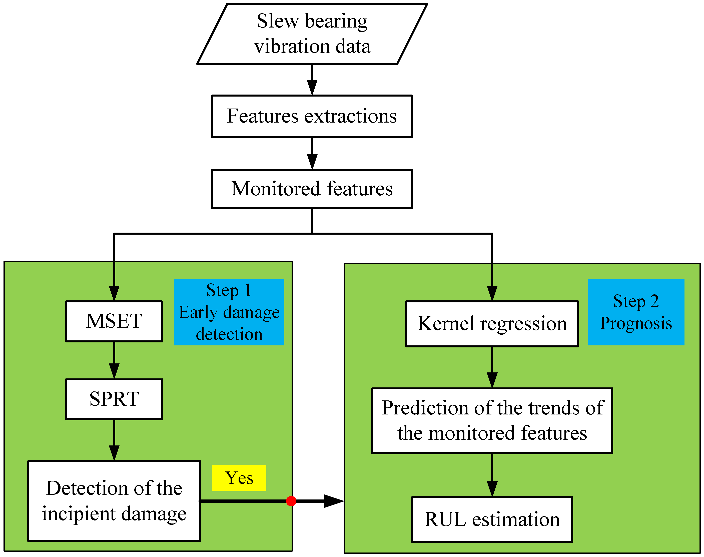
The proposed integrated condition-monitoring and prognosis method is implemented as follows: Step (1) is the detection of the incipient slew bearing defect where combined MSET and SPRT is used to process circular-domain kurtosis [32], time-domain kurtosis [32], WD kurtosis [32], EMD kurtosis [32] and LLE feature [33]. Step (2) predicts the trends of the selected features and estimates the RUL of the slew bearing. In this step, kernel regression is used to predict the trend of the time-domain kurtosis, WD kurtosis and the LLE features. Step (2) is initiated when the incipient bearing defect from Step (1) is registered. Figure 1 illustrates the computational implementation of the method.

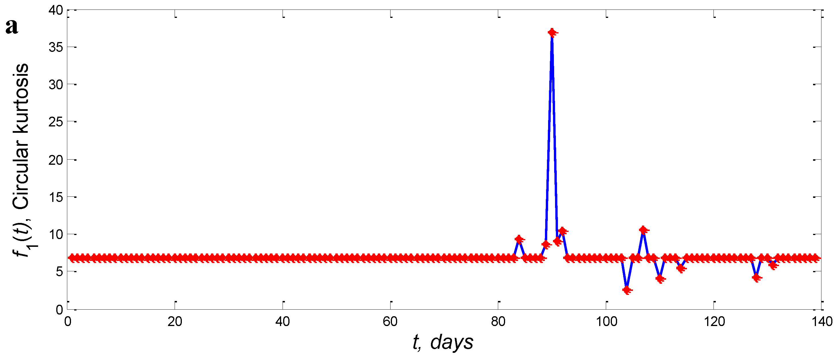
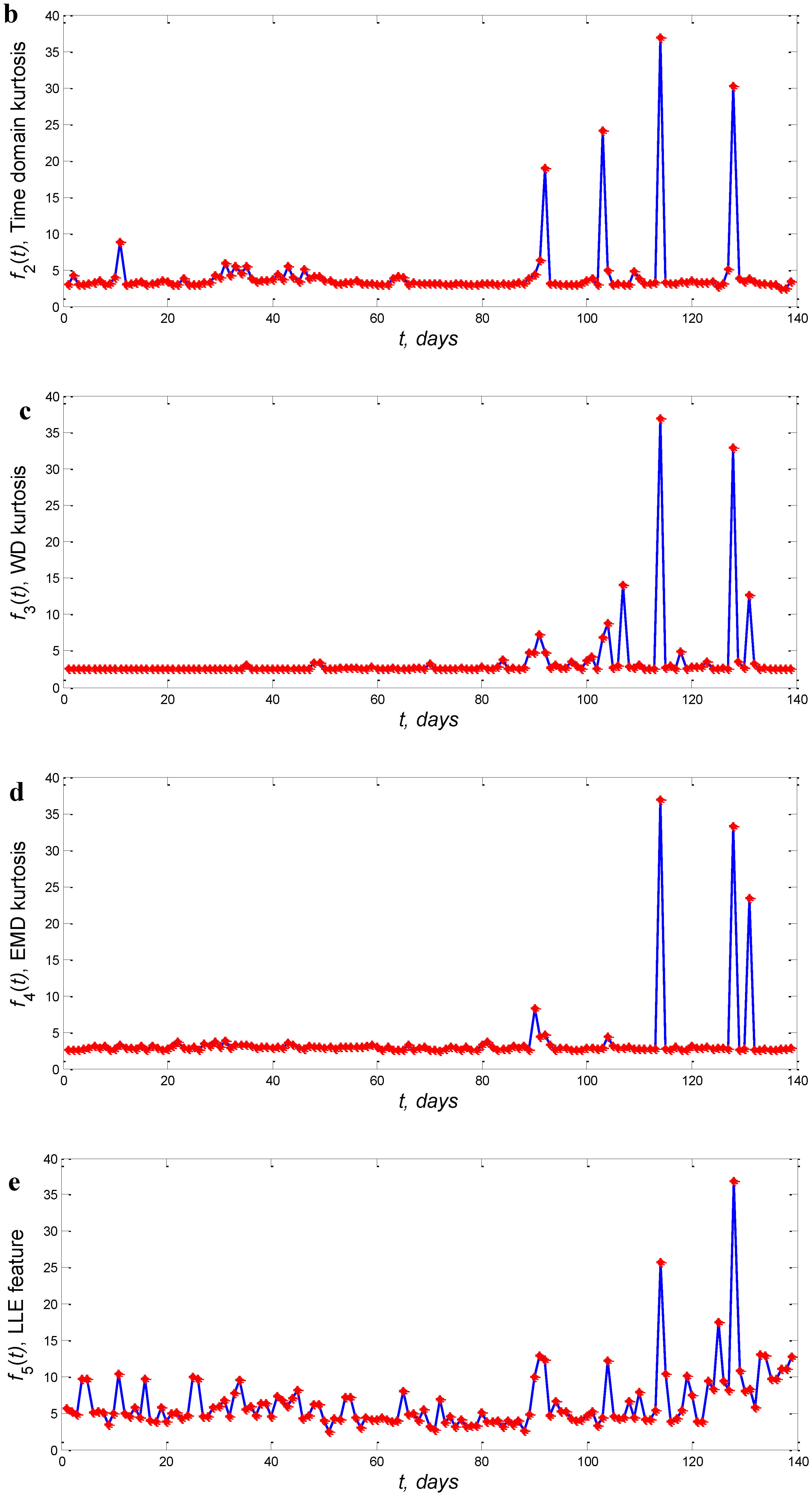
Examples of features extracted from slew bearing acceleration data are shown in Figure 2. How these features were extracted has been described in Refs. [32,33]. It is apparent that the features do not display any clear trend. In this paper, circular kurtosis, time-domain kurtosis, WD kurtosis and EMD kurtosis are employed to obtain the bearing degradation parameter for prognosis method.

2.1. Step (1) Detection of the Incipient Slew Bearing Defect Using MSET and SPRT

2.1.1. The Multivariate State Estimation Technique (MSET)

MSET is a technique that typically used to analyse anomalous process based on sensor reading and input parameters during the online condition monitoring. This technique has been applied in process monitoring, signal validation and surveillance applications [12,13,14,15,16,17,18,19,27]. The previous study used MSET to correlate the features of vibration signal acquired from low speed slew bearing such as largest Lyapunov exponent, approximate entropy, margin factor and impulse factor. In the present study, MSET is employed for different features i.e., circular-domain kurtosis, time-domain kurtosis, wavelet decomposition-kurtosis and empirical mode decomposition-kurtosis.

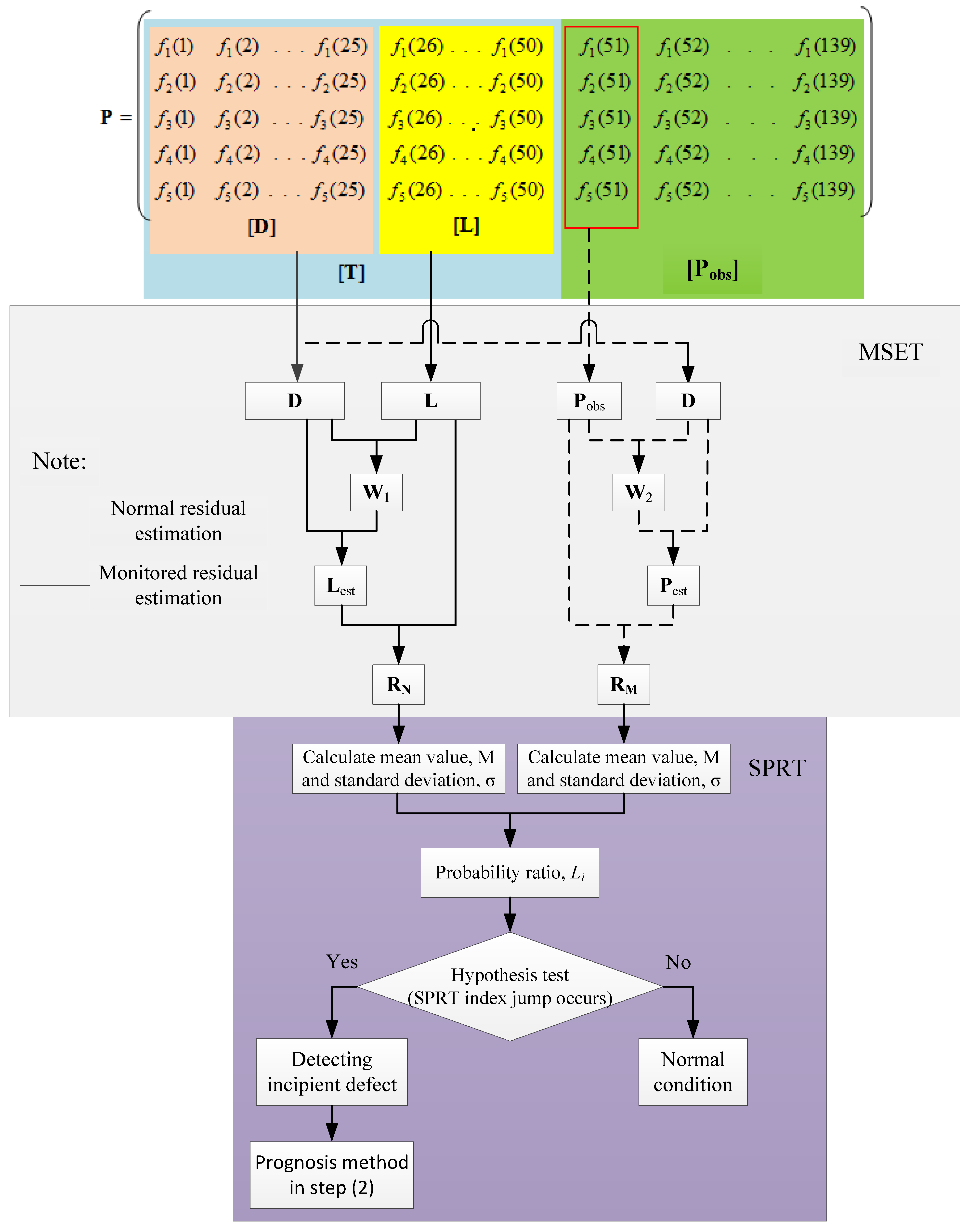
The MSET algorithm is applied systematically in 5 steps [16] as shown in Figure 3 in the first and second blocks. First, data matrix P is created where the row elements of P are the extracted features and the columns are the measurement time i.e., days. Data matrix P of size m features × n days is defined in Equation (1).

$$\begin{array}{ll}day1day2day3dayn& \\ P=\left[\begin{array}{ccccc}{f}_1(1)\hfill & f_1(2)\hfill & f_1(3)\hfill & \dots & f_1(n)\hfill \\ f_2(1)\hfill & f_2(2)\hfill & f_2(3)\hfill & \dots & f_2(n)\hfill \\ f_3(1)\hfill & f_3(2)\hfill & f_3(3)\hfill & \dots & f_3(n)\hfill \\ ⋮& ⋮& ⋮& \ddots & ⋮\\ f_m(1)\hfill & f_m(2)\hfill & f_m(3)\hfill & \dots & f_m(n)\hfill \end{array}\right]\hfill & \begin{array}{l}feature1\\ feature2\\ \\ \\ \\ featurem\end{array}\hfill \end{array}$$

(1)

Second, data matrix P is subdivided into two matrices: training matrix T and observation matrix P_obs. T is further divided into memory matrix D and remaining training matrix L. It should be noted that T holds data from the normal state while P_obs holds the monitored state, as shown in Equation (2).

$$P=\left[\begin{array}{ccccccccccc}{f}_1(1)\hfill & f_1(2)\hfill & \dots & f_1(n_D)\hfill & f_1(n_D+1)\hfill & \dots & f_1(n_L)\hfill & f_1(n_L+1)\hfill & f_1(n_L+2)\hfill & \dots & f_1(n)\hfill \\ f_2(1)\hfill & f_2(2)\hfill & \dots & f_2(n_D)\hfill & f_2(n_D+1)\hfill & \dots & f_2(n_L)\hfill & f_2(n_L+1)\hfill & f_2(n_L+2)\hfill & \dots & f_2(n)\hfill \\ f_3(1)\hfill & f_3(2)\hfill & \dots & f_3(n_D)\hfill & f_3(n_D+1)\hfill & \dots & f_3(n_L)\hfill & f_3(n_L+1)\hfill & f_3(n_L+2)\hfill & \dots & f_3(n)\hfill \\ ⋮& ⋮& & ⋮& ⋮& & ⋮& ⋮& ⋮& & ⋮\\ f_m(1)\hfill & f_m(2)\hfill & \dots & f_m(n_D)\hfill & f_m(n_D+1)\hfill & \dots & f_m(n_L)\hfill & f_m(n_L+1)\hfill & f_m(n_L+2)\hfill & \dots & f_m(n)\hfill \end{array}\right]$$

(2)

where n_D is the number of days in D matrix and n_L is the number of days in L matrix.

Third, the weight vector for the normal state (w₁) is calculated as follows [16]

$$w_1={(D^{\mathrm{T}}\otimes D)}^{-1}•(D^{\mathrm{T}}\otimes L)$$

(3)

and the weight vector for the observation state (w₂) is calculated as follows [16]

$$w_2={(D^{\mathrm{T}}\otimes D)}^{-1}•(D^{\mathrm{T}}\otimes P_{\mathrm{obs}})$$

(4)

Operator $\otimes$ is a non-linear operator. Several non-linear operators can be selected for MSET [34]. The most popular operator is the Euclidean distance, which is the one adopted in this paper.

Fourth, the normal estimate matrix (L_est) is computed by Equation (5)

$$L_{\mathrm{est}}=D•w_1$$

(5)

and the estimate matrix of monitored state (P_est) is calculated by Equation (6)

$$P_{\mathrm{est}}=D•w_2$$

(6)

Fifth, the normal residual matrix (R_N) is the difference between L_est and L and calculated by Equation (7).

$$R_{\mathrm{N}}=L_{\mathrm{est}}-L$$

(7)

And the residual matrix of monitored state (R_M) is the difference between P_est and P_obs and calculated by Equation (8).

$$R_{\mathrm{M}}=P_{\mathrm{est}}-P_{\mathrm{obs}}$$

(8)

2.1.2. The Sequential Probability Ratio Test (SPRT)

SPRT is a sequential statistical binary hypothesis technique [20,21] that has been used as a simple and effective stand-alone decision-making technique for engineering systems such as the surveillance of nuclear power plant components [23], statistical damage classification of an automotive system [24], long-term radiation monitoring [25], and multiple fault recognition in gearboxes [26]. SPRT has been integrated with MSET to analyse the output of the MSET and digitally assess the condition of the system being monitored [14,27]. With this capability SPRT is a potential early warning method embeddable in online monitoring systems.

To detect the incipient slew bearing defect, SPRT utilizes the outputs of MSET, the normal residual matrix (R_N) and the residual matrix of monitored state (R_M) as shown in Figure 3. The MSET outputs are then subjected to binary hypothesis test, where the objective is to assess whether the bearing is still in normal condition or already in defective condition. The decision making process is based on a set of hypotheses: normal condition denoted by a null hypothesis (H₀) and defect condition denoted by (H). In practice, there could be more than one hypothesis (H), i.e., H₁, H₂, …, H_z (see

Table 1. Hypotheses for SPRT.

Hypothesis	Statistical Properties
	Mean (M)	Standard Deviation (σ)
1. Normal condition (H0)	Mnormal (Table 5)	σnormal = 0.439 (Table 6)
2. Abnormal condition 1 (H1)	Mmonitored > Mmax	σ
3. Abnormal condition 2 (H2)	Mmonitored < Mmin	σ
4. Abnormal condition 3 (H3)	Mmin < Mmonitored < Mmax	σmonitored > σnormal
5. Abnormal condition 4 (H4)	Mmin < Mmonitored < Mmax	σmonitored < σnormal

Note: M_min < M_normal < M_max

). It should be noted that with more hypotheses used, the greater the accuracy of the decision making will be.

In SPRT analysis (see Figure 3), L_i the ratio of the probability of H₀ and the probability of H is calculated. The decision is then made based on the SPRT index calculated as follows [35]:

$${SPRT}_{index}=\ln (L_i)$$

(9)

where L_i is given by

$$L_i=\frac{\mathrm{probability}\mathrm{of}\mathrm{statistical}\mathrm{properties}\left\{S_i\right\}\mathrm{given}\mathrm{H}\mathrm{is}\mathrm{true}}{\mathrm{probability}\mathrm{of}\mathrm{statistical}\mathrm{properties}\left\{S_i\right\}\mathrm{given}{\mathrm{H}}_0\mathrm{is}\mathrm{true}}$$

(10)

where S_i are the statistical properties e.g., mean, M and standard deviation, σ of observation features at the monitored measurement day.

2.2. Step (2) Prediction of the Future State of Monitored Parameters Using Modified Kernel Regression

Kernel regression [36,37,38] is a non-parametric regression technique used to estimate regression function f(x, y) that best fit non-linear data set (X_j, Y_j). X_j in this paper refers to the measurement day and Y_j is the value of the extracted feature. Unlike linear regression or polynomial regression, kernel regression does not assume any underlying distribution to estimate the regression function [39]. The kernel regression uses a set of identical weighted function called local kernels to each observation data point. The kernel basis function depends only on the kernel width from local data point X to a set of neighboring locations x. The procedures of the proposed kernel regression-based prognostic are implemented in three systematic steps.

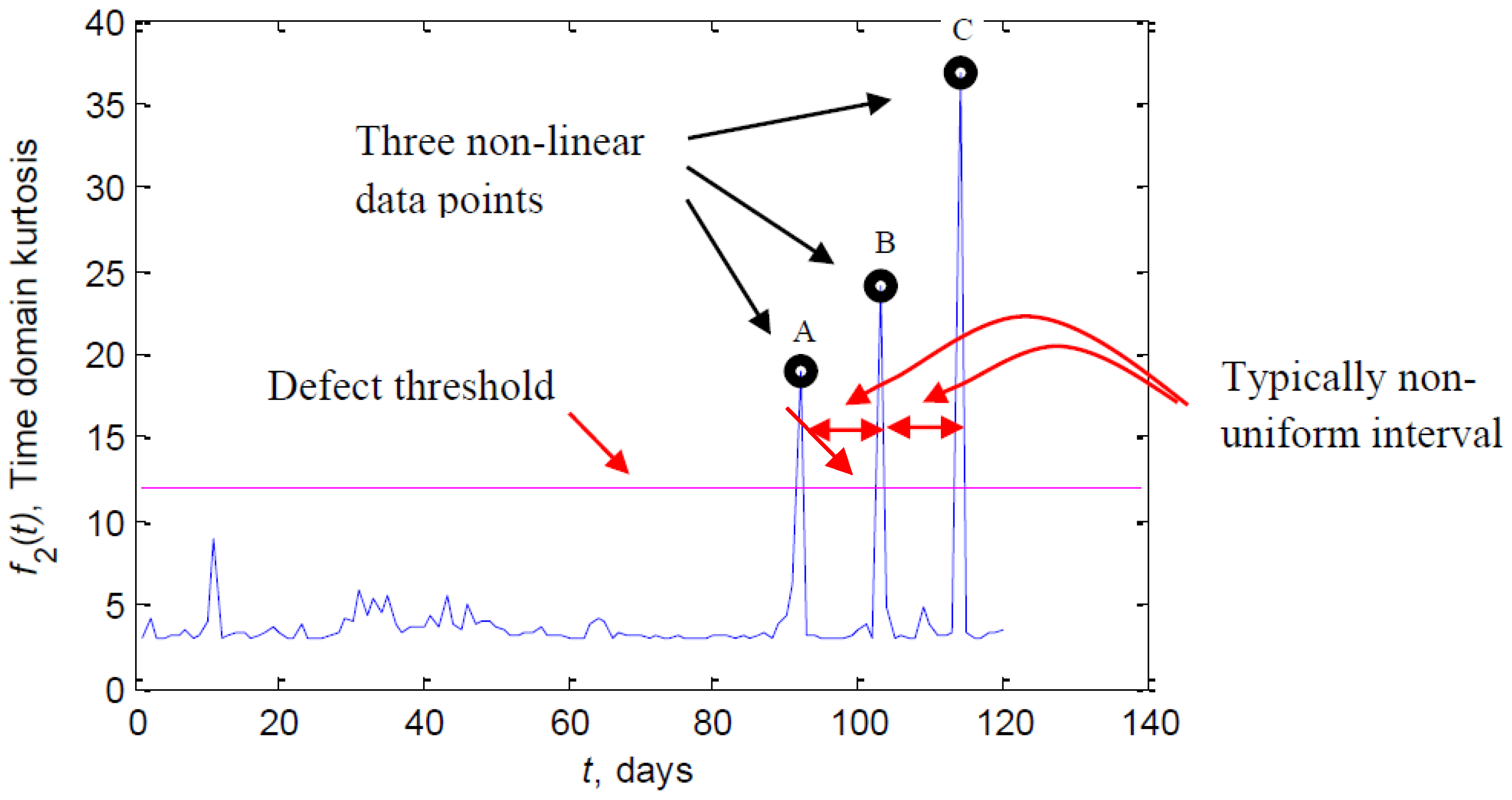
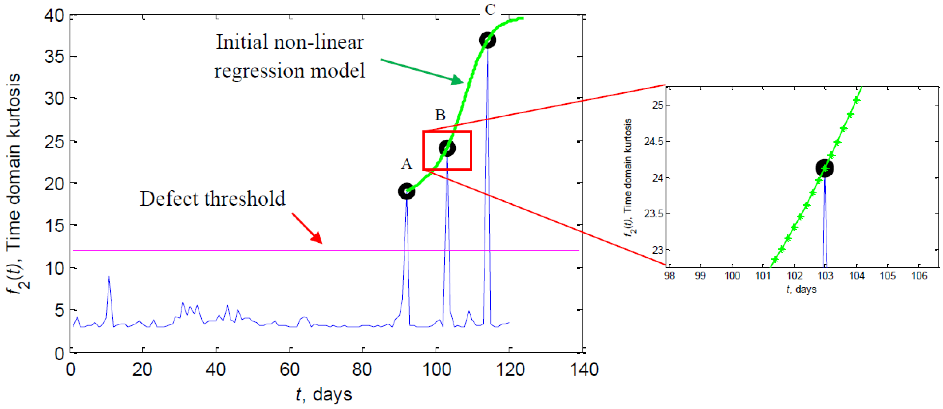
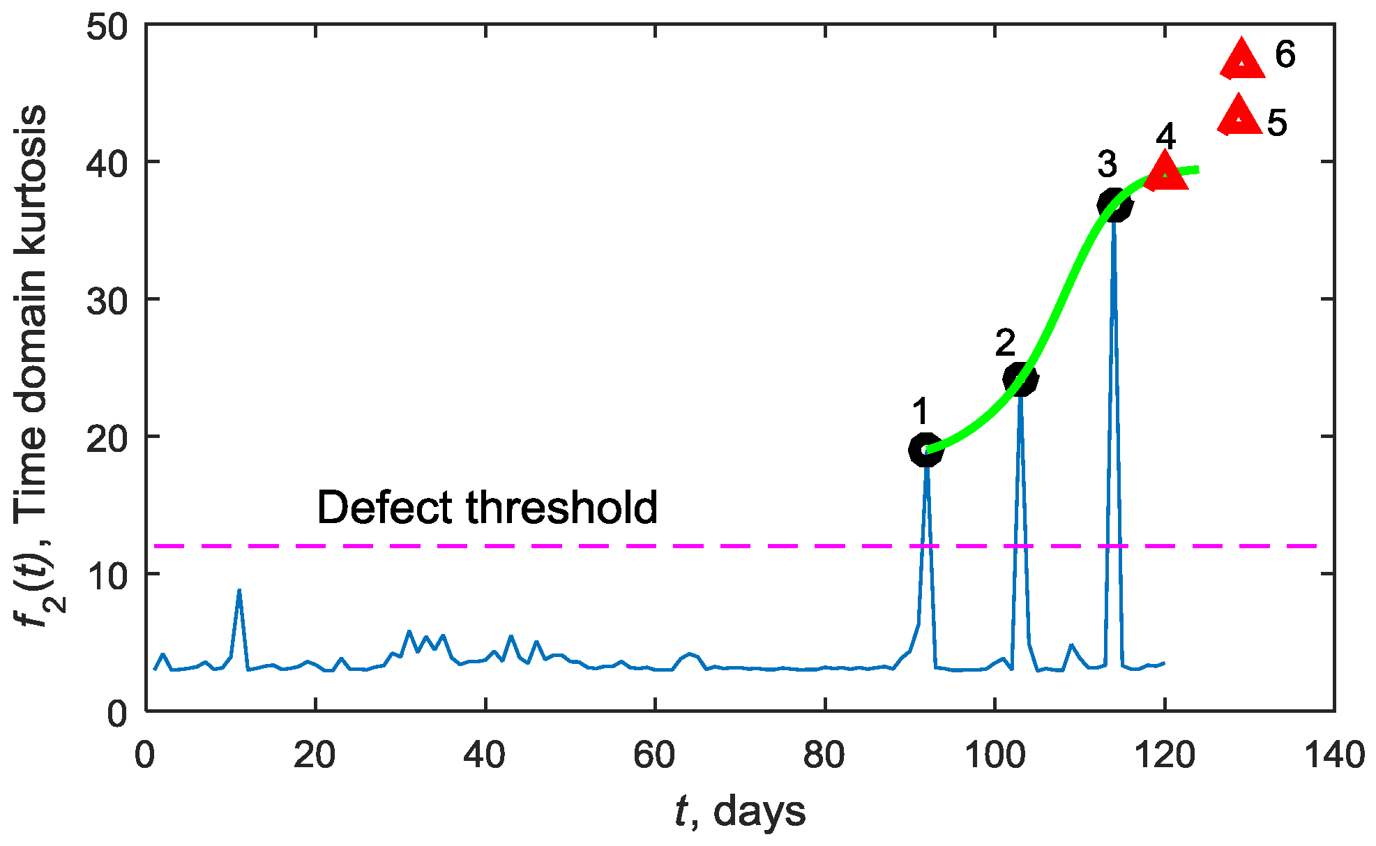
Firstly, three of the five features presented in Figure 2 are selected based on the evaluation criteria (described in Section 4.2). Once Step (1) has triggered the incipient defect, initial threshold is set-up. The initial threshold is set at four 4 times the kurtosis value of the normal bearing condition. In Step (2), the data point that exceeds the predetermined initial threshold of each selected feature is saved and used for prediction. From the laboratory slew bearing data, it was found that the minimum number of data points used for prediction is 3. Time-domain kurtosis is used as an illustration in Figure 4. The measurement day and the kurtosis level of the first three non-linear data points which exceed the threshold are presented in

Table 2. Non-linear data points.

Data Point	Measurement Day (Xj)	Feature Level (Yj)
A	92	19
B	103	24.12
C	114	36.83

where j represents points A, B or C.

. We refer these points as ‘non-linear’ data because the interval between one point and the next is not equal and the level of kurtosis does not always increase linearly.

Secondly, the non-linear regression model is built in 4 steps. (1) Calculate data point x_j with small step dx. dx equal to 0.2 is used throughout this paper. The result is the vector x; (2) Set the kernel width α. α for time-domain kurtosis prediction is 6. dx and α are selected by trial and error to get the optimum regression model; (3) Apply the Gaussian kernel to each data point X_j using the following equation

$$K_j(x,X_j)=\exp \left(-\frac{{(x-X_j)}^2}{2{\alpha }^2}\right)$$

(11)

where subscript j denotes non-linear data point. According to the example given in Table 2, X_j are X_A, X_B and X_C. (4) Compute the weight vector w = (w₁, w₂, …, w_p) using the least square method by minimizing the sum square error between predicted ${\widehat{Y}}_j$ and monitored $Y_j$ as follows:

$$\mathsf{\epsilon }={\displaystyle \sum _{j=1}^p({\widehat{Y}}_j-Y_j)}$$

(12)

where p is the number of non-linear data points to be regressed and predicted. In this example, p = 3. lsqcurvefit MATLAB function is used to obtain the weight vector w. The result of the non-linear regression model is presented in

Table 3. Kernel regression model for 1 step-ahead prediction of time-domain kurtosis.

Data Point (x-axis)	x	K1(x,XA)	K2(x,XB)	K3(x,XC)	w1 K1	w2 K2	w3 K3	${\displaystyle \sum _{\mathit{j}=1}^{\mathit{p}}{\mathit{w}}_{\mathit{j}}{\mathbf{K}}_{\mathit{j}}}$	${\displaystyle \sum _{\mathit{j}=1}^{\mathit{p}}{\mathbf{K}}_{\mathit{j}}}$	Data Point (y-axis)
XA = 92	92	1	0.186	0.0012	18.354	4.158	0.047	22.560	1.187	YA = 18.998
	92.2	0.999	0.197	0.0014	18.344	4.417	0.053	22.815	1.198	19.033
	92.4	0.997	0.210	0.0015	18.313	4.688	0.060	23.062	1.209	19.070
	.	.	.	.	.	.	.	.	.	.
	.	.	.	.	.	.	.	.	.	.
	.	.	.	.	.	.	.	.	.	.
	102.6	0.210	0.997	0.164	3.854	22.273	6.505	32.633	1.372	23.780
	102.8	0.197	0.999	0.175	3.632	22.310	6.927	32.869	1.372	23.949
XB = 103	103	0.186	1	0.186	3.418	22.322	7.367	33.109	1.372	YB = 24.122
	103.2	0.175	0.999	0.197	3.214	22.310	7.827	33.352	1.372	24.301
	103.4	0.164	0.997	0.210	3.018	22.273	8.307	33.599	1.372	24.484
	.	.	.	.	.	.	.	.	.	.
	.	.	.	.	.	.	.	.	.	.
	.	.	.	.	.	.	.	.	.	.
	113.6	0.0015	0.210	0.997	0.0282	4.688	39.466	44.183	1.209	36.535
	113.8	0.0014	0.197	0.999	0.0250	4.417	39.532	43.975	1.198	36.685
XC = 114	114	0.0012	0.186	1	0.0221	4.158	39.554	43.734	1.187	YC = 36.830
	114.2	0.0011	0.175	0.999	0.0195	3.909	39.532	43.461	1.175	36.968
	114.4	0.0009	0.164	0.997	0.0173	3.671	39.466	43.155	1.163	37.100
	.	.	.	.	.	.	.	.	.	.
	.	.	.	.	.	.	.	.	.	.
	.	.	.	.	.	.	.	.	.	.
	119.6	0.000025	0.021	0.646	0.00046	0.486	25.588	26.074	0.668	38.992
	119.8	0.000021	0.019	0.626	0.0004	0.442	24.790	25.233	0.646	39.025
${\widehat{X}}_D$ = 120	120	0.000018	0.018	0.606	0.00034	0.403	23.991	24.394	0.624	${\widehat{Y}}_D$ = 39.055

Note: w = [w₁; w₂; w₃] = [18.35; 22.32; 39.55].

and shown in Figure 5.

Thirdly, the future value of the feature is predicted. The predicted value of Y_j at future X_j is given by the kernel regression formula (also called Nadaraya-Watson kernel weighted average) [39] as follows:

$${\widehat{Y}}_j=\frac{{\displaystyle \sum _{j=1}^p{w}_j{K}_j}}{{\displaystyle \sum _{j=1}^p{K}_j}}$$

(13)

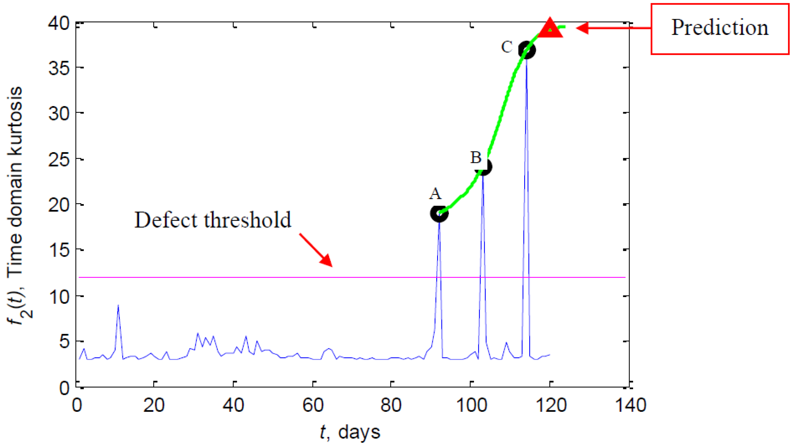
The one-step-ahead prediction of time-domain kurtosis is presented in Figure 6.

The result shown in Figure 6 is one-step-ahead prediction of time-domain kurtosis based on modified kernel regression method presented in Section 2.2. The modified kernel regression is proposed to calculate a model based on 3 points and predict one-point-ahead. This method can predict one-point-ahead of time-domain kurtosis feature based on 3 points with similar spacing between the points as illustrated in Figure 4. The proposed method still works although the spacing between 3 points is different.

3. Experimental Set-Up

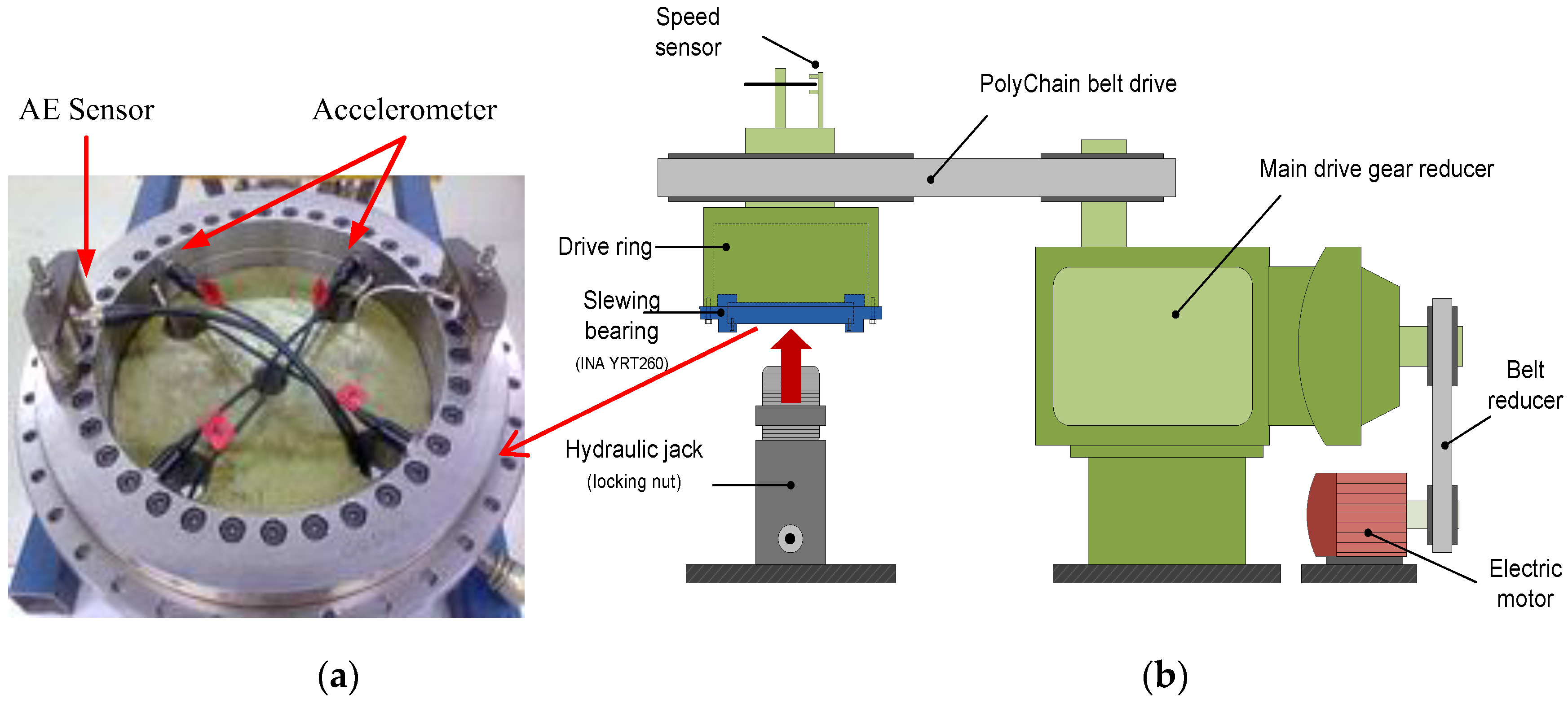
The vibration data of the accelerated wear test used in this paper was acquired from a laboratory slew bearing test rig shown in Figure 7. The schematic of the slew bearing test rig showing the main drive reducer, the hydraulic load and how the bearing is attached is shown in Figure 7a. A 30 tonnes axial load was hydraulically applied. The test rig was operated in continuous rotation at 1 rpm. The slew bearing used was INA YRT260 type axial/radial bearing with inner and outer diameter of 260 mm and 385 mm, respectively. The vibration data was acquired from four accelerometers installed on the inner radial surface at 90 degrees to each other (see Figure 7b) with 4880 Hz sampling rates. The accelerometers were IMI608 A11 ICP type sensors. The accelerometers were connected to a high speed Pico scope DAQ (PS3424). 139 days data were collected. In order to accelerate the damage and reduce the bearing service life, coal dust was injected into the bearing. In practice, especially in steel making companies, slew bearing is located in open air and exposed to dusty environment. To replicate this condition, coal dust was inserted in day 58.

4. Results and Discussion

4.1. Step (1) Detection of the Incipient Slew Bearing Defect Using MSET and SPRT

Twelve features were extracted from four different methods [31]. Not all features were sensitive to the change of the bearing condition. Consequently, the method only uses five of the most sensitive features as the input to the MSET. The five features were (1) kurtosis extracted from accelerometer signal, f₁(t); (2) kurtosis extracted from the piecewise aggregate approximation (PAA) combined with circular analysis, f₂(t); (3) kurtosis extracted from the wavelet decomposition, f₃(t); (4) kurtosis extracted from the EMD, f₄(t); and (5) LLE feature obtained from the largest Lyapunov exponent algorithm, f₅(t) [32]. The five features were extracted over the 139 days test period. The plot of the aforementioned features has been shown in Figure 2. These features are used to establish data matrix P. Thus, the dimension of data matrix P in Equation (1) is 5 by 139, where 5 is the number of features and 139 is the number of days.

To detect the incipient slew bearing defect (Step 1), the MSET algorithm calculates the normal residual matrix (R_N) and the residual matrix of monitored state (R_M) (see Figure 3). In Step (1), the following inputs are required: training matrix T, memory matrix D, remaining training matrix L and observation matrix P_obs. In this paper, T of 50 days was used. In the computation, the sizes of matrices, D and L have to be half of T i.e., 25 days each. The reason why 50 days was used is because coal dust was not injected until day 58. In other words, during the first 50 days, the vibration signal had been acquired when the condition of the bearing was still normal. In practice, matrix P_obs is obtained from daily observation or measurement. The number of measurement days from normal to failure has been set as 139 days. P_obs is the matrix from day 51 to day 139.

After D and L have been determined, the weight of normal state vector (w₁) is then calculated using Equation (3) by employing the Euclidean distance as the non-linear operator. Vector w₁ represents the weight of normal data points in the training data. w₁ is used to calculate the normal estimate matrix (L_est) using Equation (5). And the normal residual matrix (R_N) is estimated by taking the difference between L_est and L, as shown in Equation (7). It should be noted that prior to the calculation of the statistical properties, matrix R_N is normalized with a zero mean. This is necessary for the next process in the SPRT method because under normal bearing conditions the mean value of the normal residual matrix (R_N) is expected to be ≈0. The result of normalized matrix (R_N) is presented in

Table 4. Normalized R_N matrix.

Day 1	Day 2	Day 3	Day 4	Day 5	Day 6	Day 7	Day 8	Day 9	Day 10	Day 11	Day 12	Day 13
0.044	0.042	0.042	0.042	0.042	0.043	0.042	0.043	0.044	0.042	0.042	0.042	0.043
0.025	0.021	0.021	0.022	0.022	0.023	0.021	0.024	0.025	0.022	0.022	0.021	0.022
0.016	0.015	0.015	0.015	0.015	0.016	0.015	0.016	0.016	0.015	0.015	0.015	0.015
0.018	0.017	0.017	0.017	0.017	0.018	0.017	0.018	0.018	0.017	0.017	0.017	0.018
−0.955	−0.957	−0.957	−0.957	−0.957	−0.956	−0.957	−0.956	−0.955	−0.957	−0.957	−0.957	−0.957
Day 14	Day 15	Day 16	Day 17	Day 18	Day 19	Day 20	Day 21	Day 22	Day 23	Day 24	Day 25
0.043	0.042	0.043	0.043	0.042	0.043	0.044	0.042	0.042	0.042	0.042	0.042
0.022	0.021	0.023	0.023	0.022	0.023	0.024	0.021	0.021	0.022	0.022	0.021
0.015	0.015	0.016	0.016	0.015	0.016	0.016	0.015	0.015	0.015	0.015	0.015
0.018	0.017	0.018	0.018	0.017	0.018	0.018	0.017	0.017	0.018	0.018	0.017
−0.957	−0.957	−0.956	−0.956	−0.957	−0.956	−0.955	−0.957	−0.957	−0.957	−0.957	−0.957

. A similar procedure is also employed to obtain the residual matrix of monitored state (R_M). Equation (4) is used to calculate the weight of monitored state vector (w₂), Equation (6) is then used to calculate the estimate matrix of monitored state (L_est) and Equation (8) to calculate the residual matrix of monitored state (R_M). Matrix R_M is then normalized within a range between maximum value and minimum value of the normalized normal residual matrix (R_N). The calculation of R_N and R_M is the final step of MSET. Both results are then fed into the SPRT.

In SPRT, statistical characteristics such as mean value, standard deviation and the range between maximum and minimum values are calculated from each column of normalized matrix R_N. These statistical properties belong to the normal condition of the bearing are used as the reference normal data. These properties also form the set of hypotheses in SPRT. For the monitored state, prior to the calculation of the mean value and the standard deviation, the matrix (R_M) is normalized within the range between maximum and minimum value of the normal state. The mean and standard deviation values of the normal state (up to days 25) are presented in

Table 5. Mean (M) values of normal state.

Day 1

Day 2

Day 3

Day 4

Day 5

Day 6

Day 7

Day 8

Day 9

Day 10

Day 11

Day 12

Day 13

−0.169

−0.172

−0.172

−0.171

−0.171

−0.171

−0.172

−0.170

−0.170

−0.171

−0.171

−0.172

−0.171

Day 14

Day 15

Day 16

Day 17

Day 18

Day 19

Day 20

Day 21

Day 22

Day 23

Day 24

Day 25

−0.171

−0.172

−0.170

−0.171

−0.171

−0.171

−0.170

−0.172

−0.172

−0.171

−0.171

−0.172

Note: M_min = −0.172, M_max = −0.169.

and

Table 6. Standard deviation (σ_normal) values of normal state.

Day 1	Day 2	Day 3	Day 4	Day 5	Day 6	Day 7	Day 8	Day 9	Day 10	Day 11	Day 12	Day 13
0.439	0.439	0.439	0.439	0.439	0.439	0.439	0.439	0.439	0.439	0.439	0.439	0.439
Day 14	Day 15	Day 16	Day 17	Day 18	Day 19	Day 20	Day 21	Day 22	Day 23	Day 24	Day 25
0.439	0.439	0.439	0.439	0.439	0.439	0.439	0.439	0.439	0.439	0.439	0.439

, respectively. The detection of the incipient slew bearing defects is obtained by comparing the statistical characteristics, the mean value and the standard deviation) of the monitored state to the statistical characteristics of the normal state.

This comparison is repeated to the 51 to 139 columns of the P_obs matrix. If the mean value or the standard deviation in each day lies outside the range of the reference mean values (Table 5) or standard deviation values (Table 6), incipient defect is considered to have occurred. This step is part of the SPRT procedure. To make a comparison, the list of hypotheses must be determined first including the normal condition (H₀) represented by mean value = M_normal and the standard deviation = σ_normal. Alternatives hypotheses H₁ to H₄ indicate the abnormal conditions. The set of hypotheses is given in Table 1.

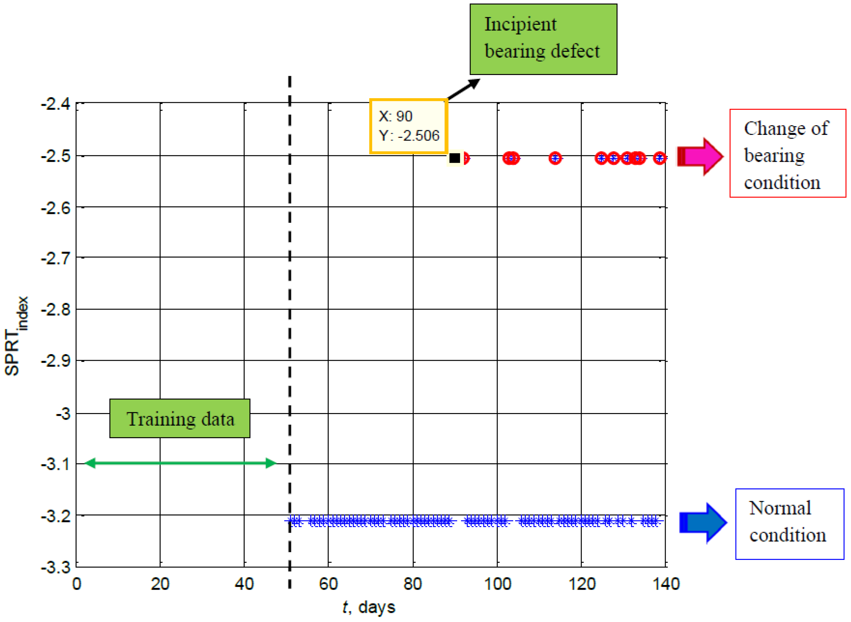
To measure the comparison mathematically, the ratio of the probability of alternative hypotheses (H₁ to H₄) and the probability of the null hypothesis (H₀) is calculated, Equation (10). Once probability ratio L_i is obtained, the SPRT index can be calculated by taking the natural logarithm of probability ratio L_i. The result of Step (1) is presented in Figure 8. It can be seen from the monitored data of day 51 to day 89 that the bearing is still in normal condition. The impending deterioration of the bearing is identified on day 90. Note that the impending deterioration is needed in Step (2) to predict the future state and to estimate the RUL estimation. A sample calculation of L_i for a day (day 51 and day 90) is presented in

Table 7. Example calculation of L_i in one day observation.

Dayth Observation	p({Si}/H)	p({Si}/H0)	Li (Equation (10))
day 51	0.04	0.99	−3.209
day 90	0.08	0.98	−2.506

Note: p({S_i}/H) is probability of statistical properties {S_i} given H is true and p({S_i}/H) is probability of statistical properties {S_i} given H₀ is true.

. When the condition of the bearing is still normal, the probability of statistical properties {S_i} that fall within the hypotheses H (p({S_i}/H)) is much lower than the probability of statistical properties {S_i} of the null hypothesis H₀ (p({S_i}/H₀)). To illustrate the normal condition (i.e., day 50), the natural logarithmic of L_i is given in Table 7 and shown in Figure 8. On the contrary, on day 90 the condition of the bearing started to deteriorate, the probability of statistical properties {S_i} that fall within the hypotheses H (p({S_i}/H)) will increase and the probability of statistical properties {S_i} that fall in the null hypothesis H₀ (p({S_i}/H₀)) will decrease, the natural logarithmic is then given in Table 7 and shown in Figure 8.

4.2. Step (2) Prediction of the Future State of Selected Features Using Kernel Regression

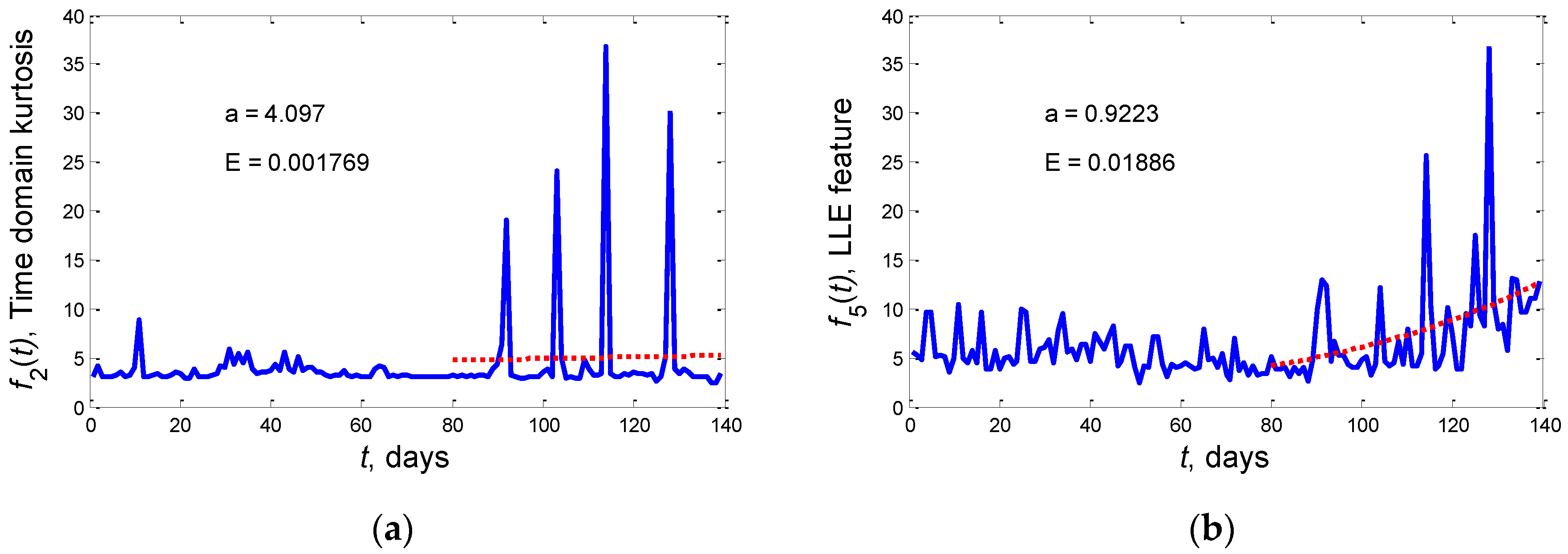
Features extracted from slew bearing vibration signals have different characteristic to those extracted from accelerometers signals of typical rolling element bearings. In typical rolling element bearings, when the bearing condition deteriorates, the features values increase gradually. In slew bearings, the changes of the slew bearing condition can be detected from a sharp increase of feature value. However, this value does not increase steadily as it does in typical high speeds roller bearings. The extracted features of the slew bearing signal usually revert to the normal level and rise again as the condition has deteriorated significantly. This condition is referred as ‘self-healing’ characteristic [41]. This is one of the difficulties in defect prediction especially for data-driven prognosis methods [42,43,44]. In this paper, the problem has been overcome using kernel regression. Prior to the use of kernel regression, all features have to be evaluated. Caesarendra et al. [32] presented four evaluation criteria to track the progressive bearing defect. In the present study, another evaluation criterion based on exponential function is proposed. It is well known that as bearing deteriorates, certain features will increase exponentially. Hence, an evaluation criterion (E) obtained from the coefficient of the exponential curve fitting of the feature being evaluated is used as illustrated below. Suppose f(t) is the monitored evaluation function.

$$f(t)=a{e}^{(Et)}$$

(14)

where a and E are the curve fitting exponential coefficients, and t is the measurement days. The calculation of E for the time-domain kurtosis feature and the LLE feature is presented in Figure 9. The two figures show clearly that the LLE feature shows a greater exponential increasing trend than the time-domain kurtosis feature. The dotted line in Figure 9a,b is the exponential curve fitted from day 80 to day 139.

In Step (2), kernel regression is employed to predict the future bearing condition and to estimate the RUL of the slew bearing. This prediction starts when there is warning of impending deterioration of the bearing condition. The basic kernel regression algorithm is improved by adding a k-step-ahead subroutine. At each k-step, non-linear regression model and posterior (predicted) point is estimated and updated. The purpose of this process is to estimate a one-step-ahead prediction of the kernel regression model based on past non-linear data points.

Kernel regression is an effective method to build a model from non-linear data. The process is done by taking the highest data point of the current kernel regression model and then using it as the next data point (e.g., predict the 4th data point if the initial model is built from three data points). The new data point is then used to build a new kernel regression model and estimate the next data point. The process is repeated until the specified k-step-ahead prediction is reached. To illustrate the process, a time domain kurtosis feature is used as the monitored parameter being predicted.

Kurtosis is selected as an input of kernel regression because it has a certain value for normal bearing condition and the kurtosis value for defect condition. This is necessary for the detection of incipient defect in Step (1), which is set with the predetermined warning threshold and for prediction in Step (2), which is set with the damage bearing threshold. The kurtosis value for normal bearing signals is approximately 3 [40]. The increase of this value indicates that the bearing condition has changed. Some research mentioned that the kurtosis value will reach about 50 when high impact occur [45]. Aye [46] studied the kurtosis of normal and faulty tapered bearings running at speed between 409 RPM and 1200 RPM. It has been found that the kurtosis value for normal bearings is 2.89. Surprisingly, the kurtosis value for faulty bearings with 409 RPM increases significantly to about 30.26 and for 1200 RPM drops to 1.23. The same author [46] demonstrated that the kurtosis value of bearing damage with low rotational speed (low RPM) can be much higher than the normal value. Guo et al. [47] presented a method for recovering the bearing signal from large noisy signal using a hybrid method based on spectral kurtosis and ensemble EMD. It was found that the kurtosis value of each bearing fault condition was recovered and identified more easily. For instance, the kurtosis value of a bearing with an inner race defect and a ball defect is 18.35 and 41.20, respectively.

Supposed 3 points are available denoted as point 1, 2, and 3 as shown in Figure 10. Firstly, the method predict one-step-ahead of degradation parameter denoted as point 4 (red triangle) based on 3 points i.e., point 1, 2 and 3. Secondly, to predict next degradation parameter denoted as point 5, the method used point 2, 3 and 4. Thirdly, to predict point 6 the method used point 3, 4 and 5. According to the Figure 10, the plotted curve shows an increasing trend, it is due to the first 3 points used has an increasing trend. Thus for next prediction the method employed both actual value and predicted value to predict the next degradation parameter. In practice, when the kurtosis value is acquired from online condition monitoring, the points can be replaced by actual kurtosis value. The method will use 3 updated kurtosis values to do one-step-ahead prediction.

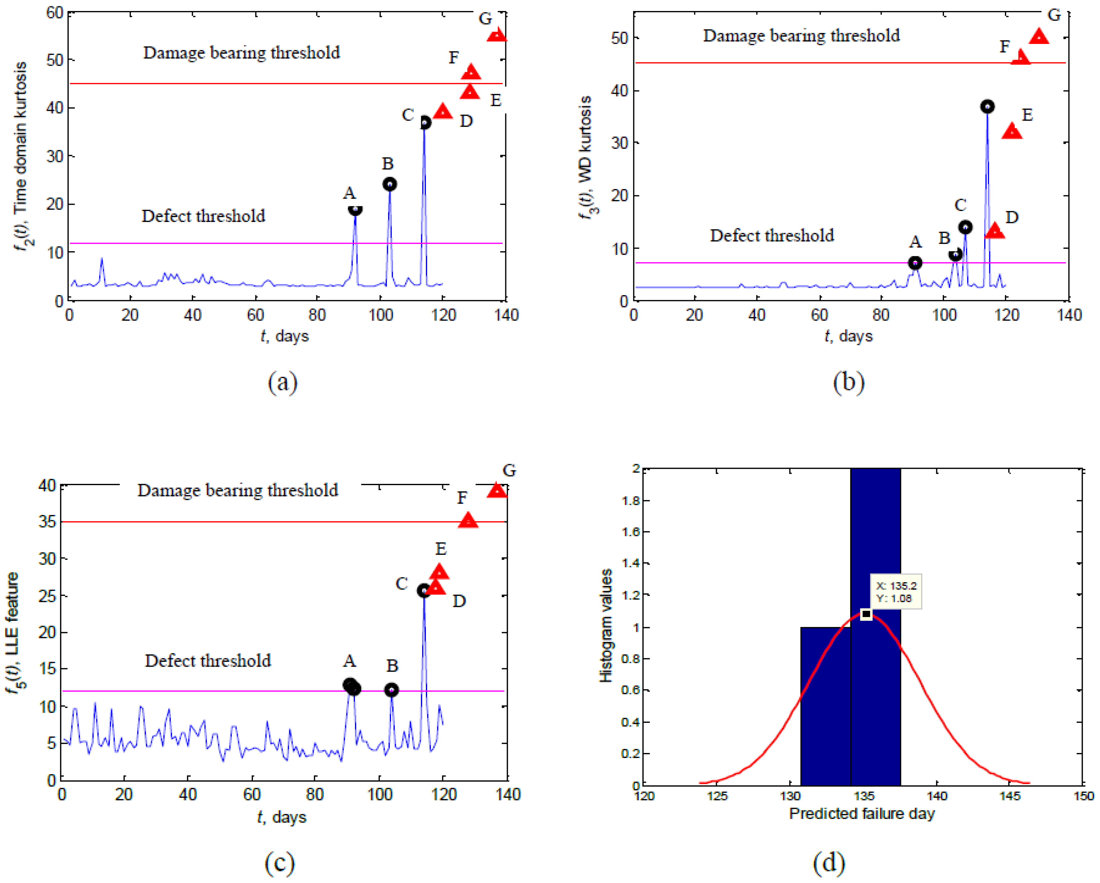
Setting a threshold level are depends on the different situations and types of bearings. The information can be obtained from the maintenance engineer or past condition monitoring (CM) data with has similar type of bearing and load condition. As has been done in past works [45,46,47], we have set the threshold kurtosis value of 45 for the time-domain kurtosis and the WD feature, while the threshold for the LLE feature is set at 35. The proposed kernel regression method was applied up to 120 days, as by day 120 the kurtosis value has exceeded 4 times the normal value and three data points greater than the alarm threshold level have been detected. It should be noted that three data points is the minimum requirement in the initial kernel regression model. Note that the levels of the three selected features up to day 120 are still below the bearing damage threshold of 45. The predictions of the kernel regression of the three features mentioned above are presented in Figure 11a–c. The four step-ahead of kernel regression are used (k = 4) and thus the 4 step-ahead predicted data points are shown with ‘Δ’ symbol, while ‘o’ represents the actual value. It can be seen that the predicted future values increases. When the data point exceeds the damage threshold level, the last predicted day is noted and used to estimate the histogram of final failure. Once the histogram of final failure is obtained, the RUL can be easily estimated by taking the difference between the predicted final failure time and the last measurement day (the last measurement day is 120).

Based on this analysis, the predicted failure day of the bearing is shown to be dependent on the features and summarized in

Table 8. The prediction of failure day.

Feature	nth Day Failure (x-axis)	Feature Level (y-axis)	Threshold
Time-domain kurtosis	137.6	55	45
WD kurtosis	130.8	46	45
LLE feature	137	39	35

. Detail information of the three non-linear data used to build the initial model and the predicted data point of the modified kernel regression method for each feature is shown in

Table 9. Original non-linear data points and predicted data points of time domain kurtosis.

Data Point	Measurement Day	Feature Value
A	92	19
B	103	24.12
C	114	36.83
D	120	39
E	128.6	43
F	129.2	47
G	137.6	55

,

Table 10. Original non-linear data points and predicted data points of WD kurtosis.

Data Point	Measurement Day	Feature Value
A	91	7.24
B	104	8.84
C	107	14
D	116.4	13
E	122.2	32
F	125	46
G	130.8	50

and

Table 11. Original non-linear data points and predicted data points of LLE feature.

Data Point	Measurement Day	Feature Value
A	92	12.36
B	104	12.22
C	114	25.69
D	117.8	26
E	118.8	28
F	128	35
G	137	39

(point A–D). It is shown in Figure 11b,c is the WD kurtosis feature and LLE feature, respectively. For WD kurtosis feature the spacing is different (day 104th − day 91th = 13 days and day 107th − day 104th = 3 days). The LLE Feature also has different spacing (day 104th − day 92th = 12 days and day 114th − day 104th = 10 days). Points D–G are the predicted features values. These points are estimated based on the 4-step-ahead prediction of the kernel regression. According to the results in Table 9, Table 10 and Table 11, the y-axis values of the fourth predicted points exceed the bearing damage threshold. The day of each fourth predicted point (point G) is noted as the final failure of the slew bearing. Three predicted days (point G) are then inputted to the histogram. The result of this is presented in Figure 11d. It should be noted that with more features used, the more accurate the distribution fit of the histogram will be. It can be seen from Figure 11d that the predicted final failure is day 135. Further, the RUL of the bearing can be estimated by taking the difference between the predicted failure day and the last measurement day i.e., 135 − 120 = 15 day. The final failure histogram was calculated using a common MATLAB function ‘histfit’. The probability curve is plotted based on the predicted final failure from three methods: (a) time-domain kurtosis at 137.6 day; (b) WD kurtosis at 130.8 day; and (c) LLE feature at 137 day.

During the slew bearing lab experiment, complete failure is unpredictable. When a burst vibration signal on day 141 was detected, the test-rig had to be shut down. To inspect the damage and verify the result of the proposed prognosis method, the slew bearing was dismantled and inspected. Some of the defective rollers and outer race can be clearly seen in Figure 12. The actual final failure day of lab slew bearing is considered one day before the severe burst vibration signal i.e., day 140. The accuracy of prediction is estimated as follows:

$$A_p=\left(1-\frac{\left|t_a-t_p\right|}{t_a}\right)\times 100\%=\left(1-\frac{\left|140-135\right|}{140}\right)\times 100\%=96.43\%$$

(15)

where t_a is actual final failure day and t_p is predicted failure day.

5. Conclusions

An integrated condition monitoring and prognosis method of low speed slew bearing has been presented. The method employs combined MSET and SPRT to detect the incipient bearing defect, and kernel regression to predict the future state and to estimate the RUL. The method has been implemented in the monitoring and prediction of laboratory slew bearing condition, where the test was run with new bearing condition until failure. Combined MSET and SPRT method was used to analyse the vibration features calculated from the accelerometer data of 139 days measurement. Based on the set of hypothesis in SPRT method, it was found that the incipient defect of slew bearing occurred in day 90. After the incipient defect was detected, the kernel regression calculation started to predict the future state. To validate the method, 120 measurement days were analysed. The predicted of failure days were constructed and the final failure day (day 135) was predicted based on the peak of the normal distribution fit of the histogram. The RUL was estimated by to be 15 days (135 − 120 days).

References

1. Henao, H.; Capolino, G.-A.; Fernandez-Cabanas, M.; Filippetti, F.; Bruzzese, C.; Strangas, E.; Pusca, R.; Estima, J.; Riera-Guasp, M.; Hedayati-Kia, S. Trends in fault diagnosis for electrical machines: A review of diagnostic techniques. IEEE Ind. Electron. Mag. 2014, 8, 31–42. [Google Scholar] [CrossRef]
2. Frosini, L.; Harlişca, C.; Szabó, L. Induction machine bearing fault detection by means of statistical processing of the stray flux measurement. IEEE Trans. Ind. Electron. 2015, 62, 1846–1854. [Google Scholar] [CrossRef]
3. Rodgers, L.M. The application of vibration signature analysis and acoustic emission source location to on-line condition monitoring of anti-friction bearings. Tribol. Int. 1979, 12, 51–58. [Google Scholar] [CrossRef]
4. Žvokelj, M.; Zupan, S.; Prebil, I. Multivariate and multiscale monitoring of large-size low-speed bearings using ensemble empirical mode decomposition method combined with principal component analysis. Mech. Syst. Signal Process. 2010, 24, 1049–1067. [Google Scholar] [CrossRef]
5. Qiu, H.; Lee, J.; Lin, J.; Yu, G. Wavelet filter-based weak signature detection method and its application on rolling element bearing prognostics. J. Sound Vib. 2006, 289, 1066–1090. [Google Scholar] [CrossRef]
6. Zhu, X.; Zhang, Y.; Zhu, Y. Bearing performance degradation assessment based on the rough support vector data description. Mech. Syst. Signal Process. 2013, 34, 203–217. [Google Scholar] [CrossRef]
7. Lu, C.; Tao, L.; Fan, H. An intelligent approach to machine component health prognostics by utilizing only truncated histories. Mech. Syst. Signal Process. 2014, 42, 300–313. [Google Scholar] [CrossRef]
8. Lei, Y.; Li, N.; Gontarz, S.; Lin, J.; Radkowski, S.; Dybala, J. A model-based method for remaining useful life prediction of machinery. IEEE Trans. Reliabil. 2016, 65, 1314–1326. [Google Scholar] [CrossRef]
9. Li, N.; Lei, Y.; Lin, J.; Ding, S.X. An improved exponential model for predicting remaining useful life or rolling element bearings. IEEE Trans. Ind. Electron. 2015, 62, 7762–7773. [Google Scholar] [CrossRef]
10. Žvokelj, M.; Zupan, S.; Prebil, I. Non-linear multivariate and multiscale monitoring and signal denoising strategy using kernel principal component analysis combined with ensemble empirical mode decomposition method. Mech. Syst. Signal Process. 2011, 25, 2631–2653. [Google Scholar] [CrossRef]
11. Lin, T.R.; Kim, E.; Tan, A.C.C. A practical signal processing for condition monitoring of low speed machinery using peak-hold-down-sample algorithm. Mech. Syst. Signal Process. 2013, 36, 256–270. [Google Scholar] [CrossRef]
12. Singer, R.M.; Gross, K.C.; Herzog, J.P.; King, R.W.; Wegerich, S.W. Model-based nuclear power plant monitoring and fault diagnosis: Theoretical foundations. In Proceedings of the 9th International Conference on Intelligent Systems Applications to Power Systems, Seoul, Korea, 6–10 July 1997. [Google Scholar]
13. Gross, K.C.; Singer, R.M.; Wegerich, S.W.; Herzog, J.P. Application of a model-based fault detection system to nuclear plant signals. In Proceedings of the 9th International Conference on Intelligent Systems Applications to Power Systems (ISAP’97), Seoul, Korea, 6–10 July 1997. [Google Scholar]
14. Zavaljevski, N.; Gross, K.C. Sensor fault detection in nuclear power plants using multivariate state estimation technique and support vector machine. In Proceedings of the 3rd International Conference of the Yugoslav Nuclear Society YUNSC 2000, Belgrade, Yugoslavia, 2–5 October 2000. [Google Scholar]
15. Gribok, A.V.; Urmanov, A.M.; Hines, J.W. Uncertainty analysis of memory based sensor validation techniques. Real-Time Syst. 2004, 27, 7–26. [Google Scholar] [CrossRef]
16. Cheng, S.; Pecht, M. Multivariate state estimation technique for remaining useful life prediction of electronic product. In Proceedings of the Association for the Advancement of Artificial Intelligence, Vancouver, BC, Canada, 22–26 July 2007; pp. 26–32. [Google Scholar]
17. Peng, J.; Xiao, W.D.; Huang, X.P. A health monitoring method based on multivariate state estimation technique. Appl. Mech. Mater. 2013, 281, 80–85. [Google Scholar] [CrossRef]
18. Yongjie, Z.; Dongfeng, W.; Junying, Z.; Yuejiao, H. Research on early fault diagnostic method of wind turbines. Telkomnika 2013, 11, 2330–2341. [Google Scholar] [CrossRef]
19. Caesarendra, W.; Lee, J.M.; Ha, J.M.; Choi, B.K. Slew bearing early damage detection based on multivariate state estimation technique and sequential probability ratio test. In Proceedings of the 2015 IEEE International Conference on Advanced Intelligent Mechatronics (AIM), Busan, Korea, 7–11 July 2015. [Google Scholar]
20. Wald, A. Sequential test of statistical hypotheses. Ann. Math. Stat. 1945, 16, 117–186. [Google Scholar] [CrossRef]
21. Wald, A. Sequential Analysis; John Wiley and Sons: New York, NY, USA, 1947. [Google Scholar]
22. Pecht, M.; Jaai, R. A prognostics and health management roadmap for information and electronics-rich-systems. Microelectron. Reliabil. 2010, 50, 317–323. [Google Scholar] [CrossRef]
23. Gross, K.C.; Humerik, K.E. Sequential probability ratio tests for nuclear plant component surveillance. Nuclear Technol. 1991, 93, 131–137. [Google Scholar]
24. Sohn, H.; Allen, D.W.; Worden, K.; Farrar, C.R. Statistical damage classification using sequential probability ratio tests. Struct. Health Monit. 2003, 2, 57–74. [Google Scholar] [CrossRef]
25. Jarman, K.D.; Smith, L.E.; Carlson, D.K. Sequential probability ratio test for long-term radiation monitoring. IEEE Trans. Nuclear Sci. 2004, 50, 1662–1666. [Google Scholar] [CrossRef]
26. Chen, H.; Shang, Y.; Sun, K. Multiple fault condition recognition of gearbox with sequential hypothesis test. Mech. Syst. Signal Process. 2013, 40, 469–482. [Google Scholar] [CrossRef]
27. Gross, K.C.; Lu, W. Early detection of signal and process anomalies in enterprise computing systems. In Proceedings of the 2002 IEEE International Conference on Machine Learning and Applications (ICMLA), Las Vegas, NV, USA, 24–27 June 2002. [Google Scholar]
28. Niu, G.; Zhao, Y.; Defoort, M.; Pecht, M. Fault diagnosis of locomotive electro-pneumatic brake through uncertain bond graph modeling and robust online monitoring. Mech. Syst. Signal Process. 2015, 50–51, 676–691. [Google Scholar] [CrossRef]
29. López-Rubio, E.; Florentín-Núnez, M.N. Kernel regression based feature extraction for 3D MR image denoising. Med. Image Anal. 2011, 15, 498–513. [Google Scholar] [CrossRef] [PubMed]
30. Takeda, H.; Farsiu, S.; Milanfar, P. Kernel regression for image processing and reconstruction. IEEE Trans. Image Process. 2007, 16, 349–366. [Google Scholar] [CrossRef] [PubMed]
31. Jones, M.C.; Park, H.; Shin, K.I.; Vines, S.K.; Jeong, S.O. Relative error prediction via kernel regression smoothers. J. Stat. Plan. Inference 2008, 138, 2887–2898. [Google Scholar] [CrossRef]
32. Caesarendra, W.; Kosasih, B.; Tieu, A.K.; Moodie, C.A.S. Circular domain features based condition monitoring for low speed slewing bearing. Mech. Syst. Signal Process. 2014, 45, 114–138. [Google Scholar] [CrossRef]
33. Caesarendra, W.; Kosasih, B.; Tieu, A.K.; Moodie, C.A.S. Application of the largest Lyapunov exponent algorithm as a feature extraction method for low speed slew bearing condition monitoring. Mech. Syst. Signal Process. 2015, 50–51, 116–138. [Google Scholar] [CrossRef]
34. Black, C.L.; Uhrig, R.E.; Hines, J.W. System modelling and instrument calibration verification with a nonlinear state estimation technique. In Proceedings of the Maintenance and Reliability Conference (MARCON), Knoxville, TN, USA, 12–14 May 1998. [Google Scholar]
35. Cheng, S.; Tom, K.; Thomas, L.; Pecht, M. A wireless sensor system for prognostics and health management. IEEE Sens. J. 2010, 10, 856–862. [Google Scholar] [CrossRef]
36. Atkeson, C.G.; Moore, A.W.; Schaal, S. Locally weighted learning. Artif. Intell. Rev. 1997, 11, 11–73. [Google Scholar] [CrossRef]
37. Nadaraya, E.A. On estimating regression. Theory Probab. Its Appl. 1964, 9, 141–142. [Google Scholar] [CrossRef]
38. Watson, G.S. Smooth regression analysis. Indian J. Stat. Ser. A 1964, 26, 359–472. [Google Scholar]
39. Teknomo, Kardi (2007) Kernel Regression. Available online: http://people.revoledu.com/kardi/tutorial/Regression/kernelregression/ (accessed on 27 February 2017).
40. Caesarendra, W.; Widodo, A.; Yang, B.S. Application of relevance vector machine and logistic regression for machine degradation assessment. Mech. Syst. Signal Process. 2010, 24, 1161–1171. [Google Scholar] [CrossRef]
41. Moodie, C.A.S. An Investigation into the Condition Monitoring of Large Slow Speed Slew Bearings. Ph.D. Thesis, University of Wollongong, Wollongong, Australia, 2009. [Google Scholar]
42. Caesarendra, W.; Widodo, A.; Yang, B.S. Combination of probability approach and support vector machine towards machine health prognostics. Probab. Eng. Mech. 2011, 26, 165–173. [Google Scholar] [CrossRef]
43. Caesarendra, W.; Widodo, A.; Thom, P.H.; Yang, B.S.; Setiawan, J.D. Combined probability approach and indirect data-driven method for bearing degradation prognostics. IEEE Trans. Reliab. 2011, 60, 14–20. [Google Scholar] [CrossRef]
44. Niu, G.; Yang, B.S. Dempster-Shafer regression for multi-step-ahead time-series prediction towards data-driven machinery prognosis. Mech. Syst. Signal Process. 2009, 23, 740–751. [Google Scholar] [CrossRef]
45. De Lorenzo, F.; Calabro, M. Kurtosis: A statistical approach to identify defect in rolling bearing. In Proceedings of the 2nd International Conference on Marine Research and Transportation, Ischia Naples, Italy, 28–30 June 2007; pp. 17–24. [Google Scholar]
46. Aye, S.A. Statistical approach for tapered bearing fault detection using different methods. In Proceedings of the World Congress on Engineering (WCE) 2011, London, UK, 6–8 July 2011; Vol III. [Google Scholar]
47. Guo, W.; Tse, P.W.; Djordjevich, A. Faulty bearing signal recovery from large noise using a hybrid method based on spectral kurtosis and ensemble empirical mode decomposition. Measurement 2012, 45, 1308–1322. [Google Scholar] [CrossRef]
Figure 1. The integrated condition monitoring and prognosis method for low speed slew bearing.
Machines 05 00011 g001
Figure 2. (a) circular kurtosis [32]; (b) time-domain kurtosis [32]; (c) wavelet kurtosis [32]; (d) EMD kurtosis [32]; (e) the LLE feature [33]. Note: t = dayth.
Machines 05 00011 g002aMachines 05 00011 g002b
Figure 3. Flowchart of the proposed combined MSET and SPRT method in step (1).
Machines 05 00011 g003
Figure 4. Kurtosis extracted from the original vibration signal. The well-known kurtosis value for normal bearing is 3 [40]. The alarm threshold is set at 4 × 3 = 12.
Machines 05 00011 g004
Figure 5. Regression model of three data points and one-step-ahead prediction.
Machines 05 00011 g005
Figure 6. One-step-ahead prediction of time-domain kurtosis feature.
Machines 05 00011 g006
Figure 7. (a) Sensor attachment; (b) Schematic of laboratory slew bearing test rig.
Machines 05 00011 g007
Figure 8. The SPRT index result for detecting impending bearing deterioration.
Machines 05 00011 g008
Figure 9. Evaluation criterion (E) calculation: (a) time domain kurtosis feature; (b) LLE feature.
Machines 05 00011 g009
Figure 10. Kernel regression model and three-step-ahead prediction.
Machines 05 00011 g010
Figure 11. Prediction of modified Kernel regression: (a) Time-domain kurtosis; (b) Wavelet kurtosis; (c) LLE feature; (d) PDF of the predicted failure day of the slew bearing. 135.2 is the peak value of the normal distribution.
Machines 05 00011 g011
Figure 12. Slew bearing damage: (a) A view of damaged rollers in the axial plane; (b) Outer raceway damage.
Machines 05 00011 g012