Calculation of the Incompressible Viscous Fluid Flow in Piston Seals of Piston Hybrid Power Machines

Abstract

The article considers the calculation of the flow of a viscous incompressible fluid in piston seals of piston hybrid power machines. The most widely used and effective seals are considered: a smooth gap seal and a step-type gap seal, and—based on the references analyses—the initial boundary conditions for their calculation are determined. The laminar and turbulent flows in gap seals are calculated based on the well-known analytical relationships, experimental studies and flow models, including the k-ε, Menter’s Shear StressTransport (SST) and Reynolds Stress (RSM) turbulence models. The effectiveness of using each model to determine average velocities, flow rates, and velocity plots in the cross section of a gap seal, as well as the adequacy of the description of known physical laws, is estimated. The results proved that the RSM turbulence model is better for the gap seals of different types under different modes of motion.

1. Introduction

Considerable energy is spent on the drive of piston compressors and piston pumps, including radial piston and axial piston, considering their widespread use in the automotive, machine-tool, aviation and other industries. As a result, the task of increasing their efficiency and effectiveness is not new, but still relevant and timely.

One of the main ways to increase dramatically the efficiency and economy of gas compression is to combine a piston compressor with a piston pump and to obtain a piston hybrid power machine (PHPM) in which gas and liquid are compressed and moved by changing the volume of the working chambers (see Figure 1). Due to the intensive cooling of the suction and compressed gas and the elimination of leaks and leakage losses, the indicator efficiency increases and work is reduced; by eliminating dead space in the compressor section by filling it with fluid, the feed coefficient and productivity of the compressor section are increased; due to the fluid in the gap seal, the work of friction forces in the cylinder-piston group decreases; due to leakage of liquid into the working cavity of the pump section from the gap in the piston seal, the cavitation reserve increases [1].

Thus, the piston seal through which the fluid flows from the pump section to the compressor section and back is a key factor providing all positive effects in the PHPM.

Over the years, gap seals have been heavily used in hydraulic, oil, and fuel systems, as well as in pumps, hydraulic motors, distribution and control devices, and power cylinders.

Its widespread use is due to constructive simplicity and efficiency. A gap seal is a gap between two mating parts in the simplest case. There is fluid flow observed in the gap seal under the action of a pressure differential between the sealing cavity and the low-pressure cavity. There will be two flow modes observed: laminar and turbulent, depending on the pressure drop, physical properties of the fluid and the geometrical dimensions of the gap seal.

In the general case, the gap between the two mating parts can be straight, expanding, tapering and of another shape, with and without labyrinth grooves.

Analytical solutions have been obtained for the distribution of the diagrams of velocities, average velocity and flow rate for the laminar flow in the simplest slots. So, formulas for determining the flow rate were obtained for flat and annular slots, called Hagen–Poiseuille formulas [2]. In the general case, the Navier-Stokes equation and the continuity equation are used to describe the laminar flow in the gaps [3,4]. Due to the fact that solving complete Navier-Stokes equations causes great mathematical difficulties, the equations are simplified by introducing the following assumptions:

-

fluid flow is steady, isothermal between solid impermeable walls;

-

the mass terms of the equation of motion are negligible (they should be taken into account only when the fluid flows on a free surface or when the fluid density is inhomogeneous);

-

inertia forces are also negligible [4,5] (inertia forces can be neglected if the reduced Reynolds number is $R{e}^{\ast }=\frac{vl}{\nu }{\left(\frac{h}{l}\right)}^2\le 1$, where $v$ is determining speed; $\nu$ is kinematic viscosity; $l$ is seal length; $h$ is slot height);

-

$\frac{{\partial }^2{v}_x}{\partial x^2}$ value is less then $\frac{{\partial }^2{v}_x}{\partial y^2}$ value and it can be neglected;

-

transverse pressure gradient is negligible;

-

all members containing $z$ coordinate (coordinate in the transverse direction) and derivatives with respect to $z$ are discarded.

As a result of the assumptions made, the system of equations is significantly simplified and can be used to obtain analytical solutions.

Analytical calculation is impossible in a turbulent fluid flow, which was not an overcome problem for their calculation with a Reynolds number more than 1000.

Currently, due to the development of computer technology and numerical methods of analysis, two-parameter semi-empirical turbulence models using Reynolds averaging and turbulent viscosity are widely used. These models include $k-\epsilon$, $k-\omega$ and combinations thereof, for example $SST$ [6,7,8,9,10,11,12,13]. There are also many other turbulence models based on an additional tensor in the Reynolds equations, which includes so-called Reynolds stresses. A detailed analysis of turbulence models will be given in the article below when considering turbulent flow.

It should be noted that all developed models require experimental verification. The article will also present the results of experimental studies.

Thus, the main objectives of this article can be formulated as follows:

• To analyze gap seals used in hybrid power machines and select the most structurally simple from them and effective in operation.
• To determine the basic geometric and operational parameters for the selected types of gap seals.
• To determine the flow patterns in them based on existing recommendations.
• To calculate the laminar and turbulent flow modes. To determine the most suitable turbulence models for the turbulent flow mode and conduct a comparative analysis of the effectiveness of their application based on a comparison with the results of experimental studies and known physical concepts.

To provide recommendations on the applicability of existing turbulence models for calculating fluid flows in gap seals of hybrid power machines.

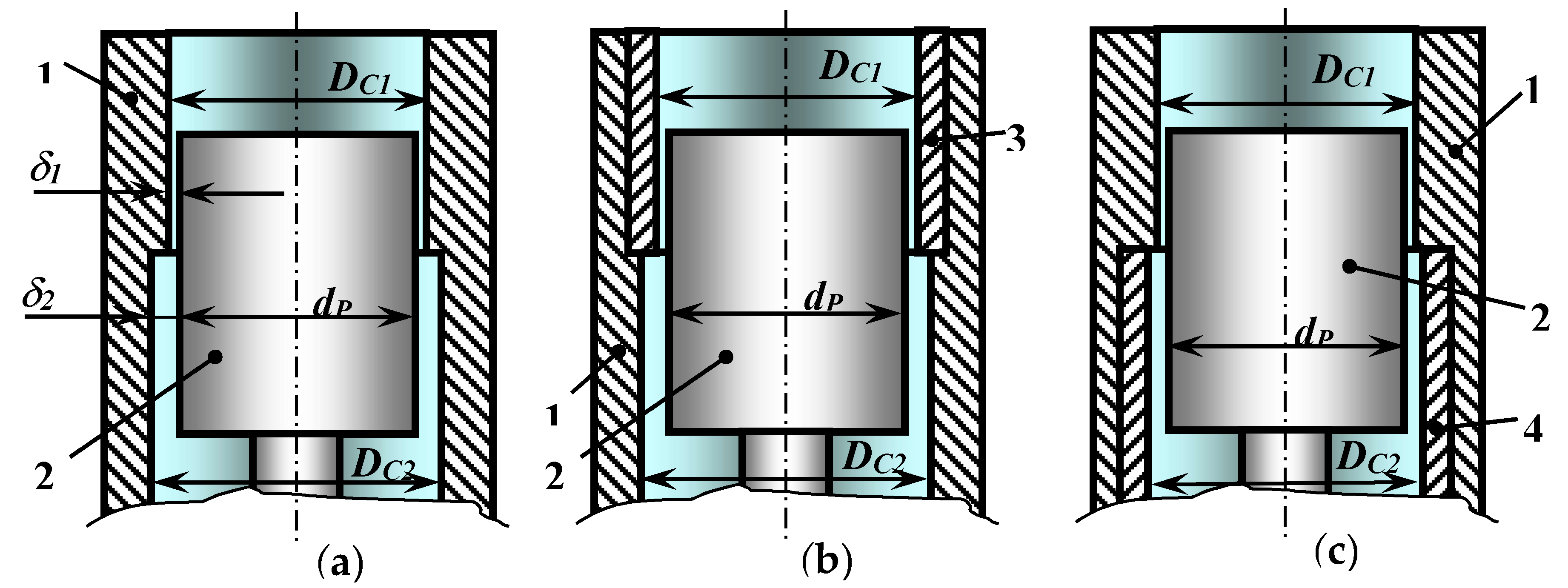
2. Analysis of the Main Types of Piston Seals Used in PHPM

The classic piston seal connecting the compressor and pump sections is a smooth gap of constant clearance along the length formed by the piston and cylinder [14,15], while the piston has a concentric or eccentric arrangement. When using a smooth gap seal, the flow rate of the fluid in the forward and reverse direction is the same. In accordance with the previously performed researches [16,17], the PHPM can operate in three modes, with the main mode being the priority flow of fluid from the pump fluid to the compressor. In this case, the piston seals must have different hydraulic resistance in the forward and return directions. When the fluid moves from the pump section to the compressor, the hydraulic resistance must be less than when the fluid moves from the compressor to the pump.

This effect can be achieved in various constructive ways. [18,19,20,21,22]. We consider the main ones.

There was considered a gap seal (see Figure 2), which has protrusions on the piston body and is profiled to provide difference in the flow rates of the fluid in the forward and return directions [19,23]. The multidimensional nonlinear optimization of the basic geometric parameters establishes their optimal values and achieve a ratio of fluid flow G_p/G_c = 1.3 ÷ 1.4, where G_p is mass flow of fluid per cycle from the pump section to the compressor; G_c is mass flow of fluid per cycle from the compressor section to the pump. It should be noted that this ratio is small and it was necessary to increase it. This was achieved in subsequent studies.

A piston seal of a step-type form has been studied (see Figure 3). It consists of a gap with small δ₁ and large δ₂ clearances and it works as follows: when the piston moves from the top dead center (TDC) to the bottom dead center (BDC), the fluid is compressed and injected in the pump section and the gas expands and sucks in the compressor. Piston seal length with low clearance 1 decreases and with a large clearance 2 increases, and in general, the hydraulic resistance of the gap along the piston is constantly decreasing. During the piston stroke from BDC to TDC, gas compression and injection are in the compressor section, and expansion and absorption are in the pump section. The fluid from the compressor section through the gap seal enters the pump section. It should be noted that in this case, the hydraulic resistance of the gap increases due to the fact that the length of the gap with a small clearance δ₁ increases, and the length of the gap with a large clearance δ₂ decreases. Thus, for a given type of gap seal, the G_p/G_c value can be 4 ÷ 5. Even better results can be expected from a gap seal, which does not change the length along the piston, but the clearance [22]. However, studies of the PHPM with such gap seals were not carried out.

Thus, to study the fluid flow in a piston seal, it is advisable to consider two types of gap seals: a smooth gap with a constant clearance and a gap with a stepwise change in the clearance.

3. Theoretical Research

The analysis of theoretical and experimental studies of PHPM is to determine the most characteristic values of geometric and operational parameters:

• The suction pressure in the compressor and pump section was always assumed to be the same and equal to 0.1 MPa.
• The discharge pressure in the compressor and pump sections was in the range from 0.3 to 1.0 MPa. To conduct theoretical research and to compare the flow rates of fluid in the forward and return directions, we assume that P_dp = P_dc = 1 MPa (where P_dp is discharge pressure in the pump section; P_dc discharge pressure in the compressor section).
• The piston diameter of the studied PHPM was from 0.04 to 0.06 m. We assume that the piston diameter is 0.04 m in these studies.
• The length of the piston actually determines the length of the piston seal. It varies in different PHPM designs. We assume that the length of the piston is 0.04 m in these studies.
• The magnitude of the radial clearance is one of the most important parameters. It was shown in [24] that the rational values for a smooth gap seal for a crosshead free PHPM are (20 ÷ 30) μm. It was proved in [25] that rational clearances δ₁ and δ₂ are (30 ÷ 55) μm and (80 ÷ 110) μm for a step-type piston seal in a crosshead PHPM respectively. In this paper, we assume that δ₁ is 25 μm, and δ₂ is 50 μm, i.e., those values are close to rational.

3.1. Laminar Fluid Flow

For the steady flow of incompressible viscous fluid, we obtain the equations for the distribution of fluid in the annular gap, the average velocity and flow rate for the fixed and moving walls with a concentric and eccentric arrangement of the piston from the equilibrium of the acting forces [24].

The fluid flow rate without taking into account the frictional motion and for the concentric arrangement of the piston in the cylinder is determined as:

$$Q=\frac{\pi d{\delta }^3\Delta p}{12\mu l_n}$$

(1)

where d is the cylinder diameter; µ is dynamic fluid viscosity; Δp is piston differential pressure; δ is radial clearance. The average velocity is determined as:

$$V=\frac{{\delta }^2\Delta p}{12\mu l_n}$$

(2)

Reynolds number is defined as:

$$Re=\frac{V\delta }{\mu /\rho }$$

(3)

It should be noted that the critical number Re_cr the laminar flow mode is carried out in a smooth gap is within 1000 ÷ 1200.

Using Equations (2) and (3), the value of the radial clearance the laminar mode of fluid flow will be observed is defined as:

$${\delta }_{cr}\le \sqrt[3]{\frac{12{Re}_{ĸp}{\mu }^2{\ell }_n}{\rho \Delta p}}$$

(4)

For accepted values ${\ell }_n$ and Δp, and also considering that the studied fluid is water, and at T = 293 K ρ = 998.2 kg/m³ and μ = 10⁻² Pa s, as well as considering that Re_cr = 1000, we obtain that δ_cr ≤ 80.5 μm, laminar mode will be realized with radial clearance values up to 80.5 μm. To calculate the step-type gap seal in [25], the equality of the combined costs is used Q₁ and Q₂ through its narrow and wide parts, while it is believed that the local resistance due to the step-type change in the radial clearance is negligible.

Using equality of expenses Q₁ and Q₂, pressure P3 is written in the section of step-type clearance as

$$P_3=\frac{\left(\frac{{\delta }_1^3}{{\ell }_1}\right)P_{ĸ}+\left(\frac{{\delta }_2^3}{{\ell }_2}\right)P_p}{\frac{{\delta }_1^3}{{\ell }_1}+\frac{{\delta }_2^3}{{\ell }_2}}$$

(5)

where ${\ell }_1$ and ${\ell }_2$ are seal lengths with clearance δ1 and δ2.

The fluid flow rate in this case is determined as:

$$Q_1=Q_2=\frac{\pi d{\delta }_1^3}{12\mu {\ell }_1}\left(P_H-P_3\right)=\frac{\pi d{\delta }_2^3\left(P_3-P_p\right)}{12\mu {\ell }_2}$$

(6)

Reynolds number is determined as:

$${Re}_1=\frac{{\delta }_1^3\left(P_c-P_3\right)\rho }{12{\mu }^2{\ell }_1}$$

(7)

$${Re}_2=\frac{{\delta }_2^3\left(P_3-P_p\right)\rho }{12{\mu }^2{\ell }_2}$$

(8)

Values ${\ell }_1$ and ${\ell }_2$ are interconnected by the following equality ${\ell }_1+{\ell }_2={\ell }_n$, where ${\ell }_n$ is the piston length.

3.2. Turbulent Fluid Flow

In general case to describe the unsteady flow of viscous compressible fluid, the following system of equations can be used, including the continuity equation, the equation of motion in the form of the Navier-Stokes equation, the energy conservation equation:

$$\frac{\partial \rho }{\partial t}+div\left(\rho V\right)=0$$

(9)

$$\rho \frac{\partial V}{\partial t}+\rho \left(V\cdot \nabla \right)V=-grad\left(p\right)+Div\left(\tau \right)$$

(10)

$$\frac{\partial }{\partial t}\left(\rho H\right)+\nabla \cdot \left(\rho VH\right)-\nabla \cdot \left(\frac{\lambda }{c_p}\nabla \left(h\right)\right)=\frac{\partial p}{\partial t}$$

(11)

The Navier-Stokes Equation (10) is Newton’s second law written for an infinitely small volume of fluid taking into account pressure forces and viscous friction forces. The left side of the equation includes local and convective acceleration, and the right side includes the forces of pressure and viscous friction, respectively grad(p) and $Div\left(\tau \right)$. Thermodynamic pressure p is determined as $p=\frac{1}{3}\left({\sigma }_{xx}+{\sigma }_{yy}+{\sigma }_{zz}\right)$, and the stress tensor τ is determined on the basis of the generalized Newton’s law of friction:

$$\tau =2\mu \dot{S}-\left(\frac{2}{3}\mu divV\right)E$$

(12)

where $E=\left(\begin{array}{ccc}1& 0& 0\\ 0& 1& 0\\ 0& 0& 1\end{array}\right)$; $S=\left(\begin{array}{ccc}\frac{\partial V_x}{\partial x}& \frac{1}{2}\left(\frac{\partial V_x}{\partial y}+\frac{\partial V_y}{\partial x}\right)& \frac{1}{2}\left(\frac{\partial V_x}{\partial z}+\frac{\partial V_z}{\partial x}\right)\\ \frac{1}{2}\left(\frac{\partial V_y}{\partial x}+\frac{\partial V_x}{\partial y}\right)& \frac{\partial V_y}{\partial y}& \frac{1}{2}\left(\frac{\partial V_y}{\partial z}+\frac{\partial V_z}{\partial y}\right)\\ \frac{1}{2}\left(\frac{\partial V_z}{\partial x}+\frac{\partial V_x}{\partial z}\right)& \frac{1}{2}\left(\frac{\partial V_z}{\partial y}+\frac{\partial V_y}{\partial z}\right)& \frac{\partial V_z}{\partial z}\end{array}\right)$;

Equation (11) is an energy conservation equation for an infinitely small volume, which is written taking into account the braking heat expressed in terms of the braking enthalpy H, which is associated with static enthalpy as follows: $H=h+{\left|V\right|}^2/2$, where $\left|V\right|$ is module of the velocity vector. To determine steady flow and incompressible fluid, taking into account constant temperature and, accordingly, constant thermophysical properties, the system of Equations (9)–(11) is transformed to the following form:

-

continuity equation:

$$\nabla \cdot V=0$$

(13)

-

Navier-Stokes equation:

$$\frac{\partial V}{\partial t}+\left(V\cdot \nabla \right)V=-\frac{1}{\rho }\nabla p+v{\nabla }^{2}V$$

(14)

where V is velocity vector.

The system of Equations (13) and (14) in the general case has no analytical solution and can be solved only numerically. Currently, three main methods are used to solve such systems of equations: the finite difference method, the finite volume method, and the finite element method. The finite volume method is most widely used due to the high computational stability. The idea of this method is to replace infinitely small volumes of fluid with volumes of finite sizes—cells. Equations (13) and (14) are written for each created cell, and the totality of all cells is called the computational grid. The theory of turbulent motions proves that turbulent fluid motions consist of many vortex formations having different geometric dimensions [26,27]. As a result, the cell sizes used for the numerical solution of the equations should be much smaller than the smallest turbulent formation. This condition determines the number of cells required to solve the problem. As a rule, these are tens and hundreds of millions of cells. The cell size of the computational grid is chosen much larger than the size of small-scale turbulent formations, as existing computers have insufficient performance to solve similar problems of fluid mechanics and it is necessary to reduce the number of cells [28]. In this way the number of cells in the grid can be significantly reduced. In this case, a certain number of turbulent structures will fall inside each of the grid cells, and, therefore, their characteristics cannot be determined on the basis of Equations (13) and (14), i.e., additional equations are required to calculate turbulence characteristics. To date, several empirical methods for calculating turbulence characteristics have been developed. Reynolds offered the most widely used method which consists in averaging variables.

The proposed averaging of Reynolds does not solve the problem, because it adds six additional unknowns to the system of equations, which are called “Reynolds stress”. Using the Boussinesq hypothesis simplifies significantly the Navier-Stokes Equation (14) and reduces the number of unknowns characterizing turbulence from six to one, turbulent viscosity. Turbulent viscosity is not a constant value, like molecular viscosity, but depends both on time and on spatial coordinates, and its value is calculated for each cell of the design string at each step of integration over time. The calculation of the turbulent viscosity is carried out using a semi-empirical model of turbulence. At present, a large number of such models have been created; however, two-parameter semi-empirical turbulence models are most widely used. This is due to the fact that these models are the most stable, although they are less accurate than a number of other models.

The analysis of existing turbulence models revealed three models; their use is expedient for calculating the flow in a gap seal of a piston hybrid power machine.

3.3. Turbulence Model $k-\epsilon$

Turbulence model $k-\epsilon$ is one of the most widely used models of turbulence and it consists of two equations: kinetic energy of turbulence k and dissipation of kinetic energy $\epsilon$. The main idea underlying this model is to describe the processes of nucleation, transfer, and dissipation of turbulence. To implement this idea, the following differential transport equations k and $\epsilon$ were used:

$$\frac{\partial }{\partial t}\left(pk\right)+div\left(\rho Vk\right)=div\left(\left(\mu +\frac{{\mu }_t}{{\sigma }_k}\right)grad\left(k\right)\right)+P_k-\rho \epsilon +P_{kb}$$

(15)

$$\frac{\partial }{\partial t}\left(p\epsilon \right)+div\left(\rho V\epsilon \right)=div\left(\left(\mu +\frac{{\mu }_t}{{\sigma }_{\epsilon }}\right)grad\left(\epsilon \right)\right)+\frac{\epsilon }{k}\left(C{\epsilon }_{\epsilon 1}{P}_k-C_{\epsilon 2}\rho \epsilon +C_{\epsilon 1}{P}_{\epsilon b}\right)$$

(16)

In these equations k is kinetic energy of turbulence; $\epsilon$ is turbulence energy dissipation; P_k is generation (generation) of turbulence energy, which is calculated by the following dependence for an incompressible fluid:

$$P_k={\mu }_t\left(\frac{\partial V_i}{\partial V_j}+\frac{\partial V_j}{\partial x_i}\right)\frac{\partial V_i}{\partial x_j}$$

(17)

where $P_{kb}$ and $P_{\epsilon b}$ are terms that take into account the effects of gravity which are usually neglected.

Joint solution of Equations (15) and (16) is to calculate the distribution k and $\epsilon$ over the computational domain at a given point in time, then the value of turbulent viscosity for each computational cell is calculated. A number of empirical constants are used in the turbulence model $k-\epsilon$, its value is determined by calibrating the model according to a series of field experiments. References prove that the model $k-\epsilon$ calibrated for developed turbulent fluid flows and can mainly be used to describe the free flow of fluid at a sufficient distance from the solid walls.

The main disadvantages of the model include:

• Instability of work with flows having a large pressure gradient and a powerful degree of turbulence.
• This model gives an overestimated value of kinetic energy at high speeds of movement of the working fluid.

3.4. Turbulence Model $k-\omega$

$k-\omega$ model was developed to eliminate $k-\epsilon$ model flaws. It was developed to calculate fluid motion taking into account the presence of solid walls. Turbulent viscosity in the model $k-\epsilon$ is determined as follows:

$$v_t=\frac{k}{\omega }$$

(18)

It should be noted that the $k-\omega$ model equation has a similar physical meaning and structure with equations $k-\epsilon$ models and differ in closure constants and terms describing the generation and dissipation of variables k, $\omega$ and $\epsilon$.

Despite all the positive properties, $k-\omega$ model of turbulence, it is unacceptable in a number of cases, for example, when describing the developed turbulent motion away from solid walls and having direct contact with them. In this case, high accuracy is required for calculating the turbulence characteristics both near and far from solid walls. An example of such cases is the problem of separation of the boundary layer from a solid wall. In these cases when there is separation of the boundary layer, $k-\epsilon$ turbulence models are poorly described as well as $k-\omega$ models.

3.5. Turbulence Models SST

Menter developed the Shear StressTransport (SST) turbulence model that includes both $k-\epsilon$ and $k-\omega$ turbulence models to increase the accuracy of the description of turbulent flows in which there is a probability of boundary layer separation. This became possible due to the high similarity of these models’ equations. With a certain combination of empirical constants SST turbulence model can be reduced to $k-\epsilon$ model or to $k-\omega$ model.

SST turbulence model includes two differential equations describing the transfer of turbulence energy k and the intensity of its dissipation $\omega$. The model uses two functions F₁ and F₂ – these are the transition functions between $k-\epsilon$ and $k-\omega$ turbulence models. Far from a solid wall, these functions turn into 0, while the SST turbulence model comes down to a standard model $k-\epsilon$. Function F₁ and F₂ tend to 1 inside the boundary layer, which corresponds $k-\omega$ model. A smooth transition from one model to another takes place in the space between the boundary layer and the developed turbulence model. All empirical constants of SST turbulence models are calculated by recalculating the corresponding constants $k-\epsilon$ and $k-\omega$ models using the function F1 followed by addiction:

$$a=a_1{F}_1+a_2\left(1-F_1\right)$$

(19)

where a is SST constant of turbulence model; a₁ and a₂ are constant $k-\epsilon$ and $k-\omega$ models respectively.

For the successful application of the SST turbulence model, it is necessary to choose the right cell size directly near the solid wall. The SST model does not use the transport equation for turbulent shear stresses, but calculates the shear stresses themselves using the Boussinesq hypothesis based on the application of the concept of turbulent viscosity. The value of turbulent viscosity is determined similarly to the model $k-\omega$, but with the introduction of a limiter. This representation of turbulent viscosity is to solve problems with the appearance of separated flow flows with changes in the sign of the pressure gradient near the wall.

There are many other turbulence models, in particular, a group of RSM models based on the additional tensor in the Reynolds equations which includes the so-called Reynolds stresses or turbulent stresses. These are RSM, Explicit Algebraic Reynolds Stress Model (EARSM) and other models. The main advantage of such models is the inclusion of turbulence anisotropy which takes into account the turbulence characteristics in different directions of space. The disadvantages include a large number of calibration empirical coefficients which significantly reduce the versatility of this model and the inability to apply it without changing the coefficients to other turbulent flows. The analysis of references, based on material costs, decision time and quality of the results allowed focusing on three main models: $k-\epsilon$, SST and RSM.

It should be noted that a complex of experimental studies was carried out in [2] to determine the flow rate of liquid through smooth slots in a turbulent flow mode, its results were processed and fluid flow formulas were obtained for concentric and eccentric arrangement of the piston.

For the concentric piston arrangement in the cylinder we have:

$$Q=0.424\pi d\nu {\left(\frac{{\delta }^3\Delta p}{{\ell }_n\rho {\nu }^2}\right)}^{0.813}$$

(20)

where $\nu =\mu /\rho$ is kinematic viscosity.

For a step-type seal using the equality of volumetric flow rates in the narrow and wide parts of the piston seal we obtain the following Equation for pressure p₃:

$$p_3=\frac{\frac{{\delta }_1^3{\ell }_2}{{\delta }_2^3{\ell }_1}\left(p_1+p_2\right)}{\left(1+\frac{{\delta }_1^3{\ell }_2}{{\ell }_1{\delta }_2^3}\right)}$$

(21)

and flow:

$$Q=Q_1=Q_2=0.424\pi d\nu {\left[\frac{{\delta }_2\left(p_3-p_2\right)}{{\ell }_2\rho {\nu }^2}\right]}^{0.813}$$

(22)

Using Equations (20) and (22), we can evaluate the reliability of the turbulence models considered above.

4. Data Analysis

A numerical experiment will be conducted on the applicability of the turbulence models discussed above, as well as the Laminar model, for calculating smooth and step-type gap seals in laminar and turbulent modes in a piston hybrid power machine. We calculate the flows in gap seals using the ANSYS CFX application software package which includes turbulence model data.

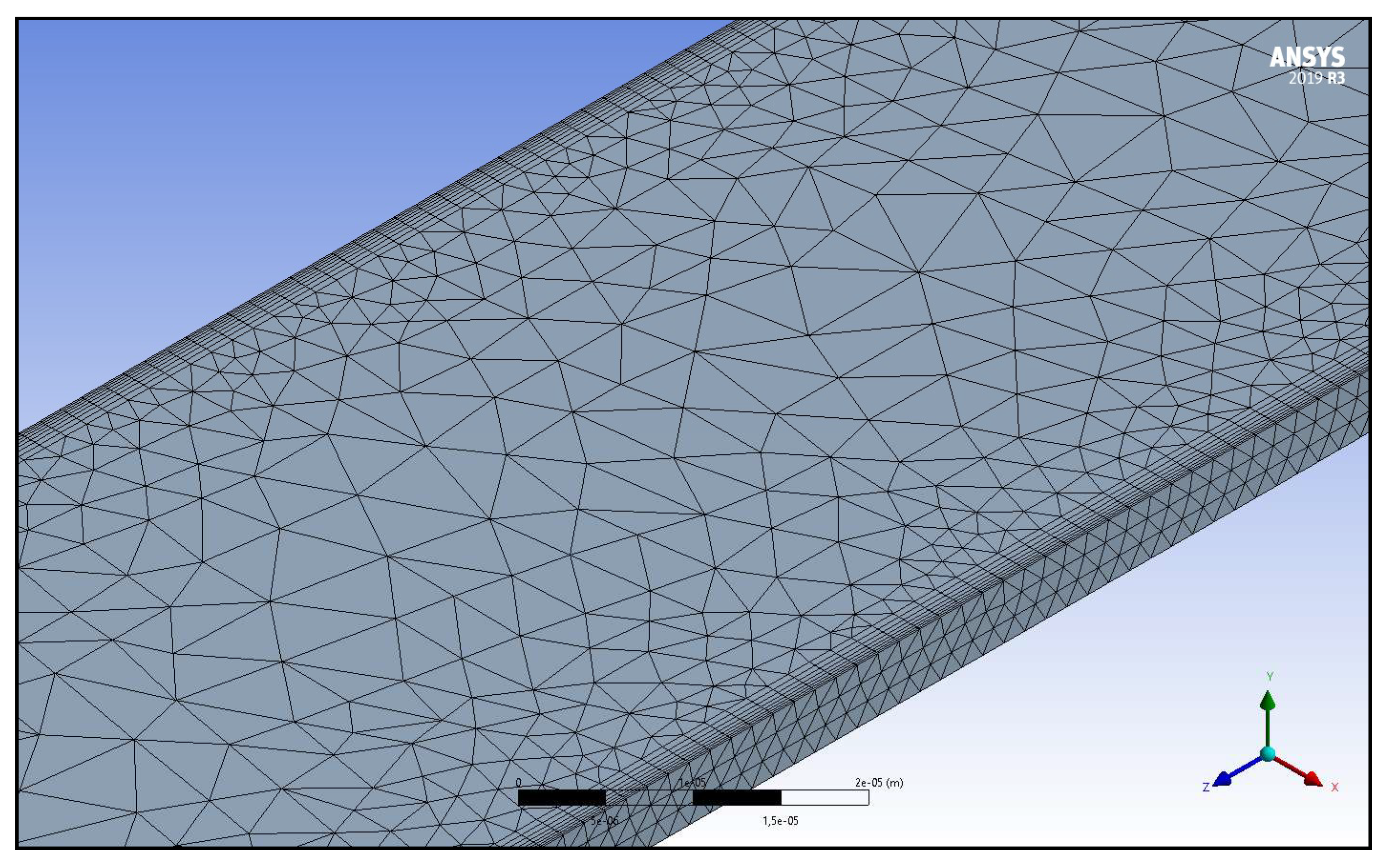
4.1. Implementation Features

Assuming that the problem under consideration is axisymmetric, a gap seal segment with an angular width was considered 0.01⁰ to reduce the calculation time and reduce the number of cells. When determining the total flow rate in a gap seal, the flow rate determined in this segment is multiplied by 36,000.

The segments of gap seals with constructed meshes are shown in Figure 4 and Figure 5. The construction of the finite elements was carried out automatically in a smooth gap seal, and it was carried out automatically with manual correction in a step-type gap seal at the points of rotation on 90⁰.

We conduct a sequential review of gap seals.

4.2. Smooth Gap Seal

4.2.1. Laminar Flow

Diagrams of velocity distribution along the cross section of the gap are presented in Figure 6.

Analyzing the presented data, we have the following conclusions:

• The velocity distribution diagrams of the RSM and SST turbulence models are closest to the theoretical velocity distribution determined in accordance with [4,5]. The discrepancy in determining the maximum speed between them is approximately equal to 1 m/s, i.e., 14.2%.
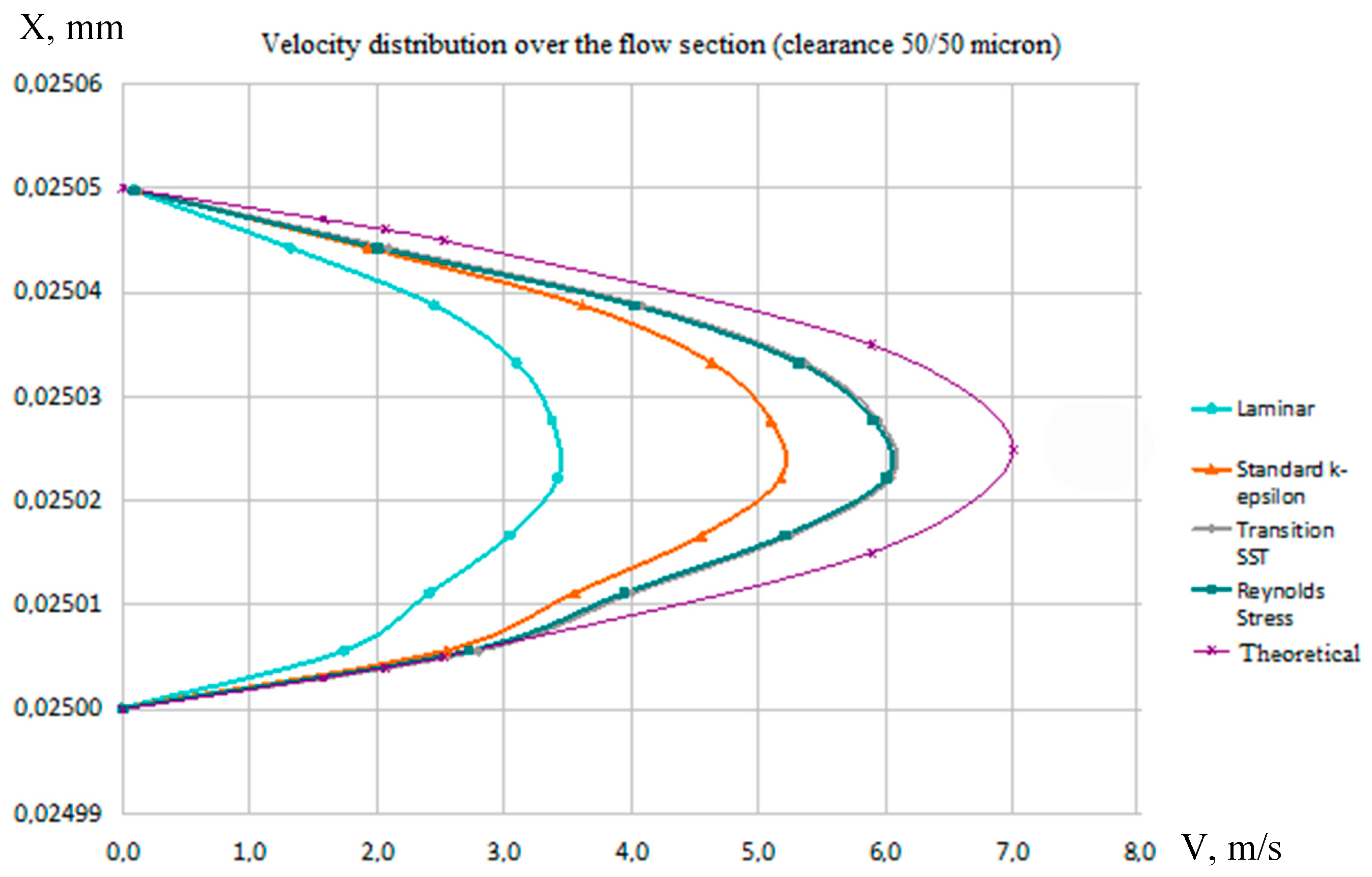
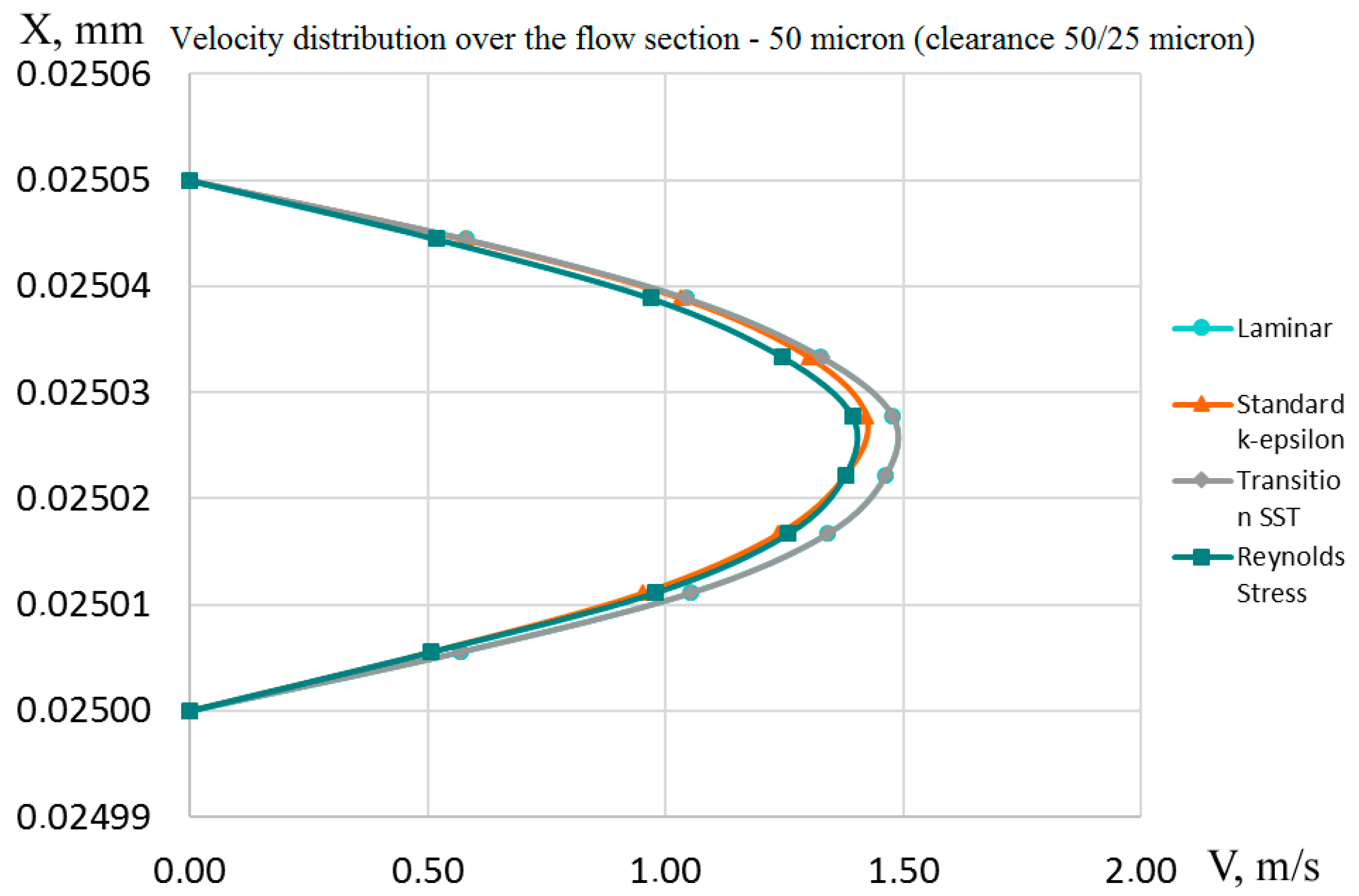
• Speed distribution by model $k-\epsilon$ is significantly better than laminar model. The discrepancy in determining the maximum speed model $k-\epsilon$ is 2 m/s, i.e., 28.4%. The discrepancy in determining the maximum speed of the laminar model is 3.5 m/s, i.e., 50%.

Table 1. Average fluid velocities in the gap and Reynolds numbers determined by different flow models for the laminar modes with a gap seal 50/50 μm.

Turbulence Models	The Size of the Gap Seal 50/50, Microns
	Vav, m/s	Re
Laminar	2.424	120.475
Standard k-epsilon (input/output)	3.707	184.25
Transition SST (input/output)	4.234	210.42
Reynolds Stress (input/output)	4.174	207.433
Formula Consumption: $Q=\frac{\pi d{\delta }^3\Delta p}{12\mu l_n}$	3.74	185.887

presents the average fluid velocities in the gap and the Reynolds numbers determined by different flow models.

The presented results lead to the following conclusions:

• The Reynolds numbers determined by different models are in the range from 120 to 210, which allows supposing that there is a laminar flow mode in the gap seal. It should be noted that this conclusion could be made from the previously considered results (velocity diagrams).
• The maximum average velocities of 4.234 and 4.174 m/s are observed using the SST and RSM turbulence models. These average velocities exceed significantly (almost by 0.5 m/s) the average velocities determined by calculation for the laminar fluid flow in the gap [3], and according to the turbulence model $k-\epsilon$.
• The lowest average velocity of 2.404 m/s is shown by the laminar fluid flow model which is almost 1.3 m/s less than the theoretically calculated.
• $k-\epsilon$ model shows the closest to theoretically calculated values by the definition of average velocity. The discrepancy in determining the average velocity, compared with the theoretically determined one, is 0.033 m/s or 0.88%, i.e., less than 1%. The discrepancy in the definition of average velocities is equivalent to the discrepancy in the definition of volumetric costs presented in

  Table 2. Volume flow through a gap defined by different flow models for different sizes of gap seals for laminar flow.

  Turbulence Models	The Size of the Gap Seal (Input Flow/Output Flow), Microns
  	25/50	50/25	50/50
  Laminar	0.008070 kg/s	0.008036 kg/s	0.018989 kg/s
  Standard k-epsilon (input/output)	0.007822 kg/s	0.007304 kg/s	0.029041 kg/s
  Transition SST (input/output)	0.008060 kg/s	0.008031 kg/s	0.033166 kg/s
  Reynolds Stress (input/output)	0.007428 kg/s	0.007478 kg/s	0.032695 kg/s
  Formula Consumption: $Q=\frac{\pi d{\delta }^3\Delta p}{12\mu l_n}$	−0.006507 kg/s	−0.006507 kg/s	0.029299 kg/s

  .

Thus, summarizing the analysis of the laminar flow in the smooth gap of the PHPM, we can conclude that it is preferable to use SST and RSM to determine the maximum values of velocities, and the $k-\epsilon$ model to determine average velocities and costs.

4.2.2. Turbulent Flow

The turbulent flow, in contrast to the laminar flow, is characterized by the presence of vortices and intensive mixing of the fluid in the transverse direction. To obtain a turbulent flow in the gap seal while maintaining the differential pressure and length of the gap seal, it is necessary to increase the gap in the gap seal. In accordance with previous calculations, the gap should be more than 80.5 microns. We take 100 μm for accuracy, because if the gap is more than 100 μm, then the operation of the gap seal becomes ineffective and, accordingly, the study is not of scientific interest.

The velocity distribution when using different flow models is close to the laminar one, then the laminar model was considered together with turbulent models. Figure 7 shows cross-sectional velocity plots for the models under consideration.

From the presented data, we can draw the following conclusions:

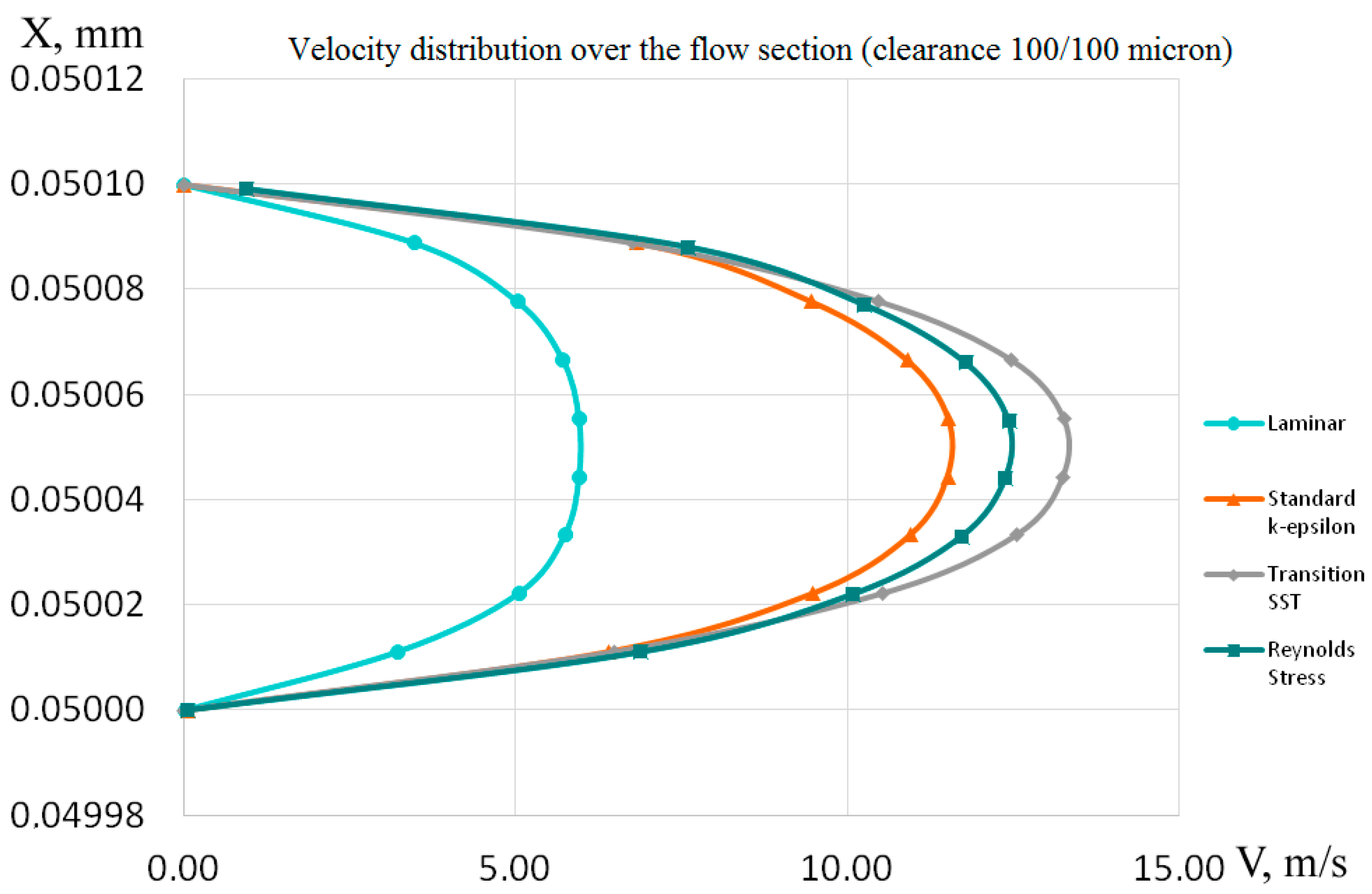
• The maximum values of velocities are almost doubled and amount to (12 ÷ 13) m/s. The highest maximum velocity is observed in the RSM model. The differences between the maximum values of the fluid flow rate, determined by the RSM and SST models, are about 1 m/s, while they practically coincided in laminar flow.
• The lowest maximum speed is observed when using the laminar model. It is about 5 m/s, which is more than two times less than the maximum speed obtained by the RSM model.

Table 3. Average fluid velocities in the gap and Reynolds numbers determined by different flow models for the turbulent mode with a gap seal size of 100/100 μm.

Turbulence Models	Sizes of Slotted Seals 100/100, Microns
	Vav, m/s	Re
Laminar	4.658079432	463.0298
Standard k-epsilon (input/output)	8.889252625	883.6235
Transition SST (input/output)	9.853676103	979.4907
Reynolds Stress (input/output)	9.510253468	945.3532
Formula Consumption: $Q=0.424\pi d\nu {\left(\frac{{\delta }^3\Delta p}{{\ell }_n\rho {\nu }^2}\right)}^{0.813}$	11.67878943	1160.913

presents the average velocities and Reynolds numbers for different models of fluid flow determined by the results of experimental studies [2].

Analyzing the presented results, we have:

• The average velocities calculated from the considered flow models are significantly less than the average velocity determined experimentally. The average velocity determined by the SST model is the closest value.
  However, the discrepancy is 1.83 m/s, which is 15.67%.
• The lowest average velocity of 4.66 m/s is shown by the laminar model, which is less than two times less than the velocity determined experimentally.
• It should be noted that the Re number determined by the average velocity for all turbulence models is less than 1000. Only the Re number determined by the average velocity determined on the basis of experimental data is more critical than the number Re_cr (Re_cr = 1000) and is 1160. This suggests that we are generally in the transition area between the laminar and turbulent flow modes.

The volumetric flow rate of the fluid (see

Table 4. Volume flow through a gap defined by different flow models for different sizes of gap seals for turbulent flow conditions.

Turbulence Models	The Size of the Gap Seal (Input Flow/Output Flow), Microns
	50/100	100/50	100/100
Laminar	0.060259 kg/s	0.059219 kg/s	0.073149 kg/s
Standard k-epsilon (input/output)	0.044047 kg/s	0.045038 kg/s	0.139594 kg/s
Transition SST (input/output)	0.060051 kg/s	0.059162 kg/s	0.154739 kg/s
Reynolds Stress (input/output)	0.056449 kg/s	0.057229 kg/s	0.149346 kg/s
Formula Consumption: $Q=0.424\pi d\nu {\left(\frac{{\delta }^3\Delta p}{{\ell }_n\rho {\nu }^2}\right)}^{0.813}$	0.053999 kg/s	0.053999 kg/s	0.1834 kg/s

), determined by the SST turbulence model, as well as the average velocity, is closest to the flow rate determined from experimental studies.

Summing up the study of turbulent flow in a smooth gap, we can conclude that the results obtained using the SST and RSM turbulence models are closest to the experimental results and, therefore, their application in this case is preferable.

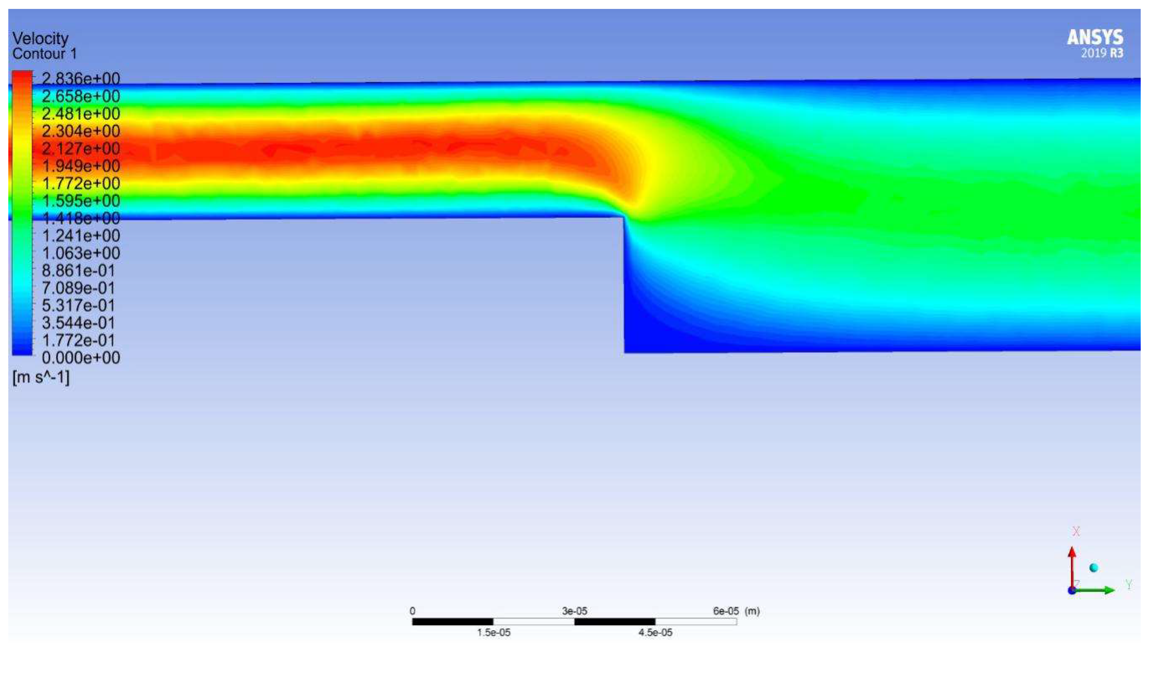
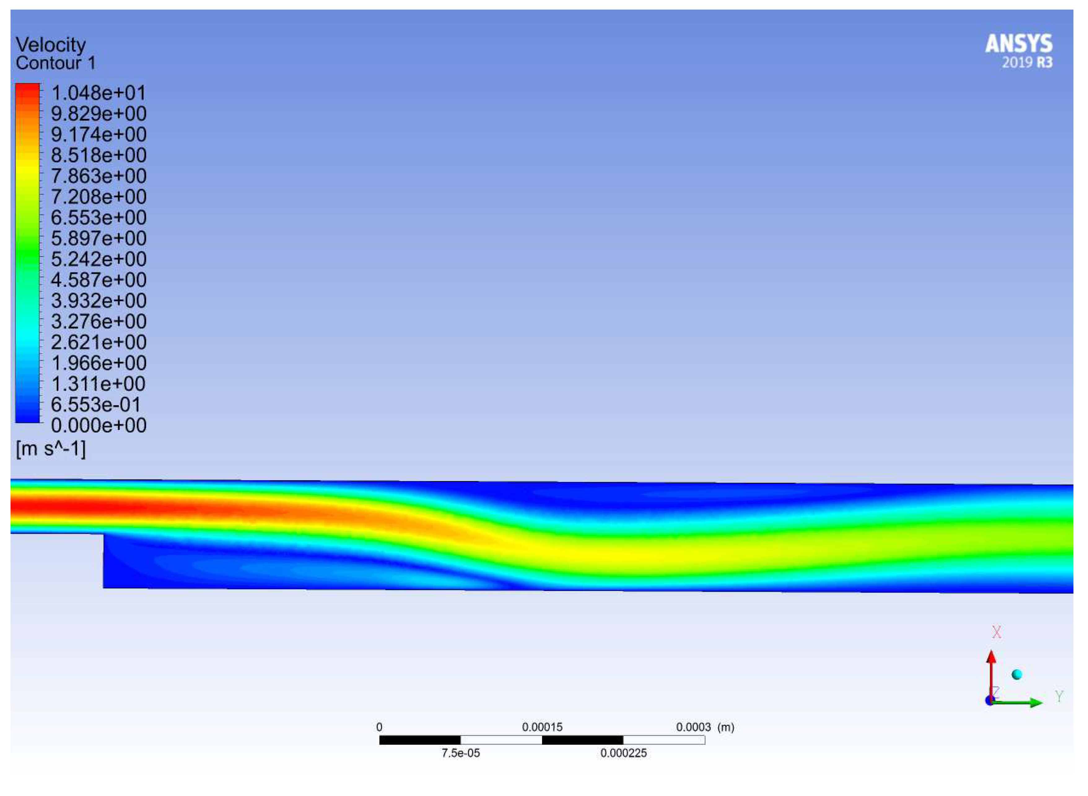
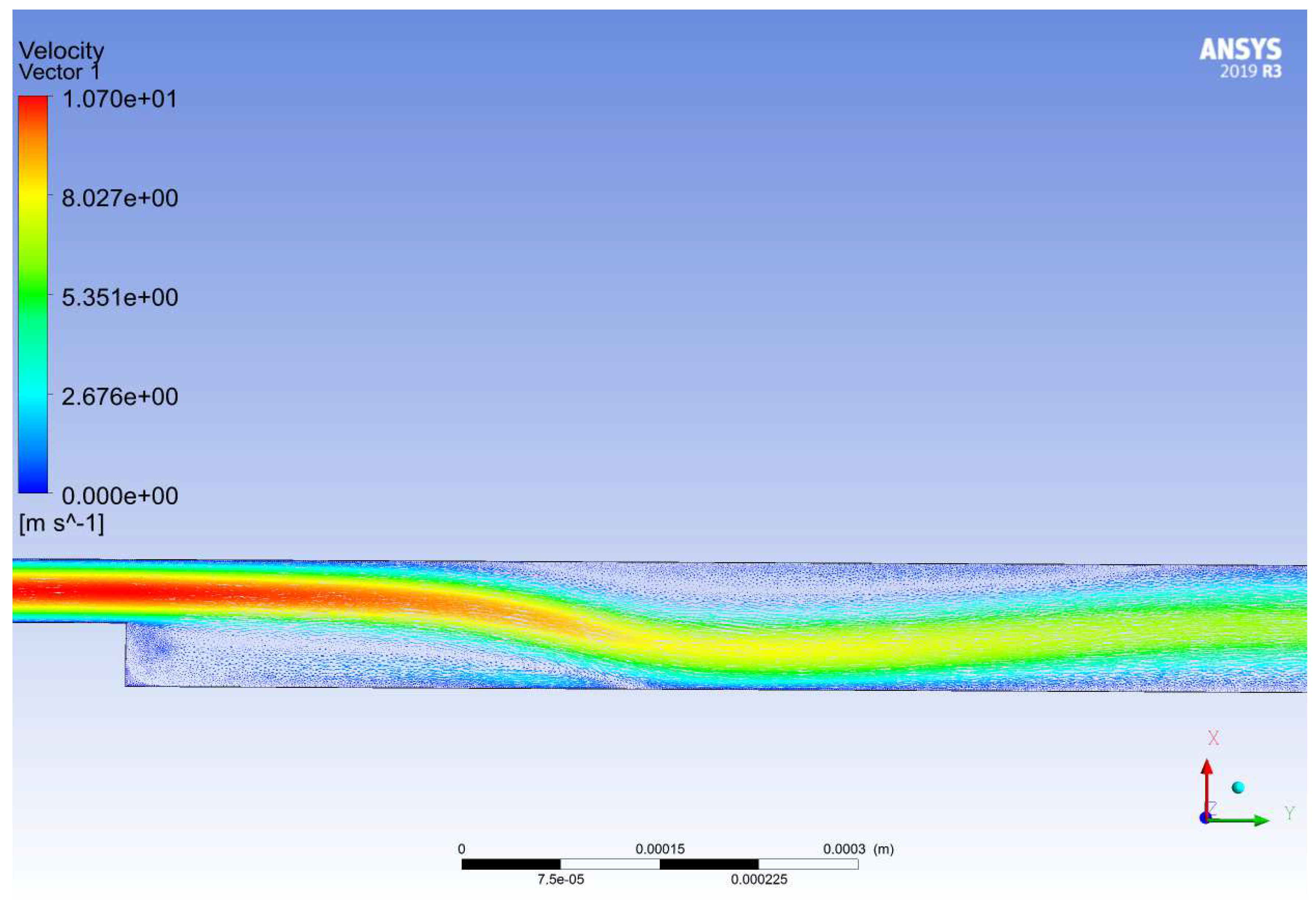
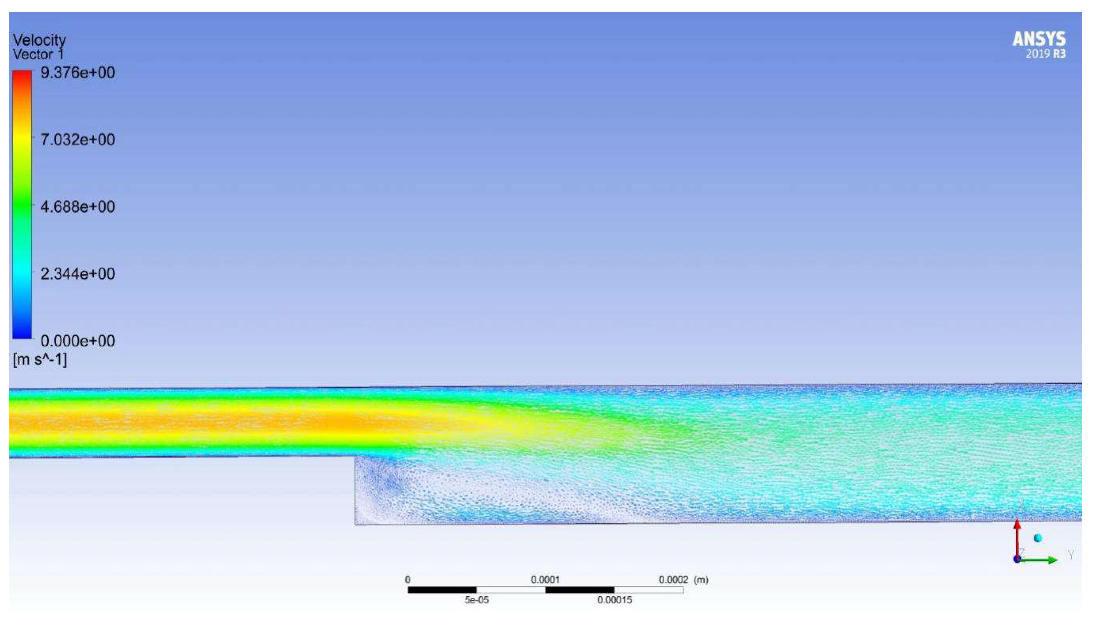
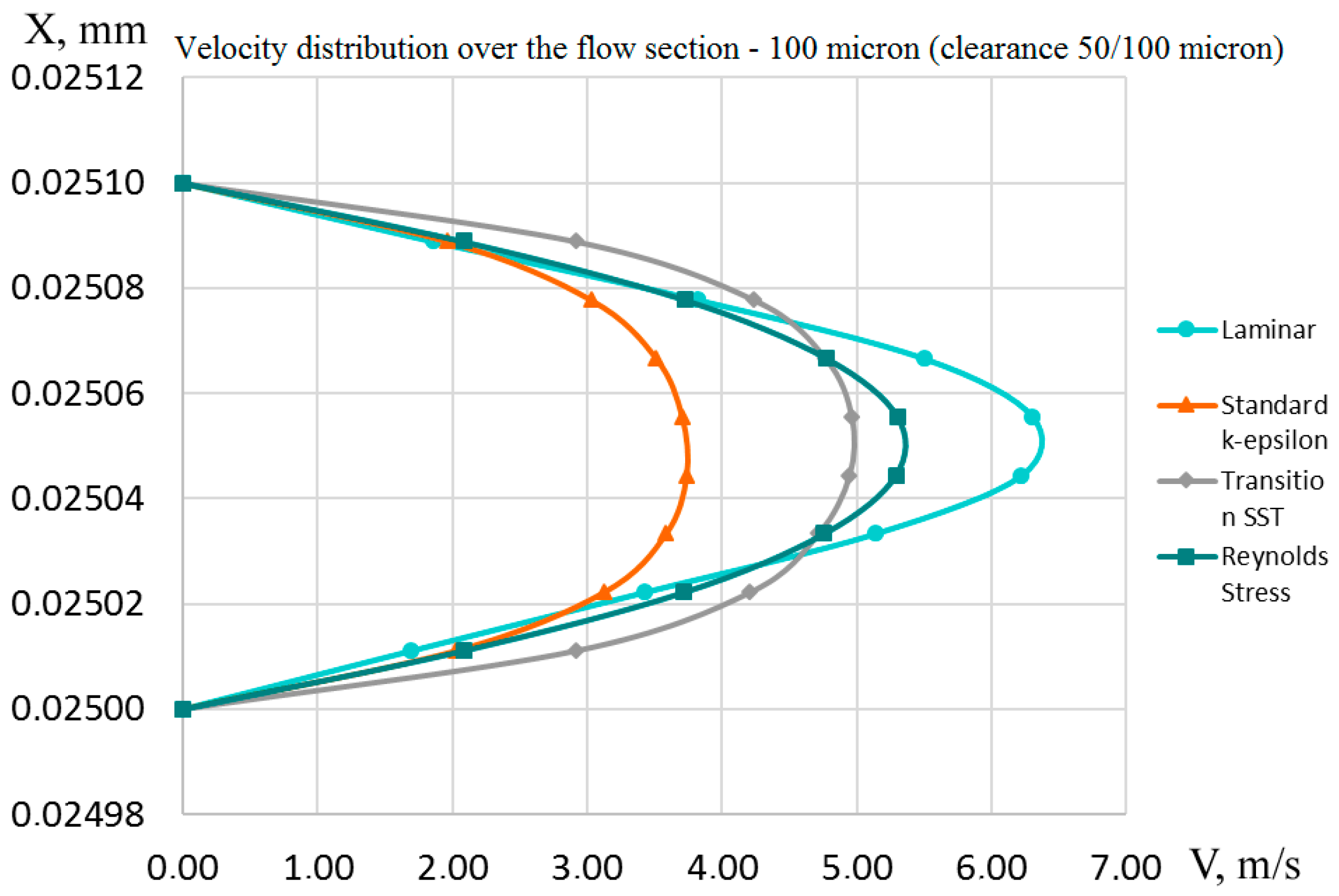
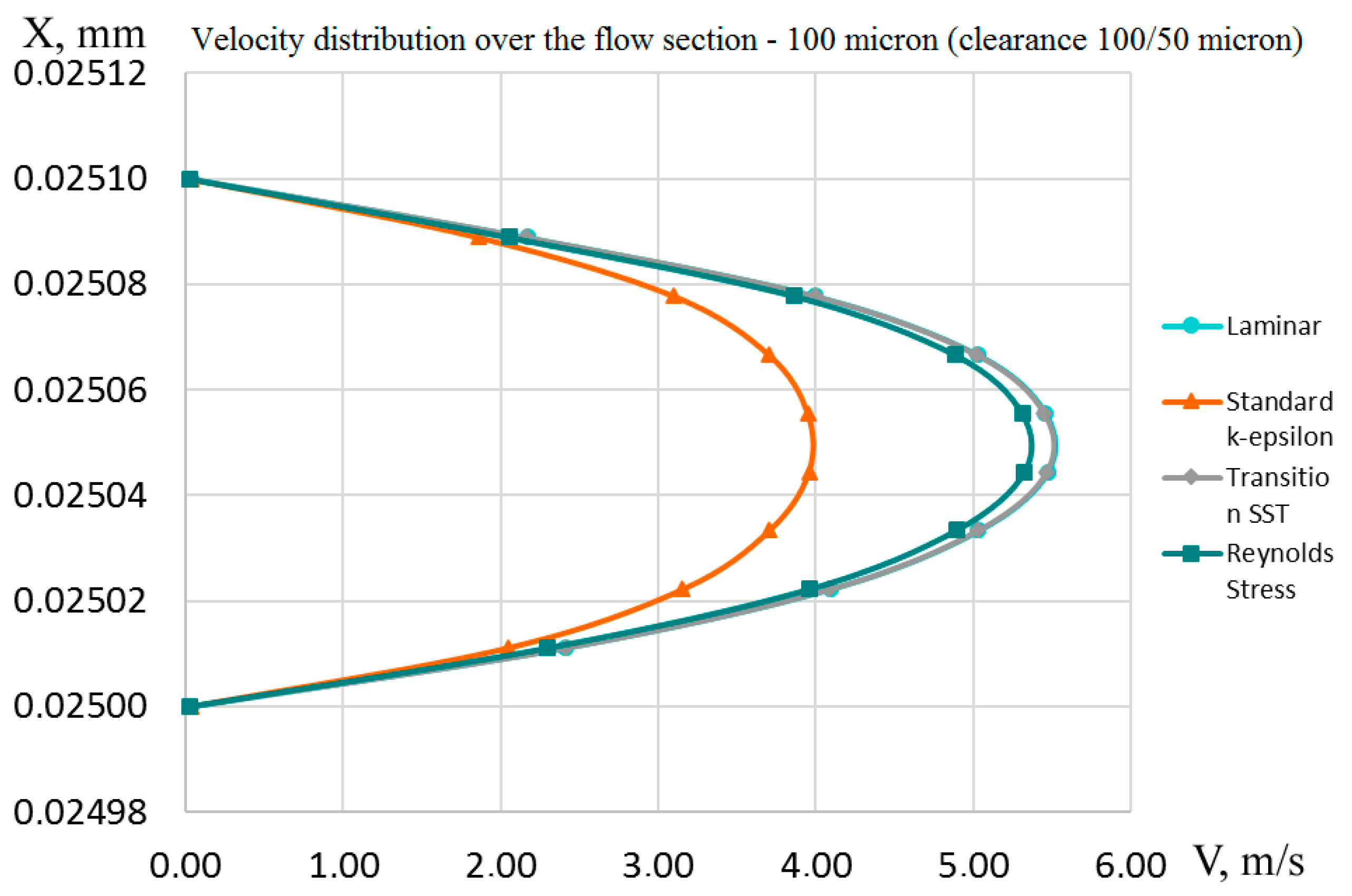
4.3. Step-Type Gap Seal

4.3.1. Laminar Flow

There is considered the flow of a viscous fluid in a step-type gap seal with a change in the gap from 25 to 50 μm in the forward and reverse directions. The step is organized from the left border of the gap seal at a distance ℓ_cm = ℓ_yn/2.0 = 20 MM, i.e. half its length. Reducing the gap by half the length of the gap seal leads to a decrease in the overall average gap in the gap seal, which leads to a decrease in the velocity and flow rate of the fluid in the gap seal. During the analysis, we will consider the diagrams of instantaneous velocities and the average fluid velocity in two sections: with a gap of 25 μm and with a gap of 50 μm.

Figure 8 shows the velocity plots in the cross section with a gap of 50 μm obtained using various flow models.

The maximum velocity in a gap seal of about 1.5 m/s is achieved using the SST and laminar turbulence models. The maximum velocities in the remaining flow models are approximately equal and less by about 0.2 m/s.

Table 5. Values of average velocities and Reynolds numbers for fluid flow in a step-type gap seals in the forward direction determined by different flow models.

Turbulence Models	The Size of the Gap Seal 50, Microns
	Vav, m/s	Re
Laminar	1.030141717	102.399773
Standard k-epsilon (input/output)	0.998484326	99.25291509
Transition SST (input/output)	1.028865209	102.2728836
Reynolds Stress (input/output)	0.948189922	94.2534714
Formula Consumption: $Q_1=Q_2=\frac{\pi d{\delta }_1^3}{12\mu {\ell }_1}\left(\Delta p\right)=\frac{\pi d{\delta }_2^3\left(\Delta p\right)}{12\mu {\ell }_2}$	0.830623563	82.56695455

presents the mean velocities and Reynolds numbers for fluid flow in a gap seal. The results presented in the Table 5 prove that the minimum discrepancy in average velocity and, accordingly, in flow rate between theoretically calculated by formula [2] $\upsilon =\frac{\Delta p}{2\mu l_n}\left(\frac{{\delta }^2}{4}-y^2\right)$ and model, provides the RSM turbulence model, then $k-\epsilon$ model and the SST model. The greatest discrepancy is observed when using the laminar model.

Diagrams of the velocity distribution in the same section are presented in Figure 9, but when the fluid flows in the opposite direction for different turbulence models. When comparing the diagrams of the velocities of the forward and reverse flows, we can conclude that these diagrams qualitatively and quantitatively coincide.

In general, it is known from the theory of hydraulic resistances that hydraulic losses during sudden expansion exceed hydraulic losses during sudden narrowing [4,5].

A significant parasitic vortex is formed with sudden expansion, which prevents the flow of the main stream. This phenomenon is well observed when using all flow models (for example, see Figure 10 and Figure 11). With a sudden narrowing, a parasitic vortex is also formed, but its size is much smaller and the localization is different. It is localized at a wall with a large gap near a sudden narrowing (see Figure 12 and Figure 13). Such a distribution of velocity vectors is characteristic of all flow models.

Table 6. Values of average velocities and Reynolds numbers during fluid flow in a step-type gap seals in the opposite direction determined by different flow models.

Turbulence Models	The Size of the Gap Seal 50, Microns
	Vav, m/s	Re
Laminar	1.025801591	101.9683
Standard k-epsilon (input/output)	0.932361227	92.68004
Transition SST (input/output)	1.025163337	101.9049
Reynolds Stress (input/output)	0.954572461	94.88792
Formula consumption: $Q_1=Q_2=\frac{\pi d{\delta }_1^3}{12\mu {\ell }_1}\left(\Delta p\right)=\frac{\pi d{\delta }_2^3\left(\Delta p\right)}{12\mu {\ell }_2}$	0.830623563	82.56695

presents the results of average velocities and Reynolds numbers for different models of fluid flow and the known theoretical dependence. The results presented in Table 6 on qualitative and quantitative characteristics practically correspond to the results presented in Table 5.

Comparing the results presented in Table 5 and Table 6, we have the following conclusions:

• Results on average velocity and fluid flow in a gap seal obtained by model $k-\epsilon$ are closest to the results obtained from known theoretical dependencies [2,4,5].
• The RSM model is the only turbulence model that has lower velocity and lower flow rate during sudden expansion (forward flow) compared to sudden compression (reverse flow).
• Taking into account that the RSM model describes correctly qualitatively and quantitatively the fluid flow in a step-type gap seals, the RSM model is to be used when calculating a step seal in laminar mode.

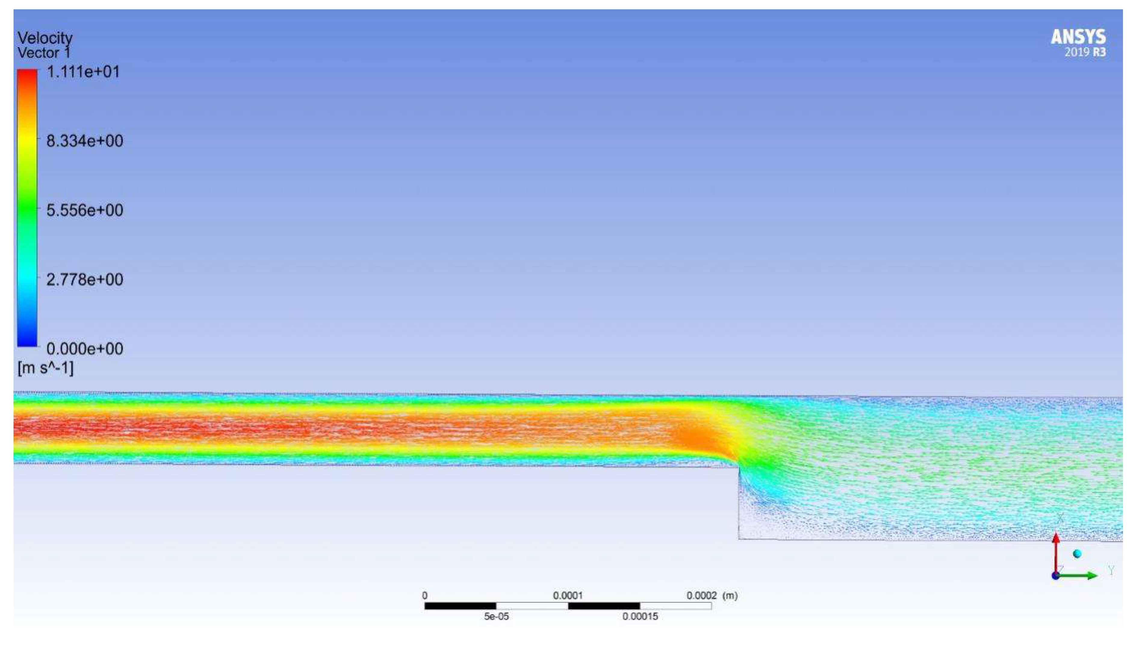
4.3.2. Turbulent Flow

The flow of a viscous fluid in a step-type gap seal is considered when the gap changes from 50 to 100 μm. In this case, a fluid flow is realized with a sudden expansion. Analyzing the patterns of the distribution of modules and velocity vectors, we can conclude that when using the laminar, SST, and RSM models, two areas with a stagnant-flow areas can be seen (see Figure 14 and Figure 15) and the curvature of the flow core.

When using $k-\epsilon$ model the distribution of moduli and velocity vectors has a different form (see Figure 16 and Figure 17). In this case, only one stagnant area is formed without curvature of the flow core.

For further analysis, we choose a section with a gap size of 100 μm. Figure 18 shows plots of the velocity distribution in the cross section of the gap seal.

The highest maximum speed (a little more than 6 m/s) is observed when using the laminar model, and the lowest maximum speed (about 3.5 m/s) is observed when using the $k-\epsilon$ turbulence model. This can also be seen in Figure 16. The RSM and SST flow models show approximately the same average values of maximum velocity and it is about 5 m/s.

Analyzing the values of average velocities in a gap seal obtained using different models of viscous fluid flow (see

Table 7. Values of average velocities and Reynolds numbers for fluid flow in a step-type gap seals in the forward direction determined by different flow models.

Turbulence Models	The Size of the Gap Seal 100, Microns
	Vav, m/s	Re
Laminar	3.837252847	381.4367
Standard k-epsilon (input/output)	2.804883522	278.8155
Transition SST (input/output)	3.824007546	380.12
Reynolds Stress (input/output)	3.594634593	357.3195
Formula consumption: $Q=0.424\pi d\nu {\left(\frac{{\delta }^3\Delta p}{{\ell }_n\rho {\nu }^2}\right)}^{0.813}$	3.438620231	341.8112

), we have the following conclusions:

• The smallest discrepancy between the results of experimental studies and flow models is observed when using the RSM model and it is 0.15 m/s, which is 4.3%.
• Using the SST and laminar models, it is possible to determine the average fluid flow rate with approximately the same error of 0.39 m/s, i.e., 11.33%.
• $k-\epsilon$ flow model has the worst results. The discrepancy in determining the average velocity is 0.64 m/s, which is 18.6%.

In the reverse fluid flow, the same physical picture is observed in all models: there is separation of the flow and two circulation zones. The first significant circulation area is observed before the step-type change in the gap, and the second small circulation zone and flow separation are observed in the narrow part of the gap, immediately after the cross section (see Figure 19 and Figure 20).

The velocity plots obtained in the section with a gap of 100 μm for different flow models are presented in Figure 21.

For the reverse flow diagrams, the velocity distributions differ primarily, qualitatively and slightly quantitatively from the diagrams in the forward flow:

• The laminar flow model has the highest maximum speed, as in the case of a direct flow, but this value is less than in a direct flow.
• The SST flow model increased its maximum velocity compared to the direct flow, and the velocity distribution diagram almost coincided with the laminar velocity distribution diagram.
• Velocity distribution plots for $k-\epsilon$ and RSM turbulence models have a qualitative and quantitative coincidence in the forward and reverse flows.

Analyzing the results of calculations at average velocities in the reverse flow for different models (see

Table 8. Values of average velocities and Reynolds numbers during fluid flow in a step-type gap seals in the reverse direction determined by different flow models.

Turbulence Models	The Size of the Gap Seal 100, Microns
	Vav, m/s	Re
Laminar	3.771026342	374.8535131
Standard k-epsilon (input/output)	2.86798974	285.0884433
Transition SST (input/output)	3.76739662	374.4927058
Reynolds Stress (input/output)	3.644304472	362.2569058
Formula consumption: $Q=0.424\pi d\nu {\left(\frac{{\delta }^3\Delta p}{{\ell }_n\rho {\nu }^2}\right)}^{0.813}$	3.438620231	341.8111562

), we have the following conclusions:

• The RSM turbulence model gives the closest result to the experimental values of flow rate and average velocity (see Table 4 and Table 8). This is observed both in the forward and reverse directions. It should be noted that in the opposite direction, this difference increases and it is almost 6%.
• The average velocities and flows obtained using the laminar and SST flow models are approximately the same in the opposite direction of the flow, as well as in the forward direction and they are equal to 3.77 m/s, the difference between the experimental value is 0.33 m/s or 9.6%.
• The largest discrepancy between the experimental results and the flow model in average velocity and flow in the forward and reverse directions is observed when using the $k-\epsilon$ model.

Comparing the values of average velocities and flows in the forward and reverse directions, we can conclude that the RSM and $k-\epsilon$ models increase average velocities and costs during sudden compression, while the laminar and SST models reduce it. The increase in average velocities and costs correspond to the general theory of local resistances.

Summing up the above on the turbulent flow in a step-type compaction, we can conclude that the RSM turbulence model describes it most accurately qualitatively and quantitatively.

5. Conclusions

• As a result of the analysis of existing gap seals, two seals were selected: a simple annular gap with a constant gap and an annular gap with a stepwise change in the gap. These types of gap seals are structurally simple, as well as highly efficient from the point of view of ensuring a high mass flow ratio in the forward (from the pump section to the compressor) and reverse directions (from the compressor section to the pump).
• The analysis of the existing pressure drops acting on gap seals has established that the pressure drop is within 1.0 MPa, and the slot in the gap reaches 100 μm. With these parameters, both laminar and turbulent fluid flow modes can be implemented in hybrid power machines.
• The calculation of the flow of laminar and turbulent fluid flow in the gap seal in the forward and reverse directions. An analysis of existing turbulence models is carried out for a turbulent flow; the main models are selected that are widely used in the calculation of fluid flows, including seals and the features of their implementation in the ANSIS CFX package considered. The article provides calculations for the main models: laminar, $k-\epsilon$, $SST$ and RSM. A comparison of the velocity distribution diagrams in the gap for laminar and turbulent flows in the forward and reverse directions, average fluid velocities, and flow rates in a gap seal is carried out. The results of experimental studies are also compared. The results of the analysis on using various flow models for calculating gap seals of hybrid power machines of volumetric action are presented in

  Table 9. The results of the analysis on using various flow models for calculating gap seals of piston hybrid power machines.

  Motion Modes	Smooth Gap Seal		Step-Type Gap Seal
  			Forward Direction	Reverse Direction	Adequacy to Known Physical Concepts
  	Average Velocity and Rate	Diagram of Velocity Distribution in the Gap	Average Velocity and Rate	Average Velocity and Rate
  Laminar flow	Standard k-epsilon; Reynolds Stress	Reynolds Stress; Transition SST	Reynolds Stress; Standard k-epsilon	Reynolds Stress; Standard k-epsilon	Reynolds Stress
  Turbulent flow	Reynolds Stress; Transition SST	----	Reynolds Stress; Transition SST	Reynolds Stress; Transition SST	Reynolds Stress; Standard k-epsilon

  . Each column presents two models showing the best result in the velocity distribution in the gap, average speed, flow rate and adequacy to known physical concepts.
• To calculate the piston seals of hybrid power machines proceeding from the results proposed in Table 9, RSM turbulence models should be used, as the most accurately determining the speed, flow rate and physical flow pattern.
• Further development of the presented studies is possible by considering the unsteady fluid flow in the gap seal and taking into account the inertia forces on the flow characteristics. This is very important because the pressure in the pump and compressor cavities vary significantly in the angle of rotation of the shaft.

References

- Shcherba, V.E.; Bolshtyanskii, A.P.; Kaigorodov, S.Y.; Kuzeeva, D.A. Benefits of Integrating Displacement Pumps and Compressors. Russ. Eng. Res. 2016, 36, 174–178. [Google Scholar] [CrossRef]
- Nikitin, G.A. Slit and Labyrinth Seals of Hydraulic Units; M. Mashinostroyeniye: Moscow, Russia, 1982; p. 135. [Google Scholar]
- Loitsyanskii, L.G. Mechanics of Liquids and Gases: International Series of Monographs in Aeronautics and Astronautics: Division II: Aerodynamics; Pergamon Press: Oxford, UK, 1966. [Google Scholar]
- Kundu, P.K.; Cohen, I.M.; Dowling, D.R. Fluid Mechanics; Academic Press: London, UK, 2012. [Google Scholar] [CrossRef]
- Girgidov, A.D. Mechanics of Fluid and Gas (Hydraulics); Higher Education: Undergraduate; SIC INFRA-M: Moscow, Russia, 2014; 704p, ISBN 978-5-16-009473-1. Available online: https://znanium.com/catalog/product/443613 (accessed on 24 February 2020).
- Basniev, K.S.; Dmitriev, N.M.; Chilingar, G.V. Mechanics of Fluid Flow; Scrivener Publishing: Austin, TX, USA, 2012. [Google Scholar]
- Snegiryov, A.Y. High Performance Computing in Technical Physics. Numerical Modeling of Turbulent Flows; Izd-vo Politekhn. un-ta: Moscow, Russia, 2009; p. 143. [Google Scholar]
- Pope, S.B. Turbulen Flows; Cambridge University Press: Cambridge, UK, 2000. [Google Scholar]
- Fröhlich, J.; von Terzi, D. Hybrid LES/RANS methods for the simulation of turbulent flows. Prog. Aerosp. Sci. 2008, 44, 349–377. [Google Scholar] [CrossRef]
- Menter, F.R. Review of the shear-stress transport turbulence model experience from an industrial perspective. Int. J. Comput. Fluid Dyn. 2009, 23, 305–316. [Google Scholar] [CrossRef]
- Spalart, P.R. Philosophies and fallacies in turbulence modeling. Prog. Aerosp. Sci. 2015, 74, 1–15. [Google Scholar] [CrossRef]
- Larsson, J.; Kawai, S.; Bodart, J.; Bermejo-Moreno, I. Large eddy simulation with modeled wall-stress: Recent progress and future directions. Mech. Eng. Rev. 2015, 3, 15-00418. [Google Scholar] [CrossRef] [Green Version]
- Menter, F.R.; Smirnov, P.E.; Liu, T.; Avancha, R. A One-Equation Local Correlation-Based Transition Model. Flow Turbul. Combust. 2015, 95, 583–619. [Google Scholar] [CrossRef]
- Shcherba, V.E.; Shalai, V.V.; Pavlyuchenko, E.A.; Vinichenko, V.S. Mathematical modeling of the workflows of a reciprocating compressor with intensive cooling of the cylindrical piston group. Chem. Pet. Eng. 2015, 51, 260–267. [Google Scholar] [CrossRef]
- Scherba, V.E.; Bolshtyansky, A.P.; Shalai, V.V.; Khodoreva, E.V. Pump—Compressors; Workflows and design basics; M. Maschinostroyniye: Moscow, Russia, 2013; p. 368. [Google Scholar]
- Shcherba, V.E.; Bolshtyanskii, A.P.; Nesterenko, G.A.; Kondyurin, A.Y. The relationship between the mass flow rates of a liquid and the discharge pressures in the pumping cavity and in the compressor cavity of a hybrid energy-converting piston machine. Chem. Pet. Eng. 2016, 52, 274–279. [Google Scholar] [CrossRef]
- Shcherba, V.E.; Shalai, V.V.; Nosov, E.Y.; Kondyurin, A.Y.; Nesterenko, G.A.; Tegzhanov, A.S.; Bazhenov, A.M. Comparative Analysis of Results of Experimental Studies of Piston Hybrid Energy-Generating Machine with Smooth and Stepped Slot Seals. Chem. Pet. Eng. 2018, 54, 499–506. [Google Scholar] [CrossRef]
- Shcherba, V.E.; Nesterenko, G.A.; Pavlyuchenko, E.A.; Vinichenko, V.S. Analysis of compressor-pump piston seal formed from concentric slit with isoleted channel in piston body. Chem. Pet. Eng. 2014, 50, 105–112. [Google Scholar] [CrossRef]
- Kondyurin, A.Y.; Shcherba, V.E.; Shalai, V.V.; Noskov, A.S.; Khait, A.V. Calculation of liquid flow through pump- compressor slot seal made in the form of hydrodiode. Chem. Pet. Eng. 2016, 52, 267–273. [Google Scholar] [CrossRef]
- Kondyurina, A.Y.; Shcherba, V.E.; Shalai, V.V.; Lysenko, E.A.; Nesterenko, G.A.; Surikov, V.I. Experimental research results of the slot seal constructed as hydrodiode for the hybrid power piston volumetric machine. Procedia Engineering. 2016, 152, 197–204. [Google Scholar] [CrossRef] [Green Version]
- Shcherba, V.E.; Shalai, V.V.; Grigor’ev, A.V.; Kondyurin, A.Y.; Lysenko, E.A.; Bazhenov, A.M.; Tegzhanov, A.S. Analysis of results of theoretical and experimental studies of the influence of radial gaps in stepped slot seal of piston hybrid energy-generating machine. Chem. Pet. Eng. 2018, 54, 666–672. [Google Scholar] [CrossRef]
- Bazhenov, A.M.; Shcherba, V.E.; Kondyurin, A.Y.; Bolshtyansky, A.P.; Lysenko, E.A. Piston Hybrid Power Machine with Step Compaction. Russian Federation Patent 2660982, 7 November 2016. IPC F 04 B 19/06, IPC F 04 B 53/02; applicant and patent holder OmSTU; No. 2016147655; declared 12/05/2016; publ. 07/11/2018, Bull. Number 20. [Google Scholar]
- Kondyurin, A.Y.; Shcherba, V.E.; Shalai, V.V.; Noskov, A.S.; Khait, A.V. Analysis and optimization of basic geometric parameters of annular slot seal made in the form of hydrodiode. Chem. Pet. Eng. 2016, 52, 280–289. [Google Scholar] [CrossRef]
- Shcherba, V.E.; Shalai, V.V.; Nosov, E.Y.; Averyanov, G.S.; Linkov, M.E. Experimental studies of the working processes of a reciprocating hybrid power machine with a slot seal of step-type with various working fluids. In Proceedings of the 12th International Scientific and Technical Conference on Applied Mechanics and Systems Dynamics, AMSD 2018, Omsk, Russia, 13–15 November 2018. [Google Scholar]
- Shcherba, V.E.; Lysenko, E.A.; Nesterenko, G.A.; Grigor’ev, A.V.; Kondyurin, A.Y.; Bazhenov, A.M. Development and investigation of a piston seal in the form of a smooth stepped groove for a volumetric hybrid energy-converting piston machine. Chem. Pet. Eng. 2016, 52, 290–296. [Google Scholar] [CrossRef]
- Garnier, E.; Adams, N.; Sagaut, P. Large Eddy Simulation for Compressible Flows; Springer: Berlin, German, 2009; p. 276. [Google Scholar]
- Wilcox, D.C. Turbulence Modeling for CFD; DCW Industries: La Canada Flintridge, CA, USA, 1994; p. 460. [Google Scholar]
- Ferziger, J.H.; Peric, M.; Robert, L. Street Computational Methods for Fluid Dynamics; Springer International Publishing: New York, NY, USA, 2020. [Google Scholar]