
Optimization Design of Energy-Saving Mixed Flow Pump Based on MIGA-RBF Algorithm


1
Research Center of Fluid Machinery Engineering and Technology, Jiangsu University, Zhenjiang 212013, China
2
Jiangsu Xugong Construction Machinery Institute Co., Ltd., Xuzhou 221004, China
3
State Key Laboratory of Simulation and Regulation of Water Cycle in River Basin, China Institute of Water Resources and Hydropower Research, Beijing 100038, China
*
Author to whom correspondence should be addressed.
Machines 2021, 9(12), 365; https://doi.org/10.3390/machines9120365
Submission received: 2 December 2021
/
Revised: 15 December 2021
/
Accepted: 15 December 2021
/
Published: 17 December 2021
(This article belongs to the Special Issue Optimization and Flow Characteristics in Advanced Fluid Machinery)
Abstract
:Mixed flow pumps driven by hydraulic motors have been widely used in drainage in recent years, especially in emergency pump trucks. Limited by the power of the truck engine, its operating efficiency is one of the key factors affecting the rescue task. In this study, an automated optimization platform was developed to improve the operating efficiency of the mixed flow pump. A three-dimensional hydraulic design, meshing, and computational fluid dynamics (CFD) were executed repeatedly by the main program. The objective function is to maximize hydraulic efficiency under design conditions. Both meridional shape and blade profiles of the impeller and diffuser were optimized at the same time. Based on the CFD results obtained by Optimal Latin Hypercube (OLH) sampling, surrogate models of the head and hydraulic efficiency were built using the Radial Basis Function (RBF) neural network. Finally, the optimal solution was obtained by the Multi- Island Genetic Algorithm (MIGA). The local energy loss was further compared with the baseline scheme using the entropy generation method. Through the regression analysis, it was found that the blade angles have the most significant influence on pump efficiency. The CFD results show that the hydraulic efficiency under design conditions increased by 5.1%. After optimization, the incidence loss and flow separation inside the pump are obviously improved. Additionally, the overall turbulent eddy dissipation and entropy generation were significantly reduced. The experimental results validate that the maximum pump efficiency increased by 4.3%. The optimization platform proposed in this study will facilitate the development of intelligent optimization of pumps.
1. Introduction
With the emergence of global extremes in recent years, the frequency of disasters such as droughts and urban flooding has suddenly increased, which greatly affect security and the economy. Because of its flexibility, the emergency pump truck has obvious advantages in dealing with urban flooding [1]. To minimize economic losses, the main requirements of dealing with urban flood are rapid drainage and long-distance transportation. Because of its characteristics of large flow and high head, mixed flow pumps have been widely used in emergency situations. The mobile pump truck is a highly integrated drainage equipment, with all power coming from the engine. Limited by the vehicle output power, improving the pump efficiency and reducing the operating energy consumption can provide protection for emergency work. Therefore, a mixed flow pump with high efficiency is required for the design of the emergency pump truck.
The impeller and diffuser are the key components of energy conversion in pumps. Much of the research mainly focuses on the meridional flow passage shape and blade profile. Based on computational fluid dynamics (CFD) technology, Kim et al. [2] performed optimization of the meridional shape of a mixed flow pump impeller to improve its suction performance. Hao et al. [3] further investigated the effect of the hub and shroud radius ratio on the hydraulic efficiency of a mixed flow pump by numerical simulation. Ji et al. [4] analyzed the effect of the blade thickness on the rotating stall of a mixed flow pump using the entropy generation method. Ikuta et al. [5] found that the forward skew blade angle has an obvious effect on positive slope characteristics of the mixed flow pumps. The positive slope region can be moved to a smaller flow rate by increasing the skew blade angle. Most vaned mixed flow pumps are equipped with an unshrouded impeller. The tip clearance between the impeller and casing may cause adverse flow phenomena such as leakage, cavitation, and so on. Li et al. [6] studied the influence of tip clearance on the rotating stall in a mixed flow pump using CFD. By investigating the effect of rotational speed on the tip leakage vortex, Han et al. [7] found that with the increase of rotational speed, the leakage flow and oscillating frequency of the tip leakage vortex will also increase. To inhibit the leakage and improve the energy performance in the unshrouded centrifugal pumps, Wang et al. [8] proposed a T-shaped blade. The CFD results show that the leakage and flow loss of the T-shaped blade is decreased. Zhu et al. [9] studied dynamics performance of the centrifugal pumps with different diffuser vane heights and found that the half vane diffuser could increase the flow uniformity and reduce the pressure pulsation intensity. The effect of the divergence angle of the diffuser on the performance of a centrifugal pump was studied by Khoeini et al. [10]; the results show that the diffuser parameters have a remarkable influence on the head and efficiency. Wang et al. [11] performed the optimization of the vaned diffuser in a centrifugal pump to improve the pump efficiency. Kim et al. [12] presented an optimization process based on a radial basis neural network model to optimize four design variables of a diffuser in a mixed flow pump, and the optimization increased in efficiency by 9.75% at the design point.
Although much of the research involves the improvement of the impeller and diffuser, the blade profile of the mixed flow pump is space-distorted and too many geometric parameters make it difficult to be fully optimized. The inverse design method (IDM) is a technique to design the blade profile by distribution of blade loading. Compared with the traditional design method, fewer design parameters are required for IDM [13]. Wang et al. [14] performed the optimization of the mixed flow impeller using IDM. The effect of different vortex distributions of the blade exit on the hydraulic performance were investigated using CFD. Lu et al. [15] proposed a modified inverse design method for the optimization of the runner blade of the mixed flow pump. The IDM is also suitable for the design of the axial impeller and diffuser [16]. Although the IDM has certain advantages, it only involves the design of the blade profile with no consideration for the meridional passage shape.
Based on the above literature, the application of CFD is almost indispensable in pump optimization. In recent years, CFD technology combined with computer aided optimization methods have been widely used in the design and optimization of fluid machinery [17]. Design of experiment (DOE) and surrogate models are the most popular auxiliary methods. The precision of the surrogate model is one of the key factors for the success of optimization. Wang et al. [18] tested the accuracy of different surrogate models in centrifugal pump optimization and the results showed that the prediction accuracy of the radial basis neural network is better than other models. Si et al. [19] implemented the multi-condition optimization of an electronic pump using DOE. The influence of each parameter on the head and efficiency was estimated, and the number of design parameters were diminished by analysis of variance (AOV). Xu et al. [20] conducted the multi-parameter optimization of a mixed flow pump based on the orthogonal experimental method and RBF neural network, while the meridional parameters of impeller were not included. Pei et al. [21] proposed a modified particle swarm algorithm to accelerate the speed of optimization, and an artificial neural network was further applied to build the mathematical model. Zhu et al. [22] applied the global dynamic criterion algorithm to the optimization of a vaned mixed flow pump, and the parallel running was realized to shorten the time consumption. Huang et al. [23] developed a modified non-dominated sorting genetic algorithm II (NSGA-II) coupled with a dynamic crowding distance (DCD) method, which contributed to the search for the pareto-front.
The similarity of the studies above is that most research only focuses on the optimization of a single hydraulic component, ignoring the interaction between the rotor and stator. Further research is needed to optimize the matching of the impeller and diffuser. In this study, a shrouded impeller was proposed to suppress the complex tip leakage flow. The MIGA-RBF algorithm combined with CFD technology was introduced to improve the hydraulic efficiency of the mixed flow pump. An automatic optimization platform integrating 3D design, meshing, and numerical simulation was built. Variables involving the meridional shape and blade profile of both the impeller and diffuser were optimized to fully consider the rotor–stator interaction. The flow regime and local energy loss were analyzed in detail. The paper is organized as follows: the relevant research status is described in Section 1; the pump information and numerical theories are briefly introduced in Section 2; the concrete optimization methods are illustrated in Section 3; the detailed results are present in Section 4; and finally, the conclusions are provided in Section 5.
2. Requirements Description
2.1. Information on Mixed Flow Pump
2.2. Numerical Method
The external characteristic and inner flow regime were numerically investigated by ANSYS CFX. The governing equations listed below are discretized using the finite volume approximation.
The whole computational domains contain four parts: impeller, diffuser, inlet, and discharge pipes. The inlet and outlet sections were extended more than five times the pipe diameter to consider the fully developed turbulent flow. The k–ω shear stress transport model (SST k–ω) with an automatic wall function was used as a turbulence closure model. The total pressure and mass flow were applied to the inlet and outlet boundaries, respectively. For steady simulation, the frozen rotor strategy was adopted to deal with the interface between the rotor and stator. Using the steady state result as the initial file, the transient simulation was conducted with the transient rotor–stator interface mode. The timestep for the transient case was 3.33 × 10⁻⁴, which corresponds to 3° of the impeller rotation. The root mean square (RMS) residuals for both the steady and transient cases were selected as 10−4.
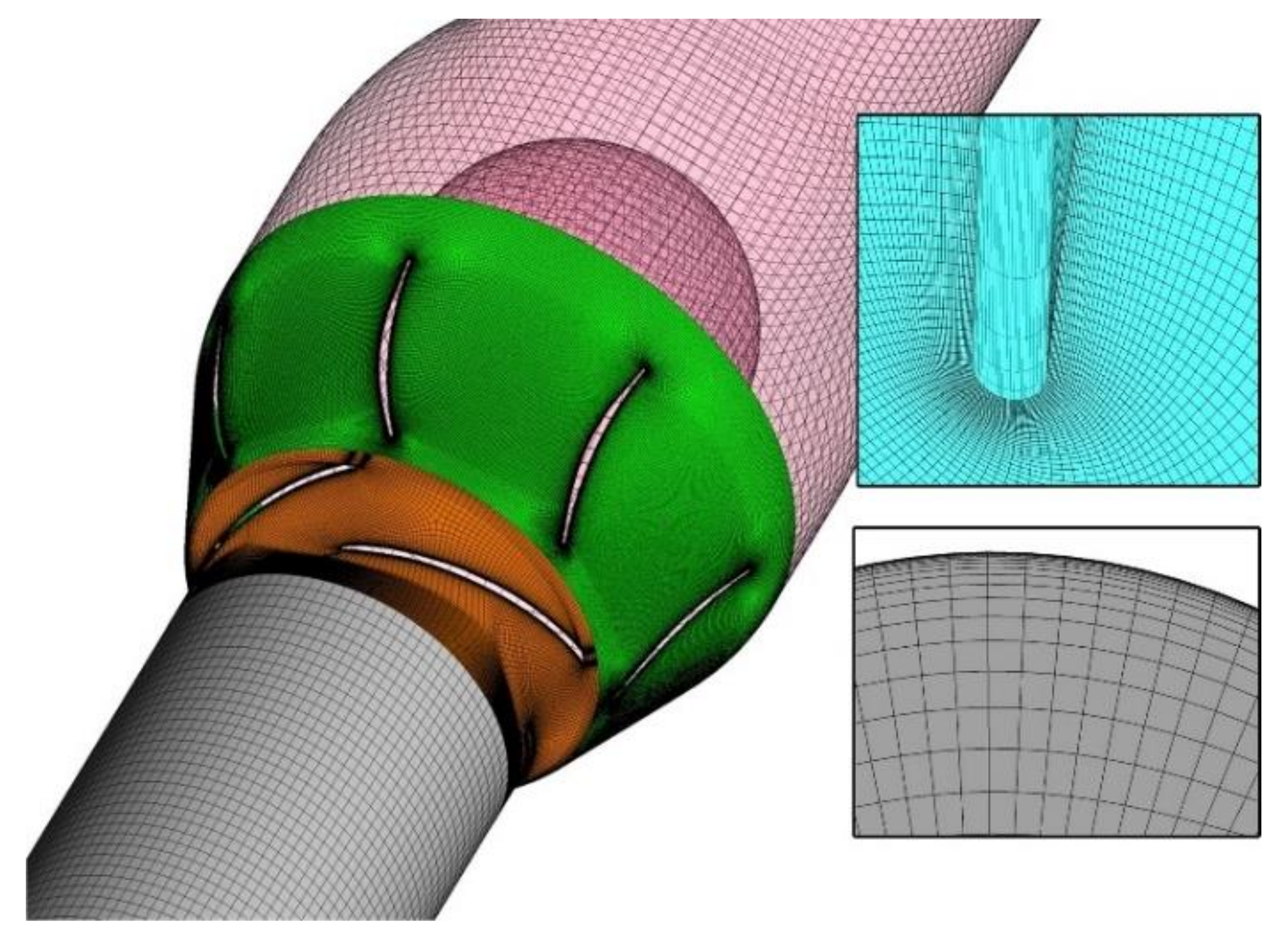
Figure 2 shows the grid system in this study. Due to the advantages in the number of grids, calculation accuracy, and convergence, hexahedral grids with high quality were used for all domains. The grids in the impeller and diffuser were generated by Turbo-Grid. For inlet and outlet pipes, ICEM with O-Block strategy was adopted to discretize the domains. To treat the high velocity gradient, all near wall surfaces were refined with prism layers. The expansion ratio of near wall grids is 1.2. The first layer nodes distance was controlled to ensure the dimensionless distance, y+ < 50 [24], which could meet the need of the grid for the SST k–ω turbulence model.
A grid independent check (GIC) was conducted to make sure that the simulations in the optimization process are free from errors caused by the grid number. The results of the GIC are shown in Table 2, and the grid refinement factor is approximately 1.3. When the grid number increases from 7.63 million to 9.92 million, the relative error of head is 0.24%. Finally, the grid number of 7.63 million was used for subsequent optimizations and simulations.
The comparison of the head and efficiency curves is shown in Figure 3. The CFD curves are obtained by steady simulations. The tested performance curves were acquired from an experimental study presented in Section 4.4. As the mechanical and volumetric efficiency were not considered in simulations, the results obtained by CFD are generally higher than the experimental values. The maximum relative errors of the head and hydraulic efficiency are lower than 5%. The absolute predicted deviations for the head and hydraulic efficiency at the design condition are 0.55 m and 3.83%, respectively. Thus, the numerical accuracy is suitable for the following optimization study.
2.3. Entropy Generation Theory
Entropy is one of the physical qualities that characterize the state of matter in thermodynamics. The nature of entropy indicates the chaos inside the system. The entropy generation theory is proposed based on the second law of thermodynamics, which effectively explains the flow direction and loss of energy. Flow losses in fluid machinery are very complex as total pressure loss cannot visualize and locate the maximum flow loss in pumps. To explain the influence of the optimization variable on hydraulic performance, the details of flow loss in the pump are revealed in depth. A visualization method of flow loss based on the entropy generation theory was proposed. The transfer equation of entropy for incompressible fluid can be described as [25]:
where s is the specific entropy, T is the thermodynamic temperature, and u, v, and w are the Cartesian velocity components, is the heat flux density vector, and represent the entropy generation rate caused by dissipation and heat transfer, respectively.
According to the Reynolds averaged Navier Stokes (RANS) approach for turbulent flows, prior to time-averaging the equation, all quantities are split into time-mean and fluctuating parts; thus, the time-averaged governing equation then reads [25]:
In this research, the heat transfer is neglected; hence, only the entropy generation by dissipation () is considered. The time average format of entropy generation can be expressed as [26]:
where , , and represent the time-averaged velocity components, and , , and are the velocity fluctuation components.
The first term, , which includes the average velocity gradient, can be interpreted as the entropy generation dissipated in the average flow field. The second term,, which contains the gradients of the fluctuating velocities, cannot be obtained directly; thus, it is often called indirect or turbulent dissipation. Herwig et al. [27] found that there is a close relationship between this term and turbulent eddy dissipation. Thus, the is defined as:
Because of the viscosity, there is a large velocity gradient near the wall. The time average variables are obviously affected by the effect of the wall surface, and it is hard to solve them accurately. Therefore, Hou et al. [28] proposed a new method to calculate the wall entropy production rate:
where represents the shear force on the wall, and V is the average velocity vector of the first layer of the grid near the wall surface.
By the volume and surface integration, the entropy generation power of each term can be calculated [29]:
The total volume entropy generation power (Pv) is defined as the sum of Equations (10) and (11) [29]:
All the statistical variables in Equations (6) and (8) were arithmetically averaged in the last revolution of the impeller.
3. Optimizing Method
To reduce the human factor and shorten the optimization time, a highly integrated optimization platform was established. Figure 4 shows the procedure of this optimization. The entire optimization process mainly consists of two stages. The main task of the first stage is to establish accurate surrogate models. In this process, the DOE method combined with the CFD method was used for sampling in m-dimensional space. Regression analysis was introduced to test the accuracy of the surrogate models. If the accuracy is lower than the threshold value, DOE will be repeatedly performed until satisfactory results are obtained. Secondly, the optimal solution was obtained by solving the surrogate models with MIGA. The optimization platform was established by the integration of CFturbo, Turbo-Grid, ICEM, and CFX. Disk Operating System (DOS) commands and script files were used to run the software in the background. The DOE program was used to drive the platform.
3.1. Mathematical Model
The main purpose of this optimization is to improve the hydraulic efficiency, which belongs to the single objective optimization. The mathematical model of this problem is as follow:
maximize
subject to
where η is the hydraulic efficiency under the design flow rate, is the vector of the m design variables. Both the meridional and blade shape of the impeller and diffuser were optimized in this study. The definition of the geometric parameters is shown in Figure 5. The meridional shape of the flow passage in optimized schemes was formed by multipoint Bezier curves, while the benchmark design adopts arcs and straight lines. To reduce the number of optimization variables appropriately, some parameters are reasonably constrained: β1, β2, φb, α3, and φd vary linearly from hub to shroud, b3 is strictly equal to b2, while α4 is consistent from hub to shroud. Finally, 14 were selected for the optimization. Table 3 shows the ranges of the optimization variables.
3.2. Design of Experiment
The Latin hypercube experimental design is an efficient experimental design method with the advantages of effective space filling and the ability to fit second-order or more nonlinear relationships. The optimal Latin hypercube (OLH) improves the uniformity of the Latin hypercube and makes all sampling points more evenly distributed in the design space [30]. To establish more accurate surrogate models, the OLH was used to perform the space sampling. The number of samples is related to the accuracy of the surrogate model. An accurate model requires enough sampling points; however, too many sampling points will consume a lot of time. For tradeoffs between model accuracy and sampling time, the regression analysis was performed using the coefficient of determination R2 after DOE. The closer R2 is to 1, the more accurate the model will be. Usually R2 is greater than 0.9 [31]. To ensure the accuracy of the surrogate model, if the value of R2 is below the threshold value (0.96), additional sampling points will be added. Within each modeling process, 50 sampling points were added. R2 is defined as follows [31]:
where n is the number of samples, represents the average response, is the predicted value, and is the actual value.
3.3. RBF Neural Network
The artificial neural network (ANN) is a kind of bionic computing system, which has good, nonlinear fitting, learning and updating abilities; hence, it is widely used in machine learning, optimization design, and other fields. The radial basis function (RBF) is one kind of a three layer forward neural network. Figure 6 shows the structure of the RBF [32]. It consists of three layers: input layer, hidden layer, and output layer. In the RBF neural network, the input vector is directly mapped to the hidden layer through the function, and there is no need to adjust the connection weights.
The independent variable of the RBF is the Euclidean distance between the test point and the sample point. The output of hidden layer is [32]:
where ci is the center vector of the Gaussian function, and σi represents the width of the ith Gaussian function.
The output layer responds to the action of the input mode, and there is a linear mapping from the output R(xm) of the hidden layer to the output layer y [32]:
where ωi is the weight between the hidden layer and the output layer.
3.4. MIGA Algorithm
The genetic algorithm (GA) is a very classical algorithm widely used in multidisciplinary optimization. It was first proposed in 1971 based on the rule of „survival of the fittest” in Darwin’s evolution theory [33]. The algorithm imitates the genetic reproduction mechanism of organisms; regards the solution space as a population with a certain principle used to encode individuals in the population; and then genetic operations on the encoded individuals was performed. The main search steps of GA include: selection, crossover, mutation, and so on. The offspring or mutated individuals replace the old population using the elitism or diversity replacement strategy and form as the new population in the next generation. The optimal solution will be obtained from the new population through iteration, which can effectively solve the problems of large-scale combination optimization or discontinuous search space. GA is one of the most prominent stochastic optimization algorithms.
After years of development, there are many types of genetic algorithms. Among them, parallel distributed genetic algorithms (PDGAs) are the most popular ones. Further, Miki et al. [34] made improvements on the PDGAs, and they divided the solution space into many parts called “islands”. When performing the optimization, some individuals are selected on each “island” to conduct optimization according to the principle of the GA, and then migrate to other “islands” for the same operation at certain intervals. This is the so called MIGA. Compared with the traditional GA, the migration operation was added in MIGA. The biggest advantage of MIGA is that it is good at global search and can avoid falling into the local optimal solution. Figure 7 shows the structure of MIGA. The algorithm settings are shown in Table 4. A total of 4000 iterations were executed.
4. Results and Discussions
4.1. Regression Analysis
After repeating the experimental design five times, the accuracy of the model reached the requirements. Therefore, 250 sampling points were used to establish the RBF model. Figure 8 shows the results of the DOE. The objective variables show great fluctuations in the solution space. The maximum difference in head exceeds 3.5 m, the fluctuation amplitude of efficiency is larger than 3.5%. Therefore, the value ranges of variables are suitable for optimization.
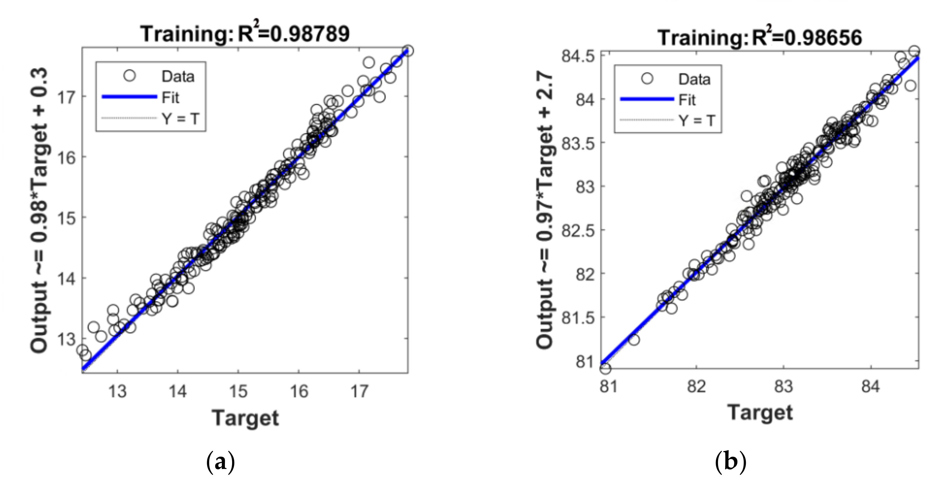
The accuracy of the surrogate model was evaluated by regression analysis. Figure 9 shows the R2 of both the head and efficiency, and they are all larger than 0.98. Therefore, the accuracy of these two models is sufficient for further optimization.
4.2. Sensitivity Analysis
Sensitivity analysis is a method to study the influence of input parameters on output in a system. The sensitivity coefficients help the designer decide which parameters can be ignored in the product optimization. Correlation analysis is a linear analysis method based on the Pearson and Spearman correlation. The correlation coefficient, r, between two variables can be calculated as follows [35]:
It can be seen that r ranges from −1 to 1, and when r > 0, the two variables are positively correlated; otherwise, they are negatively correlated. It is generally believed that when the absolute value of the correlation coefficient is greater than 0.4, there is a significant correlation between the two variables. Correlation analysis is an effective tool to evaluate the influence of variables on the target and helps designers reduce the number of optimization variables.
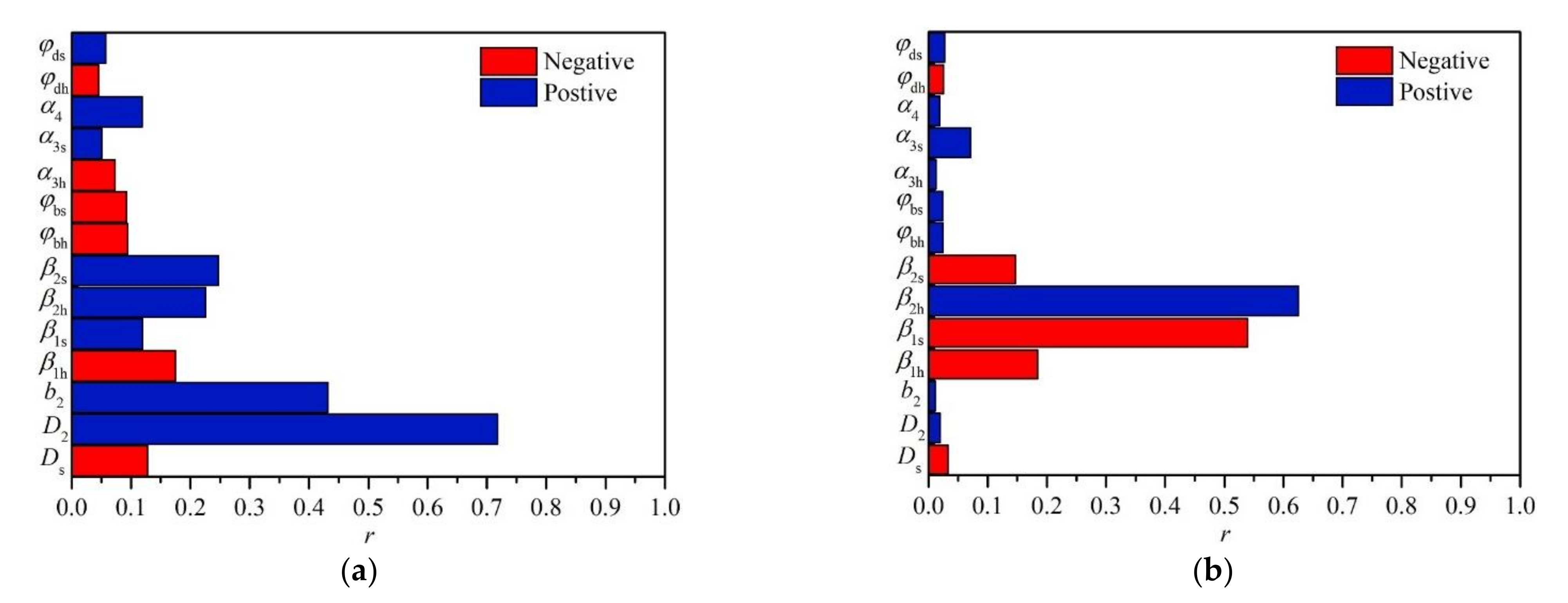
Figure 10 shows the effects of the optimization variables on the pump head and efficiency. The blue bars indicate the positive effects and the red bars present the negative effects. The results show that b2 and D2 have a significant positive effect on the design head. This means that increasing the impeller outlet width and outlet diameter can significantly increase the design head of the mixed flow pump. In addition, the blade outlet angles also have an obvious positive effect on the design head, while φdh, φds, and α3s can be ignored with very small correlation coefficients. For the pump efficiency, the impeller blade shape plays an important role, especially the inlet and outlet angles. The blade outlet hub angle, β2h, has the greatest positive effect on the pump efficiency. Reducing the blade inlet angle within this constraint is beneficial to improve the pump efficiency. However, efficiency is less sensitive to other parameters.
4.3. Optimization Results
By solving the RBF surrogate models, the best solution was obtained. Table 5 shows the comparison of geometric parameters between the initial and optimized schemes. The 3D geometry comparison of the mixed impeller and vaned diffuser between the initial design and the optimal scheme is shown in Figure 11. The results predicted by the surrogate models are compared with CFD in Table 6. The relative errors of the head and efficiency between the predicted values and the CFD results are 0.82% and 0.33%, respectively. Compared with the initial scheme, the efficiency under the design condition increased by 5.1%, while the deviation of head is within 0.5 m.
Figure 12 shows the comparison of the velocity streamline in the impeller and guide blade runner in different spanwise. The incident angle of the blade inlet shows that there is a large inflow impact near the blade leading edge (LE) of the initial scheme, especially at span = 20%. When the flow angle is less than the blade inlet angle, flow separation occurs on the suction side (SS), increasing the velocity and flow loss near the LE. With the decrease of the blade inlet angle in the optimized scheme, the inflow direction almost fits the blade profile, the flow separation on the SS was effectively suppressed, and the velocity distribution is more uniform. In addition, the flow regime in the diffuser has also been improved. For the initial scheme, there are large-scale, low-speed regions and separation vortexes near the hub, causing serious blockage near the diffuser outlet. With the increase of spanwise, the separation vortexes move towards the diffuser outlet, and their scale decreases gradually. With the increase of the vane wrap angle, the separation phenomenon in the optimized scheme is greatly improved. Although some separation vortexes still remain at 20% spanwise, their numbers and sizes are significantly reduced. The streamlines at 80% spanwise completely align with the blade profile, and the flow separation phenomenon disappears.
According to the entropy generation theory, turbulent eddy dissipation (TED) is one of the important factors causing flow loss in the pump. Figure 13 shows the distribution of average TED at different spanwise. The TED at span = 20% and span = 50% in Figure 13a,b indicate that the flow separation on the blade SS is prone to cause dissipation loss. With the increase of spanwise, the effect of the rotor–stator interaction increased, the TED peak on the blade SS moves towards the blade TE, and the TED in the diffuser increased. Figure 13d–f illustrate that the TED on the blade surface is significantly reduced in the optimized scheme. In addition, the TED in the diffuser at span = 50% and span = 80% also decreased to a certain extent.
Figure 14 shows the comparison of volume entropy generation. The value of entropy generation reflects the magnitude of flow loss. Consistent with the results reflected in Figure 12 and Figure 13, the peak value of entropy generation in the impeller was observed near the LE on the SS in the initial scheme, and the entropy generation fades away along the streamwise. Entropy generation in the diffuser is mainly distributed in the low-speed regions; thus the flow separation diffuser is the main cause of the diffusion loss. After optimization, entropy generation on the blade surfaces is almost eliminated, and the impeller efficiency is improved. In the diffuser, the entropy generation near the hub was still obvious in the optimized scheme, while the flow loss near the shroud is reduced, which contributes to the improvement of the energy recovery rate of the diffuser.
By volume integral of entropy generation S, the total volume entropy generation power Pv of impeller and diffuser were obtained. Similar to total pressure drop, Pv represents the magnitude of flow loss in a domain. Figure 15 compares Pv in the impeller and diffuser, the flow loss in the impeller is greater than that in the diffuser. The optimization results show that Pv in the impeller and diffuser decreased by 33.3% and 19.0%, respectively. The decrease of entropy generation in the impeller is the main reason for the efficiency improvement.
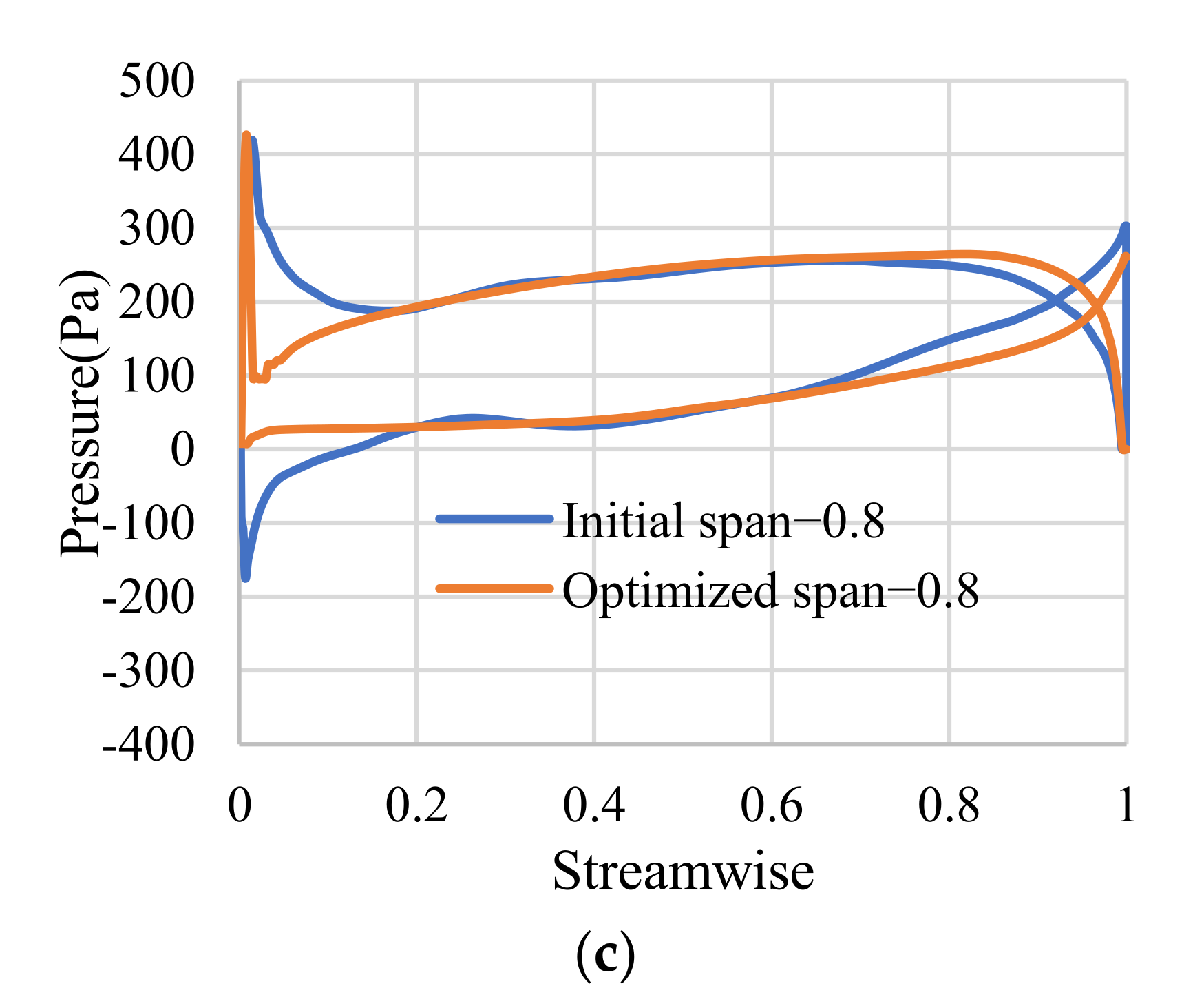
Figure 16 shows the blade loading on different spanwise along the streamwise. The blade loading increases along the spanwise. The blade shape near the shroud has the greatest influence on the impeller performance. The difference is mainly found near the LE and TE. A pressure jump is observed near the TE because of the cut off. Owing to the serious flow separation near the LE of the initial scheme, the relative larger pressure difference appears in front of the blade (streamwise: 0~0.2). Additionally, the decrease of blade loading initiated before 80% streamwise. For the optimized scheme, the blade loading before 20% streamwise is greatly improved. In addition, the minimum differential pressure is closer to the TE, and the blade loading is more uniformly distributed along the streamwise.
4.4. Experimental Verification
To verify the optimization results, the hydraulic components were manufactured, and performance tests were carried out on the opening test rig. Figure 17a presents the test site of the mixed pump, and it mainly includes the tested pump, motor, pipes and so on. The pump was installed horizontally, and an elbow pipe was used to connect the pump and outlet pipe. The pump head was measured by a differential pressure transducer whose accuracy is better than 0.1%. The volume flow was measured by the electromagnetic flowmeter with an uncertainty of 0.2%. The input power of the pump was calculated according to the motor efficiency curve. The error of shaft power is less than 0.14%. The systematic uncertainty of the test rig is 0.26%, which meets the level 1 accuracy requirements specified in ISO9906-2012.
The performance curves of the initial and optimized schemes are compared in Figure 18. After optimization, the head and pump efficiency increased under the full flow condition. The maximum pump efficiency increased by 4.7%, and the best efficiency point shifts to large flow. At the same time, the optimization scheme alleviates the problem of the rapid drop of the head and efficiency curves under large flow conditions and broadens the high efficient operation range.
5. Conclusions
A vaned mixed flow pump was optimized by MIGA. An intelligent optimization platform integrating DOE, mesh generation, numerical simulation, and RBF neural network were established to shorten the optimization time. The best solution was obtained by solving the RBF model. This research has reached the following conclusions:
- The RBF neural network has good accuracy in terms of the complex nonlinear relationships. The R2 value of both the head and efficiency under the design condition is better than 0.98. The relative error between the predicted values and the CFD results is less than 1%.
- The impeller outlet width, b2, and its outlet diameter, D2, have a significant positive effect on the design head, while the efficiency is more sensitive to the blade angles.
- The efficiency of the optimized scheme predicted by CFD increased by 5.1%. Experimental results show that the maximum pump efficiency increased by 4.7%, and the high efficient operation range is significantly broadened.
- The entropy generation can effectively visualize the flow loss distribution caused by turbulent dissipation and flow separation. Compared with the initial scheme, the volume entropy generation powers in the impeller and diffuser are effectively reduced, and the blade loading is more uniformly distributed along the streamwise.
- The optimization platform proposed in this study is universal and can be applied to conduct optimization of other fluid machinery.
Author Contributions
Data curation, R.L.; validation, J.Y. and Q.S.; formal analysis, Q.S.; funding acquisition, G.W. and Y.Z.; investigation, J.Y.; resources, X.L.; supervision, J.Y.; writing—original draft preparation, R.L.; writing—review and editing, Q.S. All authors have read and agreed to the published version of the manuscript.
Funding
This research was funded by the National Key Research and Development Program of China (2020YFC1512403) and the National Natural Science Foundation of China (51976079).
Institutional Review Board Statement
Not applicable.
Informed Consent Statement
Not applicable.
Data Availability Statement
Not applicable.
Conflicts of Interest
The authors declare no conflict of interest.
Nomenclature
| uvw | Cartesian velocity components |
| xyz | Coordinate components |
| t | Time |
| f | Body force |
| p | Pressure |
| μ | Dynamic viscosity |
| P | Entropy generation power |
| T | Temperature |
| D2 | Impeller outlet diameter |
| Ds | Impeller suction diameter |
| b | Width |
| α | Diffuser van angle |
| β | Impeller blade angle |
| φ | Wrap angle |
| Q | Flow rate |
| n | Rotational speed |
| m | Sample number |
| V | Volume |
| Ω | Area |
| H | Head |
| s | Entropy |
| Viscous dissipation | |
| Turbulent dissipation | |
| Heat flux density vector | |
| θ | Volute tongue angle |
| α | Circumferential angle |
| ρ | Density |
| ν | Kinematic viscosity |
| ε | Turbulent Eddy Dissipation |
| Subscripts | |
| 1 | Impeller inlet |
| 2 | Impeller outlet |
| 3 | Diffuser inlet |
| 4 | Diffuser outlet |
| i | Free index |
| j | Dummy index |
| h | Hub |
| s | Shroud |
| b | Blade |
| d | Diffuser |
| Superscripts | |
| ¯ | Time-averaged value |
| ′ | Fluctuating component |
References
- Bozorgasareh, H.; Kh Alesi, J.; Jafari, M.; Gazori, H.A. Performance improvement of mixed-flow centrifugal pumps with new impeller shrouds: Numerical and experimental investigations. Renew. Energ. 2021, 163, 635–648. [Google Scholar] [CrossRef]
- Kim, S.; Kim, Y.I.; Kim, J.H.; Choi, Y.S. Design optimization for mixed-flow pump impeller by improved suction performance and efficiency with variables of specific speeds. J. Mech. Sci. Technol. 2020, 34, 2377–2389. [Google Scholar] [CrossRef]
- Hao, B.; Cao, S.L.; Tan, L.; Zhu, B.S. Effects of meridional flow passage shape on hydraulic performance of mixed-flow pump impellers. Chin. J. Mech. Eng. 2013, 7, 469–475. [Google Scholar]
- Ji, L.L.; Li, W.; Shi, W.D.; Tian, F.; Agarwal, R. Effect of blade thickness on rotating stall of mixed-flow pump using entropy generation analysis. Energy 2021, 236, 121381. [Google Scholar] [CrossRef]
- Ikuta, A.; Nitta, N.; Miyagawa, K.; Shinozuka, Y.; Tomimatsu, S. Influence of forward skew blade angle on positive slope characteristics of mixed flow pumps. J. Phys. Conf. Ser. 2021, 1909, 012076. [Google Scholar] [CrossRef]
- Li, W.; Ji, L.L.; Li, E.D.; Zhou, L.; Agarwal, R.K. Effect of tip clearance on rotating stall in a mixed-flow pump. J. Turbomach. 2021, 143, 091013. [Google Scholar] [CrossRef]
- Han, Y.D.; Tan, L. Influence of rotating speed on tip leakage vortex in a mixed flow pump as turbine at pump mode. Renew. Energ. 2021, 162, 144–150. [Google Scholar] [CrossRef]
- Wang, L.K.; Lu, J.L.; Liao, W.L.; Guo, P.C.; Feng, J.J.; Luo, X.Q.; Wang, W. Numerical investigation of the effect of t-shaped blade on the energy performance improvement of a semi-open centrifugal pump. J. Hydrodyn. 2021, 33, 736–746. [Google Scholar] [CrossRef]
- Zhu, X.Y.; Li, G.J.; Jiang, W.; Fu, L. Experimental and numerical investigation on application of half vane diffusers for centrifugal pump. Int. Commun. Heat Mass Transf. 2016, 79, 114–127. [Google Scholar] [CrossRef]
- Khoeini, D.; Shirani, E.; Joghataei, M. Improvement of centrifugal pump performance by using different impeller diffuser angles with and without vanes. J. Mech. 2019, 35, 577–589. [Google Scholar] [CrossRef]
- Wang, W.J.; Yuan, S.Q.; Pei, J.; Zhang, J.F. Optimization of the diffuser in a centrifugal pump by combining response surface method with multi-island genetic algorithm. Proc. Inst. Mech. Eng. Part E J. Process Mech. Eng. 2017, 231, 191–201. [Google Scholar] [CrossRef]
- Kim, J.H.; Kim, K.Y. Analysis and optimization of a vaned diffuser in a mixed flow pump to improve hydrodynamic performance. J. Fluids Eng. 2012, 134, 071104. [Google Scholar] [CrossRef]
- Wang, M.C.; Li, Y.J.; Yuan, J.P.; Osman, F.K. Influence of Spanwise Distribution of Impeller Exit Circulation on Optimization Results of Mixed Flow Pump. Appl. Sci 2021, 11, 507. [Google Scholar] [CrossRef]
- Wang, M.C.; Li, Y.J.; Yuan, J.P.; Osman, F.K. Matching optimization of a mixed flow pump impeller and diffuser based on the inverse design method. Processes 2021, 9, 260. [Google Scholar] [CrossRef]
- Lu, Y.M.; Wang, X.F.; Wang, W.; Zhou, F.M. Application of the modified inverse design method in the optimization of the runner blade of a mixed-flow pump. Chin. J. Mech. Eng. 2018, 31, 127–143. [Google Scholar] [CrossRef] [Green Version]
- Bonaiuti, D.; Zangeneh, M.; Aartojarvi, R.; Eriksson, J. Parametrical Design of a Waterjet Pump by Means of Inverse Design, CFD Calculations and Experimental Analyses. J. Fluids Eng. 2010, 132, 201–215. [Google Scholar] [CrossRef]
- Ye, W.X.; Geng, C.; Ikuta, A.; Hachinota, S.; Miyagawa, K.; Luo, X.W. Investigation on the impeller-diffuser interaction on the unstable flow in a mixed-flow pump using a modified partially averaged Navier-Stokes model. Ocean Eng. 2021, 238, 109756. [Google Scholar] [CrossRef]
- Wang, W.J.; Pei, J.; Yuan, S.Q.; Zhang, J.F.; Yuan, J.P.; Xu, C.Z. Application of different surrogate models on the optimization of centrifugal pump. J. Mech. Sci. Technol. 2016, 30, 567–574. [Google Scholar] [CrossRef]
- Si, Q.R.; Lu, R.; Shen, C.H.; Xia, S.J.; Yuan, J.P. An intelligent CFD-based optimization system for fluid machinery: Automotive electronic pump case application. Appl. Sci. 2020, 10, 366. [Google Scholar] [CrossRef] [Green Version]
- Wu, X.F.; Tian, X.; Tan, M.G.; Liu, H.L. Multi-parameter optimization and analysis on performance of a mixed flow pump. J. Appl. Fluid Mech. 2020, 13, 199–209. [Google Scholar] [CrossRef]
- Pei, J.; Wang, W.J.; Osman, M.K.; Gan, X.C. Multiparameter optimization for the nonlinear performance improvement of centrifugal pumps using a multilayer neural network. J. Mech. Sci. Technol. 2019, 33, 2681–2691. [Google Scholar] [CrossRef]
- Zhu, D.; Tao, R.; Xiao, R.F.; Yang, W.; Liu, W.C.; Wang, D.J. Optimization design of hydraulic performance in vaned mixed-flow pump. Proc. Inst. Mech. Eng. Part A J. Pow. Energ. 2019, 234, 934–946. [Google Scholar] [CrossRef]
- Huang, R.F.; Luo, X.W.; Ji, B.; Wang, P.; Yu, A.; Zhai, Z.H.; Zhou, J.J. Multi-objective optimization of a mixed-flow pump impeller using modified NSGA-II algorithm. Sci. China Technol. Sci. 2015, 58, 2122–2130. [Google Scholar] [CrossRef]
- Zhang, F.; Appiah, D.; Hong, F.; Zhang, J.F.; Yuan, S.Q.; Adu-Poku, K.A.; Wei, X.Y. Energy loss evaluation in a side channel pump under different wrapping angles using entropy production method. Int. Commun. Heat Mass Transf. 2020, 113, 104526. [Google Scholar] [CrossRef]
- Lu, R.; Yuan, J.P.; Wang, L.Y.; Fu, Y.X.; Hong, F.; Wang, W.J. Effect of volute tongue angle on the performance and flow unsteadiness of an automotive electronic cooling pump. Proc. Inst. Mech. Eng. Part A J. Pow. Energ 2020, 235, 227–241. [Google Scholar] [CrossRef]
- Gu, Y.D.; Pei, J.; Yuan, S.Q.; Wang, W.J.; Zhang, F.; Wang, P.; Appiah, D.; Liu, Y. Clocking effect of vaned diffuser on hydraulic performance of high-power pump by using the numerical flow loss visualization method. Energy 2019, 170, 986–997. [Google Scholar] [CrossRef]
- Herwig, H.; Schmandt, B. How to determine losses in a flow field: A paradigm shift towards the second law analysis. Entropy 2014, 16, 2959–2989. [Google Scholar] [CrossRef] [Green Version]
- Hou, H.C.; Zhang, Y.X.; Li, Z.L.; Jiang, T.; Zhang, J.Y.; Xu, C. Numerical analysis of entropy production on a LNG cryogenic submerged pump. J. Nat. Gas Sci. Eng. 2016, 36, 87–96. [Google Scholar] [CrossRef]
- Lin, T.; Li, X.J.; Zhu, Z.C.; Xie, J.; Li, Y.; Yang, H. Application of enstrophy dissipation to analyze energy loss in a centrifugal pump as turbine. Renew. Energy 2021, 163, 41–55. [Google Scholar] [CrossRef]
- Lu, R.; Yuan, J.P.; Li, Y.J.; Jiang, H.Y. Automatic optimization of axial flow pump based on radial basis functions neural network and CFD. JDIME 2017, 35, 481–487. [Google Scholar]
- Moriasi, D.N.; Arnold, J.G.; Van Liew, M.W.; Bingner, R.L.; Harmel, R.D.; Veith, T.L. Model evaluation guidelines for systematic quantification of accuracy in watershed simulations. ASABE 2007, 50, 885–900. [Google Scholar] [CrossRef]
- Li, T.S.; Duan, S.K.; Liu, J.; Wang, L.D. An improved design of RBF neural network control algorithm based on spintronic memristor crossbar array. Neural Comput. Appl. 2018, 30, 1939–1946. [Google Scholar] [CrossRef]
- Sinha, A.; Malo, P.; Deb, K. Evolutionary algorithm for bilevel optimization using approximations of the lower level optimal solution mapping. Eur. J. Oper. Res. 2017, 257, 395–411. [Google Scholar] [CrossRef]
- Miki, M. A parallel genetic algorithm with distributed environment scheme. In Proceedings of the IEEE International Conference on Systems, Man and Cybernetics, Tokyo, Japan, 12–15 October 1999; IEEE: Piscataway, NJ, USA, 1999; pp. 695–700. [Google Scholar]
- Li, Z.P.; Gao, X.J.; Lu, D.G. Correlation analysis and statistical assessment of early hydration characteristics and compressive strength for multi-composite cement paste. Constr. Build. Mater. 2021, 310, 125260. [Google Scholar] [CrossRef]
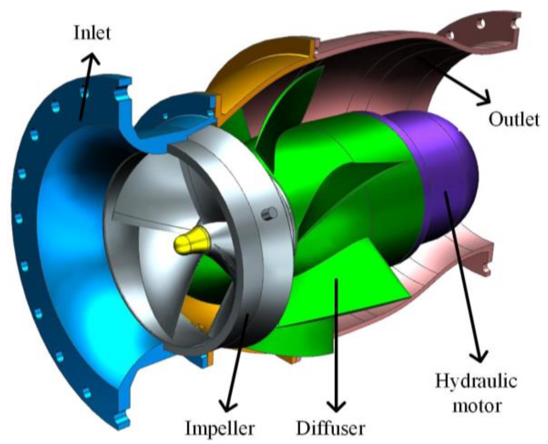
Figure 1.
Structure of Mixed Flow Pump.

Figure 2.
Hexahedral mesh of computational domains.

Figure 3.
Comparison of performance curves.

Figure 4.
Procedure of the optimization design.

Figure 5.
Schematic diagram of geometric parameters. (a) Definition of meridional parameters. (b) Definition of impeller blade angles. (c) Definition of diffuser vane angles.
Figure 5.
Schematic diagram of geometric parameters. (a) Definition of meridional parameters. (b) Definition of impeller blade angles. (c) Definition of diffuser vane angles.

Figure 6.
Principle of RBF neural network.

Figure 7.
Structure of MIGA.

Figure 8.
Results of DOE. (a) Head. (b) Efficiency.

Figure 9.
Regression analysis of surrogate models. (a) R2 of head. (b) R2 of efficiency.

Figure 10.
Correlation analysis for objectives. (a) Effect on head. (b) Effect on efficiency.

Figure 11.
Geometric comparison of impeller and diffuser. (a) Initial scheme. (b) Optimized scheme.

Figure 12.
Velocity and streamline distribution in different spanwise. (a) Initial scheme at span = 20%. (b) Initial scheme at span = 50%. (c) Initial scheme at span = 80%. (d) Optimized scheme at span = 20%. (e) Optimized scheme at span = 50%. (f) Optimized scheme at span = 80%.
Figure 12.
Velocity and streamline distribution in different spanwise. (a) Initial scheme at span = 20%. (b) Initial scheme at span = 50%. (c) Initial scheme at span = 80%. (d) Optimized scheme at span = 20%. (e) Optimized scheme at span = 50%. (f) Optimized scheme at span = 80%.

Figure 13.
Turbulence eddy dissipation in different spanwise. (a) Initial scheme at span = 20%. (b) Initial scheme at span = 50%. (c) Initial scheme at span = 80%. (d) Optimized scheme at span = 20%. (e) Optimized scheme at span = 50%. (f) Optimized scheme at span = 80%.
Figure 13.
Turbulence eddy dissipation in different spanwise. (a) Initial scheme at span = 20%. (b) Initial scheme at span = 50%. (c) Initial scheme at span = 80%. (d) Optimized scheme at span = 20%. (e) Optimized scheme at span = 50%. (f) Optimized scheme at span = 80%.


Figure 14.
Comparison of volume entropy production power in different spanwise. (a) Initial scheme at span = 20%. (b) Initial scheme at span = 50%. (c) Initial scheme at span = 80%. (d) Optimized scheme at span = 20%. (e) Optimized scheme at span = 50%. (f) Optimized scheme at span = 80%.
Figure 14.
Comparison of volume entropy production power in different spanwise. (a) Initial scheme at span = 20%. (b) Initial scheme at span = 50%. (c) Initial scheme at span = 80%. (d) Optimized scheme at span = 20%. (e) Optimized scheme at span = 50%. (f) Optimized scheme at span = 80%.

Figure 15.
Comparison of the total volume entropy generation power. (a) Pv of impeller. (b) Pv of diffuser.
Figure 15.
Comparison of the total volume entropy generation power. (a) Pv of impeller. (b) Pv of diffuser.

Figure 16.
Distribution of blade loading. (a) Span = 20%. (b) Span = 50%. (c) Span = 80%.


Figure 17.
Experimental measurement. (a) Test rig. (b) Impeller. (c) Diffuser.

Figure 18.
Comparison of experimental performance curves between initial and optimized schemes.


Table 1.
Design specifications of the mixed flow pump.
| Parameters | Symbols | Values |
|---|---|---|
| Rate flow | Q | 3500 m3/h |
| Rotational speed | n | 1500 r/min |
| Head | H | 16 m |
| Impeller suction diameter | Ds | 380 mm |
| Impeller outlet diameter | D2 | 340 mm |
| Impeller outlet width | b2 | 125 mm |
| Diffuser inlet width | b3 | 125 mm |
| Diffuser outlet angle | α4 | 90° |
Table 2.
Grid independence check.
| Grid Number (Million) | H (m) | Relative Error (%) |
|---|---|---|
| 3.47 | 14.87 | - |
| 4.52 | 15.75 | 5.91% |
| 5.87 | 16.15 | 2.54% |
| 7.63 | 16.39 | 1.49% |
| 9.92 | 16.43 | 0.24% |
Table 3.
Ranges of optimization parameters.
| Optimization Parameters | Lower Bound | Baseline | Upper Bound |
|---|---|---|---|
| Impeller suction diameter Ds (mm) | 360 | 380 | 390 |
| Impeller outlet diameter D2 (mm) | 330 | 340 | 350 |
| Impeller outlet width b2 (mm) | 120 | 125 | 130 |
| Inlet angle of blade hub β1h (deg) | 35 | 37 | 50 |
| Inlet angle of blade shroud β1s (deg) | 10 | 15 | 25 |
| Outlet angle of blade hub β2h (deg) | 20 | 23 | 35 |
| Outlet angle of blade shroud β2s (deg) | 30 | 35 | 45 |
| Wrap angle of blade hub φbh (deg) | 90 | 102 | 110 |
| Wrap angle of blade shroud φbs (deg) | 85 | 91 | 95 |
| Inlet angle of vane hub α3h (deg) | 35 | 41 | 50 |
| Inlet angle of vane shroud α3s (deg) | 45 | 52 | 60 |
| Vane outlet angle α4 (deg) | 85 | 90 | 92 |
| Wrap angle of vane hub φdh (deg) | 30 | 34 | 40 |
| Wrap angle of vane shroud φds (deg) | 15 | 19 | 25 |
Table 4.
Parameters adopted in MIGA.
| Parameters | Value |
|---|---|
| Number of generations | 10 |
| Sub-population size | 20 |
| Number of islands | 20 |
| Rate of crossover | 0.9 |
| Rate of migration | 0.01 |
| Interval of migration | 5 |
| Rate of mutation | 0.01 |
Table 5.
Comparison of geometric parameters.
| Parameters | Initial | Optimized |
|---|---|---|
| Ds (mm) | 380 | 385.7 |
| D2 (mm) | 340 | 341.1 |
| b2 (mm) | 125 | 129.4 |
| β1h (°) | 37 | 35.7 |
| β1s (°) | 15 | 10.1 |
| β2h (°) | 23 | 34.8 |
| β2s (°) | 35 | 30.4 |
| φbh (°) | 102 | 109.5 |
| φbs (°) | 91 | 94.8 |
| α3h (°) | 41 | 42.9 |
| α3s (°) | 52 | 58.1 |
| α4 (°) | 90 | 90.2 |
| φdh (°) | 34 | 30.7 |
| φds (°) | 19 | 24.7 |
Table 6.
Comparison of performance under design condition.
| Case | Method | Head (m) | Efficiency (%) |
|---|---|---|---|
| Initial | CFD | 16.39 | 80.26 |
| Optimized | RBF | 17.02 | 85.63 |
| CFD | 16.88 | 85.36 |
Publisher’s Note: MDPI stays neutral with regard to jurisdictional claims in published maps and institutional affiliations. |
© 2021 by the authors. Licensee MDPI, Basel, Switzerland. This article is an open access article distributed under the terms and conditions of the Creative Commons Attribution (CC BY) license (https://creativecommons.org/licenses/by/4.0/).
Share and Cite
MDPI and ACS Style
Lu, R.; Yuan, J.; Wei, G.; Zhang, Y.; Lei, X.; Si, Q. Optimization Design of Energy-Saving Mixed Flow Pump Based on MIGA-RBF Algorithm. Machines 2021, 9, 365. https://doi.org/10.3390/machines9120365
AMA Style
Lu R, Yuan J, Wei G, Zhang Y, Lei X, Si Q. Optimization Design of Energy-Saving Mixed Flow Pump Based on MIGA-RBF Algorithm. Machines. 2021; 9(12):365. https://doi.org/10.3390/machines9120365
Chicago/Turabian StyleLu, Rong, Jianping Yuan, Guangjuan Wei, Yong Zhang, Xiaohui Lei, and Qiaorui Si. 2021. "Optimization Design of Energy-Saving Mixed Flow Pump Based on MIGA-RBF Algorithm" Machines 9, no. 12: 365. https://doi.org/10.3390/machines9120365
Note that from the first issue of 2016, this journal uses article numbers instead of page numbers. See further details here.