Numerical and Experimental Investigation of the Temperature Rise of Cutting Tools Caused by the Tool Deflection Energy


1
College of Mechanical and Electrical Engineering, Nanjing University of Aeronautics and Astronautics (NUAA), Nanjing 210016, China
2
Department of Mechanical Engineering, Henan Institute Technology (HIT), Xinxiang 453003, China
*
Author to whom correspondence should be addressed.
Machines 2021, 9(6), 122; https://doi.org/10.3390/machines9060122
Submission received: 2 May 2021
/
Revised: 12 June 2021
/
Accepted: 15 June 2021
/
Published: 18 June 2021
Abstract
:Tool temperature variation in flank milling usually causes excessive tool wear, shortens tool life, and reduces machining accuracy. The heat source is the primary factor of the machine thermal error in the process of cutting components. Moreover, the accuracy of the thermal error modeling is greatly influenced by the formation mechanism of the heat source. However, the tool heat caused by the potential energy of the tool bending and twisting has essentially not been taken into consideration in previous research. In this paper, a new heat source that causes the thermal error of the cutting tools is proposed. The potential energy of the tools’ bending and twisting is calculated using experimental data, and how tool potential energy is transformed into heat via friction is explored based on the energy conservation. The temperature rise of the cutting tool is simulated by a lattice-centered finite volume method. To verify the model, the temperature separation of a tool edge is measured experimentally under the given cutting load. The results of the numerical analysis show that the rise in tool temperature caused by the tool’s potential energy is related to the time and position of the cutting edge involved in milling. For the same conditions, the predicted results are consistent with the experimental results. The proportion of temperature rise due to tool potential energy is up to 6.57% of the total tool temperature rise. The results obtained lay the foundation for accurate thermal error modeling, and also provide a theoretical basis for the force–thermal coupling process.
1. Introduction
The cutting tool is the terminal executive part of the machine tool. In metal cutting, the tool would cause the elastic–plastic deflection of the workpiece material. The energy consumed by friction between the tool, the workpiece, and the chips is converted into cutting heat [1]. Some of the heat gets transferred to the cutter. Compared with the use of coolant, the temperature rise of the local cutting area is more significant without the coolant. This increases tool wear and shortens its service life, and is an important source of errors. Therefore, the tool deflection and temperature rise problems have received focus in recent years.
Tool deflection in the cutting process is unavoidable, and the deflection energy can be transformed into heat energy. In general, the cutting tool is usually simplified as a mechanical cantilever [2]. Budak et al. [3] studied the end milling of a thin-walled part. They employed a segmented cantilever model to predict the tool deflection, and verified it with a finite element analysis. Dotcheva et al. [4] also analyzed tool deflection with a segmented cantilever beam model. The results revealed that for precision machining or micro milling of thick-walled parts, tool deflection with a small diameter and large overhang is very obvious [5]. The cutting tool has the lowest rigidity in the whole cutting system. However, the deflection energy (the potential energy of the tool) and the thermal error caused by tool deflection are rarely studied.
The heat source is another important factor affecting the tool deflection. From the perspective of the energy, there are two factors that affect the cutting temperature, i.e., the heat generation, and the heat conduction. There are three heat sources responsible for the temperature rise due to energy consumption in the cutting process [6]: (1) the heat source of the shear surface; (2) the friction heat source of the front cutting surface and chips; and (3) the friction heat source of the back cutting surface and machining surface. Research has shown that the heat source shape and the heat flow density significantly influence the precision of heat calculations [7,8]. Wang [9] established a mathematical model based on the heat source, and elaborated the generation of the cutting heat and the resulting tool temperature rise in the working. Based on a finite element cutting simulation, Putza et al. [10] were able to determine the heat energy and heat flux density. They indicated how heat flows into the workpiece, cutting tool, and chips. Wu et al. [11] put forward a method for predicting the temperature in the end mill based on an analysis model. Through the finite element simulation, the heat flux and the contact length between the cutter and the swarf were obtained. Wu et al. [12] established an analytical temperature model of cutting tools and chips in slicing, and then calculated and verified the temperature of the chips and the front cutting surface. Based on a finite difference, Islam et al. [13] devised a model of the temperature profiles in turn, and researched the instantaneous temperature distribution between the cutting tools, the workpiece surface, and the chips. In view of the Komanduri–Hou model and the Huang–Liang model, Shan et al. [14] proposed a revised cutting temperature model. Most of these cutting models are analytical or based on finite element or finite difference analysis. In fact, a finite volume model is ideal for simulating solid heat conduction in a cutting system. The form of heat source caused by tool deflection has never been mentioned.
In studies of cutting heat distribution, Reznikov and Kato [15,16] researched the effect of cutting speed on the cutting heat distribution. The highest cutting speeds had the highest proportion of heat flowing into the tools, accounting for 63% and 72% of the total cutting heat, respectively. Rech [17] conducted friction experiments and a finite element model to research the effect of cutting speed on cutting heat distribution. The heat flowing into the cutting tool also increased with the increased cutting speed. In contrast to the results of the above researchers, Shaw [6] stated that as the cutting speed increased, the heat flowing into the tool decreased, as did the heat distribution coefficient of the tool. Gecim et al. [18] found that the heat flow into a tool decreased from 33% to 15% with an increase in cutting speed. In recent years, Zhao et al. [19] built a new model to predict the transient thermal distribution coefficient of a coated tool–chip interface. The results indicated that the thermal distribution coefficient was mainly decided by the thermal properties of the workpiece and the cutter coating, rather than the thermal properties of the tool substrate. Therefore, there are no clear rules of the heat distribution in a cutting system.
The accuracy of the thermal error modeling is greatly influenced by the formation mechanism of the heat sources. However, many of these previous studies did not consider the generation and transformation of tool potential energy and the related temperature rise. Based on experimental data, in this paper we calculate the tool deflection energy quantitatively and verify its correctness. Then, based on energy conservation, how tool potential energy is transformed into heat via friction is discussed. The finite volume method is used to calculate the temperature rise of the cutting tool, and the results are further verified by experiments.
2. The Mechanism of Heat Generation
2.1. Tool Deflection Energy
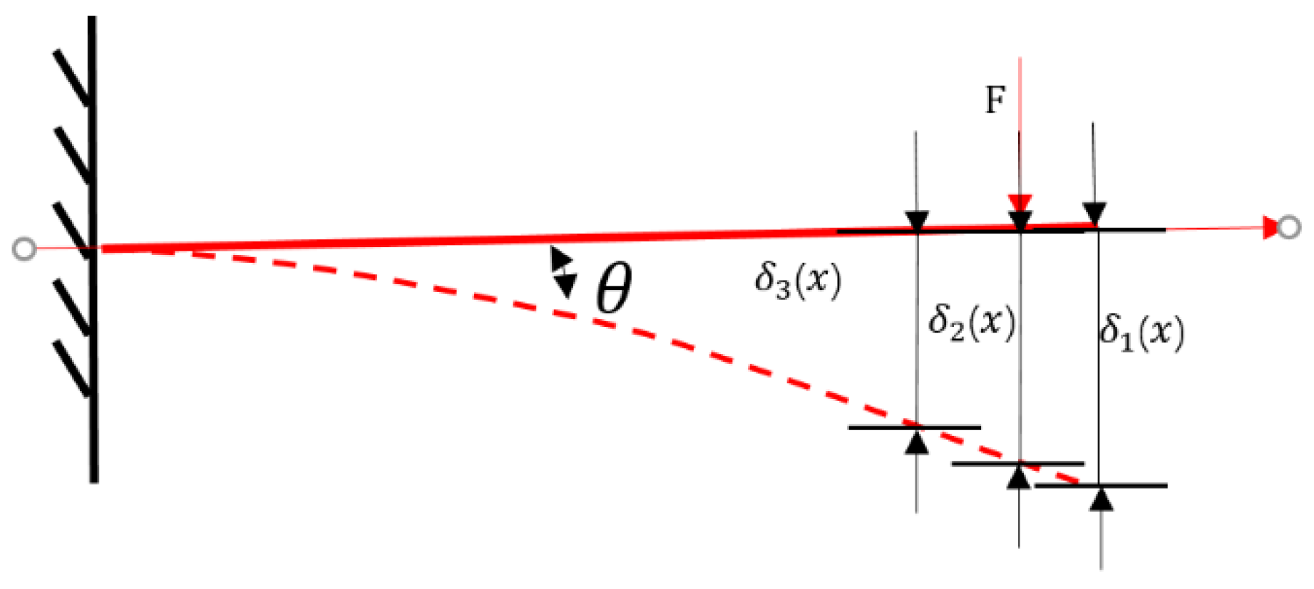
During cutting, the deflection caused by the cutting load is mainly extrusion deflection, torsional deflection, and bending deflection. Extrusion deflection is produced by the vertical component of the cutting load. Since the axial rigidity of a tool is relatively high, extrusion deflection can be ignored. In this paper, only bending deflection and torsional deflection caused by the horizontal component of the cutting load are analyzed (Figure 1). Under a cutting load, a tool deforms elastically, which satisfies the conditions of small deflection, Hooke’s law, and the superposition principle.
2.1.1. Theory of Tool Bending and Torsional Deflection
Under a cutting load, part of the edge of an end milling cutter has bending deflection and torsional deflection. The work of the cutting force is transformed into energy that is stored within the cutter, so that the cutter can perform external work. This energy is called elastic energy . The cutting load is the main cause of tool bending deflection, as shown in Figure 2 [20,21]. If the tool is small, there is a bending moment and torque due to the cutting force. Because the deflections caused by these two internal force components are independent of one another, the total strain energy is equal to the sum of the strain energies when they act alone:
where the strain energy is generated by the bending, and is produced by the torsion.
The empirical formula of the tool deflection is:
where is the cutting force, is the tool deflection under the cutting force, and and are natural constants. According to the formula of deflection, the relationship between tool deflection and cantilever length is cubic. For a tool of the same diameter, when the length of the cantilever is doubled, the deflection will increase by 8 times. The relationship between tool deflection and tool diameter is the fourth power. For a tool of the same length, when the diameter of the tool is reduced by 1 time, the deflection will increase by 16 times. In precision machining, the heat has a great influence on the small diameter and large cantilever tools. Therefore, periodic high-frequency loading deflection is formed. The energy consumed here can be calculated. The energy varies with the cutting force; the formula for calculating the energy is as follows:
A tool that deflects stores potential energy. When the deflection is released, the energy is released. If the angle between the front and back cutting edges is not 180°, friction is inevitable. Even if the process is elastic, the process is non-zero sum. The reaction force of tool deflection is consumed by friction before it can be loaded to the next cutting. Specifically, when the interval is 90°, the friction caused by the tool deflection is the greatest and the heat generated is the greatest. Because of the energy conservation, the potential energy is converted into internal energy and, finally, released in the form of heat. In the milling phase, the deflection energy of the tool accumulates as the milling forces increase. In the non-milling phase, the tool deflection energy is released.
2.1.2. Tool Potential Energy
The tool is affected by the cutting force and the work done in the direction of the cutting force. Therefore, the milling force and the tool deflection are the basic parameters needed to calculate the tool deflection energy. These can be obtained by experiments, ensuring that they are consistent. In the experiments, the acquisition system for the three-way force-measuring instrument has the same sampling frequency and time length as the displacement sensor.
- Cutting force
The magnitude of the cutting force determines the bending and torsional potential energy of the tool. The experiment was carried out on a QLM27100-5X five-axis linkage gantry (Figure 3, Nanjing, China). The cutting force was measured for different cutting parameters by a Kistler 9265B dynamic dynamometer. The spindle speed was 9000 r/min, the feed speed was 2000 mm/min, the axial milling depth was 3 mm, the radial milling depth was 0.5 mm, and the sampling frequency was 15,000 Hz. The workpiece material was 7075 aluminum alloy. A special, customized tool was used in the experiment. The tool material was cemented carbide. The tool parameters are shown in Table 1.
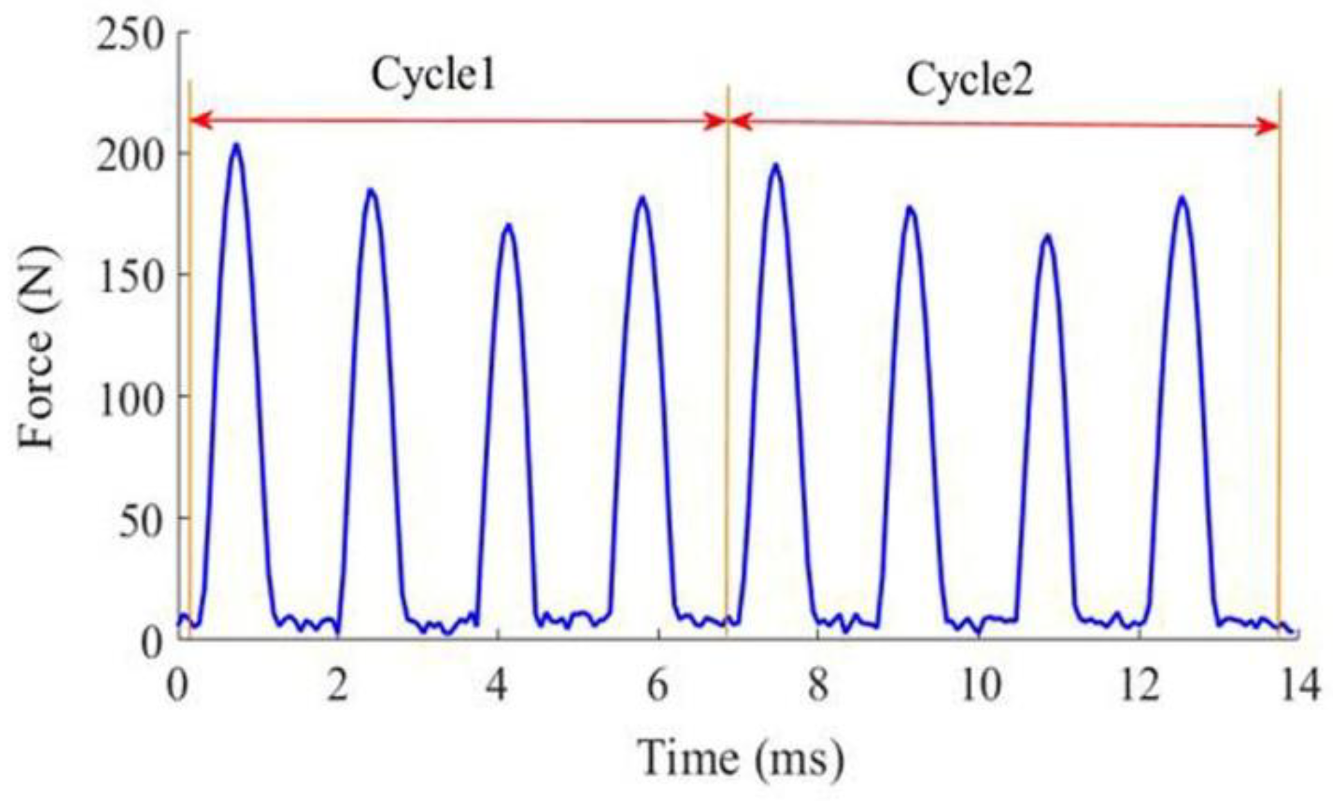
Because the side milling is intermittent, the milling cycle is classified into a cutting phase and a non-cutting phase. The milling force in the X and Y directions changes periodically. Moreover, the tool has four milling edges, so there are four peaks per cycle. The maximum milling force is 205 N (Figure 4). The data collected in this experiment were used to calculate the bending and torsional potential energy of the tool.
- 2.
- Tool deflection
The tool-tip displacement directly affects the tool deflection error. Based on non-contact measurements of eddy currents, the deflection of the tool is measured on-line. Two eddy current sensors measure the deflection of the tool in the X and Y directions. In this paper, the spiral blade diameter was 80% of the handle diameter. To ensure that the experimental data were true and practical, a special, customized cutting tool was used (Appendix A). The sampling frequency was set to 15,000 Hz. The experimental setup is shown in Figure 5. The comprehensive deflection was obtained by calculating the resultant displacement. In the end, the deflection of the tool tip was calculated by using the deflection formula of the cantilever beam.
The experiment in the graph reflects the displacement of the whole machining system. The purpose of this experiment is to obtain the tool deflection only under the action of cutting force. In order to minimize the impact of other factors, the experimental conditions must be limited when measuring displacement (Appendix A).
Figure 6 shows two cycles of the combined displacement of the four-edged tool in the X and Y directions under a milling force. The maximum displacement was ~0.18 mm. The errors were large, but the graph indicates the validity and authenticity of the deflection displacement data.
- 3.
- Calculation of tool potential energy
- (1)
- Potential energy under a milling force
From the milling force experiment, we obtained the resultant milling force on the tool (Figure 4). The first peak in the first cycle for the resultant force on the blade was used to calculate the bending and twisting potential energy of the cutter. As in Table 1, the tool diameter was 10 mm, the tool blade helix length was 30 mm, and the maximum overhang length of the cutter was 70 mm. The energy is calculated as:
From the above simplified calculation, the edge torsional energy of the end mill is 0.000034 J, which is much lower than the bending energy of 0.0652 J. Thus, the influence of the tool torsional deflection on the machining error can be ignored.
- (2)
- Calculation of potential energy by deflection
The displacement was measured experimentally as a metric for the tool deflection. The change rule of tool deflection was obtained through the tool displacement experiment. The tool deflection was the equivalent cantilever deflection. During the experiment, the sampling time and frequency of the cutting force were consistent with the frequency of the tool deflection. We used the peak of the first tooth displacement in the first cycle in Figure 6. Since the displacement was measured 15 mm from the tool tip, the displacement of the tool tip can be obtained as a linear proportion for a cantilever beam [21]:
this, from material mechanics:
- (3)
- Potential energy analysis
There must always be tool deflection energy; due to the existence of tool displacement, the milling forces in X and Y directions, and the deflection of X and Y tools, respectively, were obtained at different times. The tool potential energy was calculated using a combination of the force and the resultant force deflection, and experimental displacement data verified the measured potential energy.
During milling, the milling force changes periodically as the cutting tool moves in and out (Figure 4). The deflection energy of the cutter changes as the milling force changes. From the experimental data, we can obtain the energy for continuous milling with four cutter teeth, as shown in Figure 7. The maximum potential energy in the deflection of a cutter tooth is 0.065 J.
It is obvious from the results that the tool potential energy () obtained from the displacement is greater than the tool potential energy () calculated using the cutting force. This is because the tool displacement depends on other factors that also affect the tool deflection, such as vibration in the machine tool system, machine error, and clamping error. However, the tool deflection calculated using the cutting force is within a reasonable range.
2.2. Heat Generation
Take the four-fluted milling cutter as an example: the numbers of the four cutting edges are 1, 2, 3, and 4, respectively. When the #1 edge starts from the cut-in angle to the end of the cut-out angle, the cutter completes the loading and unloading. In the cutting process, the machining of a cutter tooth is divided into three parts [22]:
- Cutter edge cutting-in stage
The cutting force increases from 0 to the maximum at the beginning of cutting. The deflection energy of the tool due to the force is also increased to the maximum.
- 2.
- Cutter edge cutting-out stage
With the decrease in cutting forces, the deflection energy of the cutting tool also begins to decrease. At this time, the tool mainly transforms the reduced deflection energy into heat energy through friction until the tool cuts out. The force of the tool is reduced to 0, and the deflection energy is reduced to 0.
- 3.
- Cutter edge energy absorption process
After the cutting process of the cutting edge, the heat absorbed by friction is the greatest, and the temperature caused by the heat reaches its highest. At this point, the completed energy absorption process ends until the next tooth cutting process begins. Energy conversion follows this process in a cycle, as shown in Figure 8.
It can be reasonably assumed that the tool potential energy is finally converted to heat energy (considering anelasticity, friction, and vibration) [23], and is transformed by the contact zone between the tool tip and the workpiece in the form of friction [22,24]. The final result of this energy causes the tool temperature to rise. This phenomenon only exists during the cutting process; the deformation heat of the tool occupies a part of the friction heat, and conforms to the temperature rise characteristics of the friction heat. Hence, the temperature rise shown in Figure 8.
3. Tool Temperature Modeling
In the typical milling process, the bending and twisting potential energy of tool deflection is converted into heat energy, and the temperature model is established.
3.1. Numerical Methodology
At present, the common numerical methods for solving heat conduction equations include the finite element method, finite difference method, and finite volume method. As far as the discrete method is concerned, the finite element method is the change rule of the assumed value between the mesh points (the interpolation function), and takes it as the approximate solution. The finite difference method only takes the numerical values of the grid points into account, without considering how the values change between the mesh points. The finite volume method can be regarded as the intermediate between the finite element method and the finite difference method. The implementation process of the finite volume method is as follows: Firstly, the required solution region is divided into adjacent but non-overlapping control bodies, and then the corresponding nodes are used to represent each control body. Finally, the discrete equation is derived by integrating the conservative control equation with the control volume.
According to the structure of the control volume and the difference in variable storage, the finite volume method is divided into two types: the cell-centered finite volume method, and the cell-vertex finite volume method. The cell-centered finite volume method constructs the control volume around the nodes, and the variables to be solved are defined on the mesh nodes, so it is not suitable for arbitrary polygon meshes. The control volume of the cell-vertex finite volume method is the mesh element, and the variables to be solved are defined in the center of the element. In this paper, the cell-centered finite volume method is used to solve the problem.
3.2. Heat Conduction Equation
Heat transfer analysis should finally be focused on the milling cutter itself, as its thermal behavior directly makes a great impact on the machining error of the machine tool and cutter system. In order to obtain the temperature distribution of the milling cutter, the finite volume method is used to solve the three-dimensional heat conduction problem.
The integral form is used to describe the governing equation of heat conduction. The heat transfer equation is:
Because of the complexity of the volume integral, Gauss’s theorem is used to transform the volume integral into an area integral.
Gauss’s theorem can be written as follows:
where is ρ is the density, c is the heat capacity, k is the thermal conductivity, and is the convective heat transfer coefficient.
3.3. Numerical Discretization and Boundary Conditions
3.3.1. Numerical Discretization
The numerical discretization and application of the boundary conditions are necessary for solving the solid heat conduction. The control volume is a layered mesh element discretized from the computational domain, and the variables are stored in the cell center. Variables and physical parameters are defined in the center of the element, and are assumed to be uniformly distributed in the element.
The equation of heat conduction (Equation (6)) can be discretized as follows:
where the subscript represents the center of the current element , the subscript represents the center of the adjacent element , is the temperature at the center of the current element , and is the temperature at the center of the adjacent element , the subscript represents the element face, is the time step, the superscripts and represent the current time and the previous time, respectively, the initial temperature field is given according to the actual situation, is the area vector of the element surface , and is the distance vector across the faces between elements.
For heat conduction, there are three kinds of the boundary conditions. The first kind is the given temperature:
The second kind of boundary condition is the given heat flow:
The third kind of boundary condition, also known as the mixed boundary condition, is the given ambient temperature and heat transfer coefficient:
where is the temperature on boundary , is the normal heat flux on boundary , is the convection heat transfer coefficient on boundary , and is the ambient temperature. Subscript B represents the boundary.
To find the boundary conditions for heat conduction, Equation (2) can be discretized as follows:
where is the number of inner face elements, superscript is the number of element faces of the second type on boundary , superscript is the number of element faces of the third type on boundary , is the component of the external normal unit vector n perpendicular to interface S, is the boundary temperature, and is the normal heat flux given on the boundary. The other terms are the same as in Equation (10).
The tool edge is subdivided into a series of equivalent layers. A hexahedral finite volume mesh is used. To facilitate the division of the finite volume mesh, the section of the four-edged milling cutter perpendicular to its axis is reasonably simplified using the unstructured adaptive mesh division technique. When the mesh is divided from a central point to the outside, the mesh encryption technique based on the equal difference sequence is adopted. Figure 9 shows the encrypted point layer. The lower vertex coordinates of the hexahedral mesh are stretched in the positive Z direction and rotated along the tilt direction of the edge in order to obtain the upper vertex, and then all of the vertex coordinates of the finite body mesh are obtained, so as to realize the division of the finite volume mesh.
3.3.2. Boundary Condition Analysis
Because the cutter has four cutting edges, the cutting is discontinuous. To simplify the calculations and reduce the computation time, the tool used in this model is considered to have only one cutting edge, as shown in Figure 10. The boundary conditions depend on whether or not the tooth is in contact with the workpiece.
The boundaries are shown in Figure 10. Boundary assumptions are as follows:
- Boundaries a and b: a is the front face and b is the back face of the milling cutter edge. In the range 0–3 mm in the Z direction of the cutter, boundaries a and b are endothermic during cutting and exothermic during non-cutting. The range 3–12 mm in the Z direction of the cutter does not participate in cutting, and is always exothermic.
- Boundaries c and f: During cutting, these are always in an exothermic state.
- Boundaries d and e: Since edge d is in contact with edge e, and far away from the tool nose, there is only a small amount of heat. Similarly, edge e sees only a small amount of heat. The heat and the emission are equal, so it is assumed that the boundary is adiabatic.
3.4. Heat Distribution
The potential energy in tool deflection is consumed by the friction between the front tool surface and the cutting surface (the first deflection area), and by the friction between the back tool surface and the surface of the workpiece being processed (the second deflection area). The friction converts the energy into heat, which causes the temperature to rise.
Casto et al. [25] researched the cutting heat distribution ratio. The workpiece material was AISI 1040, a carbide tool was used, the cutting speed was 99–240 m/min, and the rate of heat into the tool was 25–56%. When the workpiece material was AISI 4140, the tool was cemented carbide, and the cutting speed was 6–1200 m/min, Abukhshim et al. [26] verified that the proportion of heat into the tool was 15–60%. Similarly, Mabrouki et al. [27] proved that the rate of heat into the tool was 65% when the workpiece material was AISI 4340, a carbide tool was used, and the cutting speed was 100 m/min. From the various literature, the equivalent cutting heat for aluminum alloys at different cutting speeds is 15–65%. Here, the average value of 30% is taken as the equivalent heat.
The tool potential energy causes the temperature to rise due to the dissipation of friction energy, which can be represented by the transient thermal structure coupling model by including the effects of transients on thermal freedom. Two factors are needed: the ratio of the tool deflection potential energy converted into heat by friction consumption is ; and the coefficient for heat distribution between
the workpiece, the chips, and the tool is h.
The tool deflection potential energy consumed by friction [28] is defined as:
where is the equivalent friction stress and is the sliding rate. Moreover:
where is the tool deflection potential energy dissipated by friction on the tool surface, is the tool deflection potential energy dissipated by friction on the chip contact surface, and is the tool deflection potential energy consumed by friction on the workpiece contact surface.
For tool energy:
and:
where subscript t represents the tool, subscript c represents the chip, and subscript w represents the workpiece. Subscript represents the front tool face and subscript represents the back tool face.
When the tool potential energy is being consumed, the effective contact surface between the front tool surface and chip is relatively small. Moreover, the area of the back tool surface is relatively small compared with the surface area being cut. The heat absorbed by the front and back faces of the tool is equivalent to 1/3 of the total deflection potential energy of the tool, namely:
The tool deflection energy is described in Equation (3). The parameters can be obtained through experiments.
4. Numerical Simulation
4.1. Simulation Parameters and Programming Flow
To verify the temperature model proposed in Section 3, the prediction temperature field of the tool is obtained via programming in MATLAB. The processing parameters are the same as those in Section 2.1.2. The tool parameters are shown in Table 1. In order to reduce the difficulty of analyzing the temperature model, the arc spiral groove is simplified to a V-groove, and the experimental results show that the deviation is acceptable. The programming flow chart is shown in Figure 11.
4.2. Numerical Analysis
Figure 12 is the three-dimensional temperature distribution of different positions of the tool edge over time; it shows the temperature of one cutting edge as it varies by the cutting depth of the tool for 250 cycles. The axial cutting depth of the tool was 3 mm. The temperature of the cutting edge varied with the cutting depth of the tool. The temperature in the vicinity of the tool tip was relatively high, and along the axial of the tool, the temperature at the tip of the tool decreased significantly at 3 mm. The temperature of the part of the cutting edge that was not involved in cutting was low, dropping to room temperature (20 °C).
The peak temperature rose from 22.7 °C to 24.9 °C, and the minimum temperature rose from 20.4 °C to 22.3 °C, over 250 consecutive cycles (Figure 13).
Through a reasonable optimization of the mesh and boundary conditions, an isothermal distribution for the cutter tooth was obtained via numerical simulation. The refinement of the mesh layer and step size depended on the importance of the position within the tooth. Figure 14 displays the temperature distribution of the front, back, and nose of the blade involved in milling. The temperature of the cutter tooth increased from 20 °C to 25 °C over 250 cycles.
5. Experiments
It is difficult to verify the temperature rise caused by the tool deflection; in this paper, separation experiments are conducted for further research. Sato et al. [29] described the cyclic temperature variation beneath the rake face of a cutting tool in end milling. In this study, a new technique in radiation temperature measurement using two optical fibers was applied to investigate the temperature variation at different depths in a tool insert during the cutting and non-cutting cycles in end milling. The aim of the experiments was to separate the cutting friction heat from the tool deflection energy. During the experiments, the experimental parameters were the same as the simulation parameters in Section 4.1. The experiments were carried out on a QLM27100-5X five-axis linkage gantry (Qiaolian, Wuxi, China). The temperature was measured with an Optris PI200, PI450 (Optris, Germany), and infrared temperature instrument, and the measuring position was 4 mm away from the tool tip.
5.1. Total Temperature Rise of the Cutting Tool
Based on the above conditions, milling experiments were carried out with a gantry machine tool. The lens of the infrared thermal imager was fixed, and the rectangular coordinates of the measuring area were aligned to the measuring position. The experimental setup is shown in Figure 15.
5.2. Temperature Rise Due to Tool Friction Alone
The experimental setup to measure the temperature rise due to friction is shown in Figure 16. A dynamic friction block (1) was connected to a force generator. Component (2) refers to the static friction block, which was fixed on the machine tool and 10 μm away from the mandrel (3). The cambered surfaces were made on the static friction block (4) and dynamic friction block (5), respectively, each arc angle was 60°, and the radius of the arcs was the same as the mandrel radius.
In order to generate friction heat between the dynamic friction block and the rotating mandrel, the force generator needed to apply the same size and frequency load to the dynamic friction block. The temperature was measured at a height of 4 mm. This temperature rise was caused by tool friction alone.
5.3. Temperature Rise Due to Tool Deflection and Friction
The experimental device for measuring the temperature rise on account of deflection and friction of an equivalent tool (mandrel) under a simulated cutting load is shown in Figure 17. The experimental equipment includes a powerful generator, a machine tool spindle, a mandrel, a workpiece, a machine tool workbench, an L-shaped base plate, a support guide rail, a force sensor, and an infrared thermometer. A 3-mm-deep groove was cut into the workpiece. The radius of the top arc was 5 mm. This was in contact with the side surface of the mandrel, which had a diameter of 10 mm.
5.4. Results and Discussion
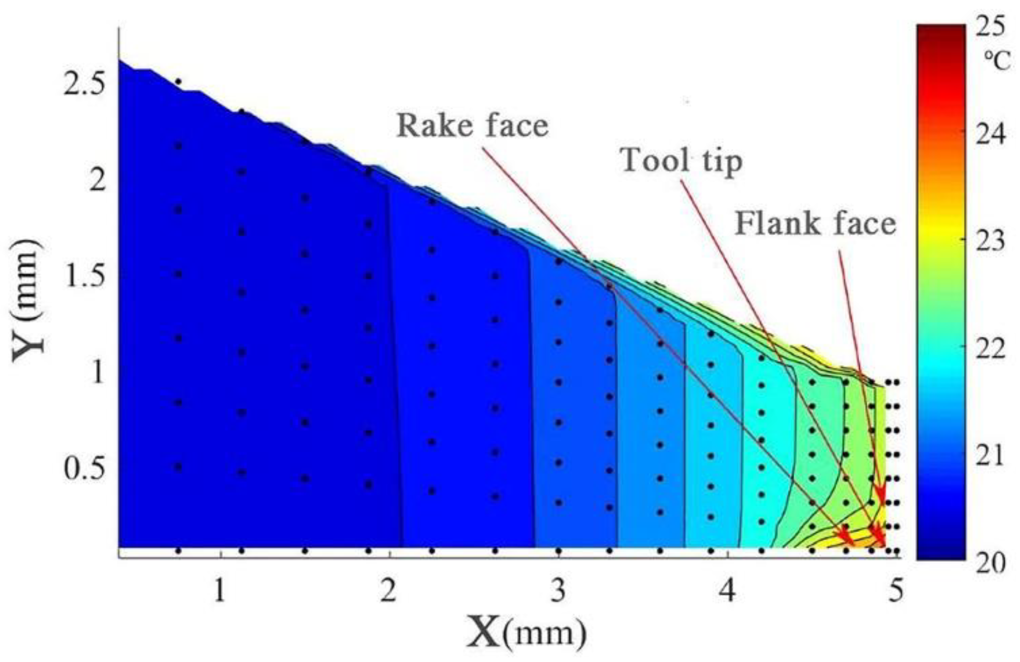
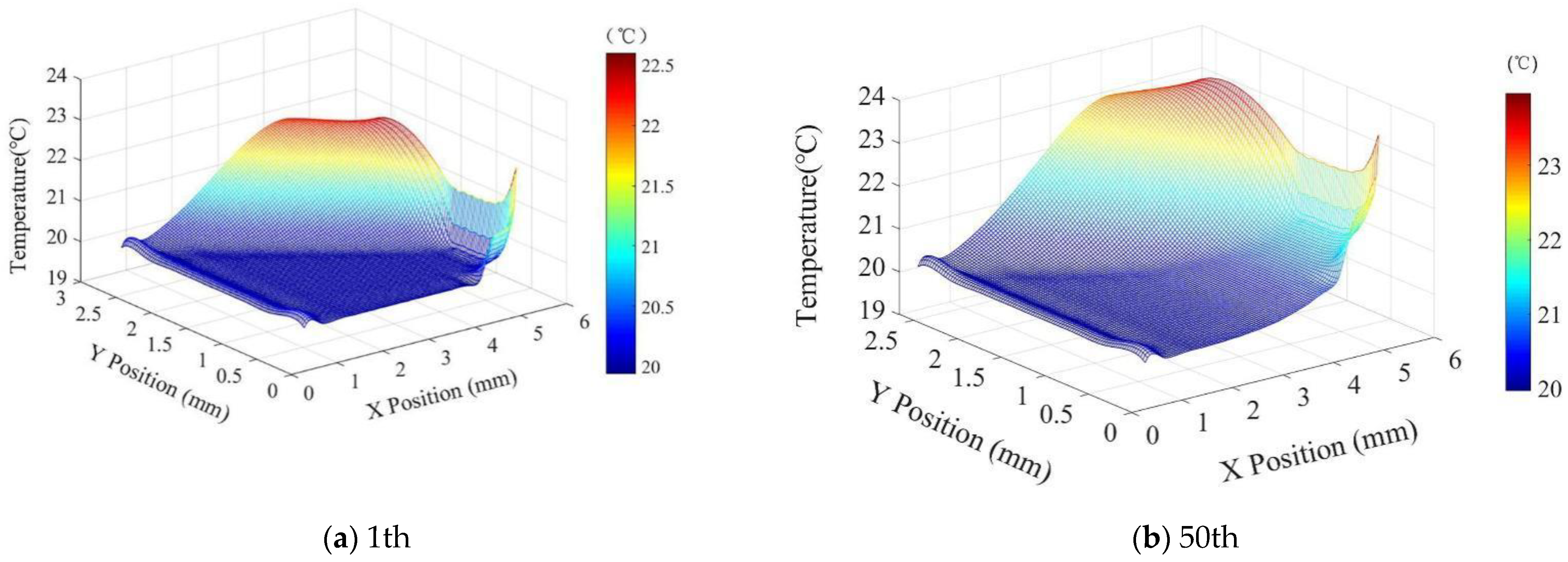
In Section 4.1, the results of tool temperature rise were obtained via MATLAB programming. Figure 18a–d shows the three-dimensional temperature distribution of the X–Y direction section of the tool nose, obtained via the numerical model, when the highest temperature is reached in the 1st, 50th, 150th, and 250th cuttings, respectively. Figure 19a–d shows the corresponding temperature gradient distribution. It can be seen that the high-temperature region is mainly concentrated in the range near the tool nose, which is also the range with the largest temperature gradient. The temperature of the tool nose region increases with the increased milling time, and gradually decreases outward along the tool tip.
Figure 19 shows that the highest temperature is on the tool flank, rather than at the tool nose. There are two reasons for this: Firstly, the mechanism of heat generation is the tool deflection caused by the force. In Section 3.4, the energy was equivalent to three equal parts. However, in finish machining, the chips are smaller, and the contact surface with the rake face is smaller. The contact area between the tool flank and the workpiece is larger, and the force on the flank is also larger. Therefore, the temperature of the flank is high. Secondly, variables of the finite volume of the lattice center are located in the center of the element, which may have a small deviation from the tool tip.
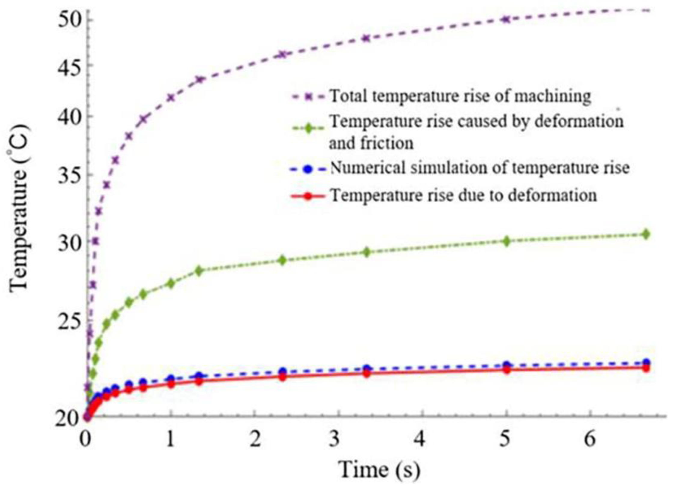
The differences in the temperatures measured in Section 5.2 and Section 5.3 are the temperature rise due to the transformation of friction into tool potential energy. In order to express this more intuitively, the predictive and experimental values of the temperature are plotted as curves in Figure 20. The temperature measured in the tool deflection experiment (red curve) is consistent with that of the numerical simulation (blue curve). However, the simulation results tend to be higher than the experimental results. It may be hypothesized that the temperature rise caused by tool deflection is relatively small compared with that caused by the environment and heat loss. The ratio of the experimental value for the tool deflection temperature rise to the total cutting temperature rise is up to 6.57%. Based on the distinct mechanism of the heat source, the heat effect of the heat source on the front and back faces is different from that of other heat sources [14,30].
6. Conclusions
In this paper, a new heat source that caused the thermal error of the cutting tools was proposed, and was verified by the numerical simulations and experiments. The potential energies of the tool bending and torsion were analyzed. The results were verified in two different ways. Based on the analysis and experimental results, the following conclusions can be drawn:
- (1)
- A heat generation mechanism is proposed. In precision or micro milling, heat has a great influence on a tool with small diameter and large cantilever elongation.
- (2)
- For the cutting parameters used, the change rule in the cutting force and cutter deflection is consistent with the change in the tool potential energy. The torsional potential energy of the tool is much less than its bending potential energy. Compared with the two-dimensional simulation, the boundary conditions for tool heat conduction can be set more accurately using the finite volume method. Moreover, the numerical discretization is more reasonable, and the calculation results are more realistic.
- (3)
- A numerical calculation based on the working conditions used shows that the high-temperature region is mainly concentrated in the range near the tool nose, and the highest temperature is on the back face.
- (4)
- A test platform to measure the tool temperature rise caused by the tool deflection was designed. The relative difference between the temperature calculated and the measured temperature was less than 5%. In addition, the temperature rise due to the tool deflection potential energy was consistent with the temperature rise during cutting, and was up to 6.57% of the total temperature rise of the cutting tool.
This method has a specific reference value for the research of cutting and friction, and can be extended to related thermal fields. However, further exploration and improvement are needed in the experimental application.
Author Contributions
Conceptualization, W.Y.; methodology, W.Y.; software, Y.G.; validation, X.X.; formal analysis, W.Y.; investigation, Y.G.; resources, Y.G.; data curation, X.X.; writing—original draft preparation, Y.G.; writing—review and editing, W.Y.; supervision, W.Y.; project administration, Y.G. All authors have read and agreed to the published version of the manuscript.
Funding
This work was financially supported by the National Natural Science Foundation of China (No. 51775277, 51575272).
Institutional Review Board Statement
Not applicable.
Informed Consent Statement
Not applicable.
Conflicts of Interest
The authors declare no conflict of interest.
Nomenclature
| Density, (kg/m3) | |
| C | Specific heat, J/(kg·K) |
| K | Thermal conductivity, W/(m·K) |
| Heat flux, W/mm2 | |
| Current element, mm3 | |
| The f-th adjacent element, mm3 | |
| Temperature at the center ofthe current element , °C | |
| Temperature at the center ofthe adjacent element , °C | |
| A | Area vector of the elementSurface , mm2 |
| e | Distance vector across thefaces between elements, mm |
| Time step | |
| Current time, s | |
| Previous time, s | |
| the number of inner face elements | |
| Temperature on boundary, °C | |
| Normal heat flux on boundary, W/mm2 | |
| Thermal conductivity on boundary , W/(m K) | |
| Component of the external normal unit vector n perpendicular to interface S | |
| the number of element faces of the second type on boundary | |
| the number of element faces of the third type on boundary |
Appendix A
- 1
- To ensure that the experimental data were true and practical, a special customized cutting tool was used. A ring with a radius of 15 mm was placed around the tool 15 mm away from the tip and welded in place. The tool and the ring were concentric. The customized tool had two functions: First, it prevented interference between the two eddy current displacement sensors. Second, the cross-sections of the blade and the tip were the same, so that the displacement of the blade truly reflected the displacement of the tip.
- 2
- In order to minimize the impact of other factors, we had to limit the experimental conditions when measuring displacement:
- (1)
- The experiment was executed under cold machine conditions in order to diminish the influence of thermal error of machine tool.
- (2)
- In the experiment, it was necessary to monitor the vibration signal, reduce the vibration, and ensure the stability of milling.
- (3)
- The displacement information of no-load and load cutting should be measured simultaneously under the same conditions.
- 3
- In the manuscript, the cell-centered finite volume method was used. The control volume was usually a mesh element discretion from the computational domain, and the dependent variables were stored in the center of the cell. Any unstructured mesh was used to divide the computational domain, and the mesh element was used as the control equation of heat dissipation.
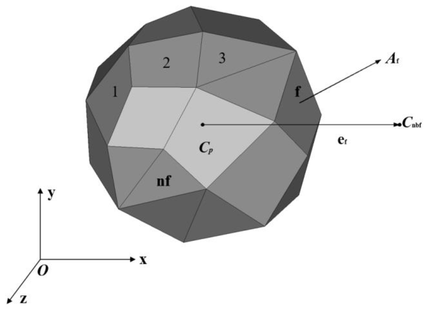
All variables and physical parameters were defined in the center of the element, and were assumed to be uniformly distributed in the element. Figure A1 is a schematic diagram of any mesh element in a Cartesian coordinate system. It is surrounded by units. is the current element, is the f-th (f = 1, 2, 3, … nf) adjacent element, and the distance vector of the unit center is . is the area vector of unit surface f. Along the outer normal direction, the modulus is equal to the area of the unit surface.
Figure A1.
Control volume of cell-centered finite volume method.
References
- Bi, Y.B.; Fang, Q.; Dong, Y.H.; Ke, Y.L. Research on 3D numerical simulation and experiment of cutting temperature for high speed milling of aerospace aluminum alloy. Chin. J. Mech. Eng. 2010, 46, 160–165. [Google Scholar] [CrossRef]
- Wan, M.; Zhang, W.H. Systematic study on cutting force modelling methods for peripherailling. Int. J. Mach. Tool Manuf. 2009, 49, 424–432. [Google Scholar] [CrossRef]
- Budak, E.; Altintas, Y. Modeling and avoidance of static form errors in peripheral milling of plates. Int. J. Mach. Tool Manuf. 1995, 35, 459–476. [Google Scholar] [CrossRef]
- Dotcheva, M.; Millward, H.; Lewis, A. The evaluation of cutting-force coefficients using surface error measurements. J. Mater. Process. Technol. 2008, 196, 42–51. [Google Scholar] [CrossRef]
- Colpani, A.; Fiorentino, A.; Ceretti, E.; Attanasio, A. Tool wear analysis in micromilling of titanium alloy. Precis. Eng. 2019, 57, 83–94. [Google Scholar] [CrossRef]
- Shaw, M.C. Metal Cutting Principles, 2nd ed.; Oxford University Press: Oxford, UK, 2005; pp. 9–12. [Google Scholar]
- Levin, P. A general solutions of 3-D quasi-steady-state problem of a moving heat source on a semi-infinite solid. Mech. Res. Commun. 2008, 353, 151–157. [Google Scholar] [CrossRef]
- Xu, H.; Chen, W.W.; Zhou, K.; Huang, Y.; Wang, Q.J. Temperature field computation for a rotating cylindrical workpiece under laser quenching. Int. J. Adv. Manuf. Tech. 2010, 47, 679–686. [Google Scholar] [CrossRef]
- Wang, Z. Study on the Temperature Field Modelling and the Real-Time Online Temperature Measuring Technique for the High Speed End Mill. Ph.D. Thesis, Harbin University of Science and Technology, Harbin, China, 2015. [Google Scholar]
- Putz, M.; Schmidt, G.; Semmler, U.; Dix, M.; Bräunig, M.; Brockmann, M.; Gierlings, S. Heat Flux in Cutting: Importance, Simulation and Validation. Procedia CIRP 2015, 31, 334–339. [Google Scholar] [CrossRef]
- Wu, B.H.; Cui, D.; He, X.D.; Zhang, D.H.; Kai, K. Cutting tool temperature prediction method using analytical model for end milling. Chin. J. Aeronaut. 2016, 29, 1788–1794. [Google Scholar]
- Wu, X.; Li, J.; Jin, Y.; Zheng, S. Temperature calculation of the tool and chip in slicing process with equal-rake angle arc-tooth slice tool. Mech. Syst. Signal Process. 2020, 143, 106793. [Google Scholar] [CrossRef]
- Islam, C.; Altintas, Y. A two-dimensional transient thermal model for coated cutting tools. Trans. ASME J. Manuf. Sci. Eng. 2019, 141, 071003–071014. [Google Scholar] [CrossRef]
- Shan, C.; Zhang, X.; Shen, B.; Zhang, D. An improved analytical model of cutting temperature in orthogonal cutting of Ti6Al4V. Chin. J. Aeronaut. 2019, 32, 759–769. [Google Scholar] [CrossRef]
- Reznikov, A.N. Thermophysical aspects of metal cutting processes. Mashinostroenie Mosc. 1981, 212. [Google Scholar]
- Kato, T.; Fujii, H. Temperature measurement of workpieces in converntional surface grinding. J. Manuf. Sci. 1998, 122, 297–303. [Google Scholar] [CrossRef]
- Rech, J.; Arrazola, P.J.; Claudin, C.; Courbon, C.; Pusavec, F.; Kopac, J. Characterisation of friction and heat partition coefficients at the tool-work material interface in cutting. CIRP Ann. 2013, 62, 79–82. [Google Scholar] [CrossRef]
- Gecim, B.; Winer, W.O. Transient temperatures in the vicinity of an asperity contact. ASME J. Tribol. 1985, 107, 333–342. [Google Scholar] [CrossRef]
- Zhao, J.F.; Liu, Z.Q. Modelling for prediction of time-varying heat partition coefficient at coated tool-chip interface in continuous turning and interrupted milling. Int. J. Mach. Tool Manuf. 2019, 147, 103467. [Google Scholar] [CrossRef]
- Liu, H.W. Mechanics of Materials. I, 4th ed.; Higher Education Press: Beijing, China, 2011; pp. 175–189. [Google Scholar]
- Liu, H.W. Mechanics of Materials. II, 4th ed.; Higher Education Press: Beijing, China, 2011; pp. 28–34. [Google Scholar]
- Chen, M.; An, Q.L.; Liu, Z.Q. Fundamentals and Applications of High Speed Cutting, 1st ed.; Shanghai Science and Technology Press: Shanghai, China, 2012. [Google Scholar]
- Zener, C. Elasticity and Anelasticity of the Metals; Science Press: Beijing, China, 1965. [Google Scholar]
- Jiang, F.L. Investigation of Transient Cutting Temperature of Workpiece and Cutting Tool in High Speed Intermittent Machining Process. Ph.D. Thesis, Shandong University, China, 2011. [Google Scholar]
- Casto, S.L.; Valvo, E.L.; Micari, F. Measurement of temperature distribution within tool in metal cutting experimental tests and numerical analysis. J. Mech. Sci. Technol. 1989, 20, 35–46. [Google Scholar] [CrossRef]
- Abukhshim, N.A.; Mativenga, P.T.; Sheikh, M.A. Investigation of heat partition in high speed turning of high strength alloy steel. Int. J. Mach. Tool Manuf. 2005, 45, 1687–1695. [Google Scholar] [CrossRef]
- Mabrouki, T.; Rigal, J.F. A contribution to a qualitative understanding of thermo-mechanical effects during chip formation in hard turning. J. Mater. Process. Technol. 2006, 176, 214–221. [Google Scholar] [CrossRef]
- Zhang, H.C. Ansys14.0 Theory Analysis and Engineering Application Example, 1st ed.; Machinery Industry Press: Beijing, China, 2012; p. 282. [Google Scholar]
- Sato, M.; Tamura, N.; Tanaka, H. Temperature Variation in the Cutting Tool in End Milling. ASME. J. Manuf. Sci. Eng. 2011, 133, 021005. [Google Scholar] [CrossRef]
- Shimanuki, K.J.; Hosokawa, A.; Koyano, T.; Furumoto, T.; Hashimoto, Y. Studies on high-efficiency and high-precision orthogonal turn-milling-The effects of relative cutting speed and tool axis offset on tool flank temperature. Precis Eng. 2020, 66, 180–187. [Google Scholar] [CrossRef]
Figure 1.
Bending and torsional deflection of a tool.
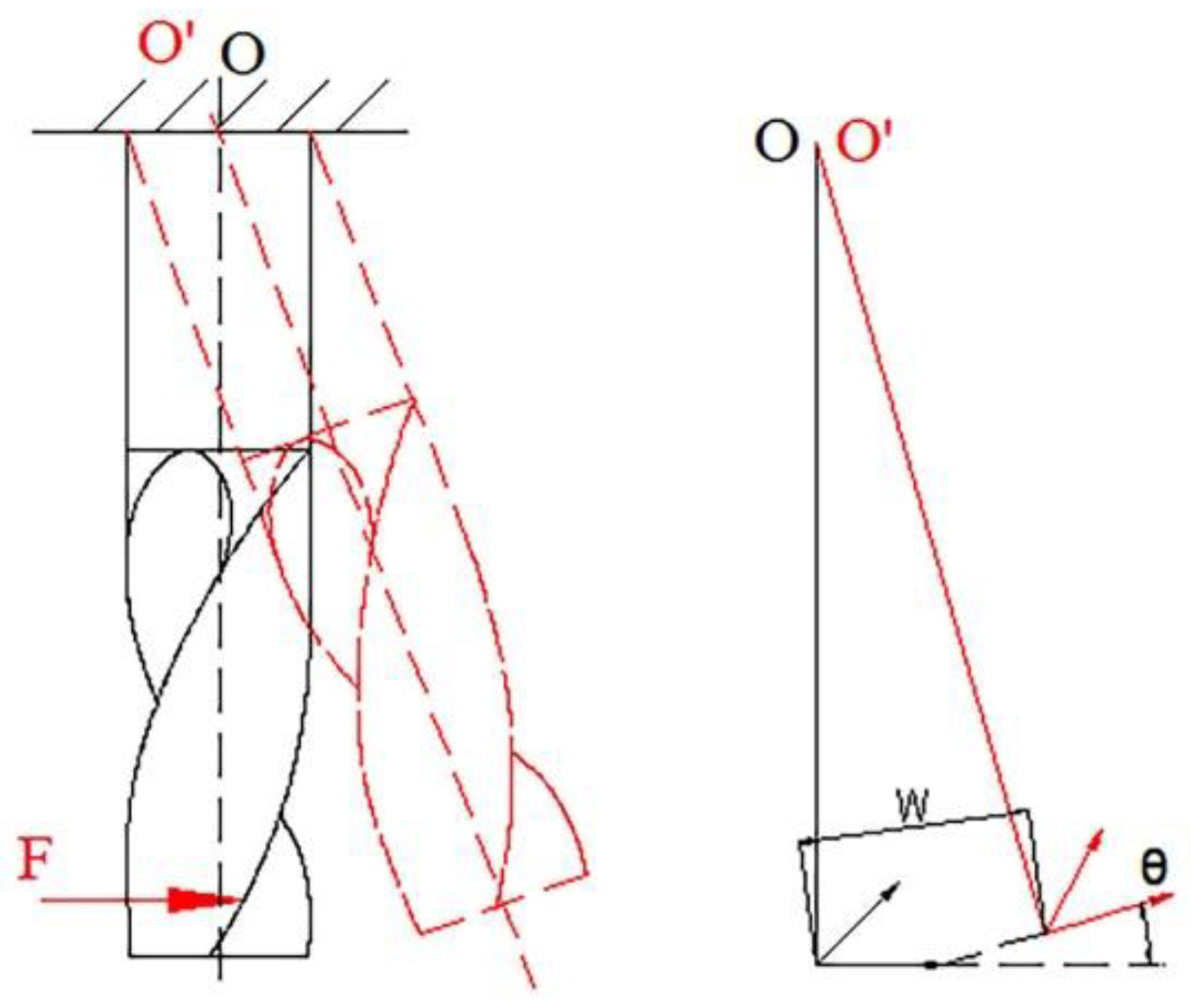
Figure 2.
Tool bending deflection.

Figure 3.
QLM27100-5X machine tool.
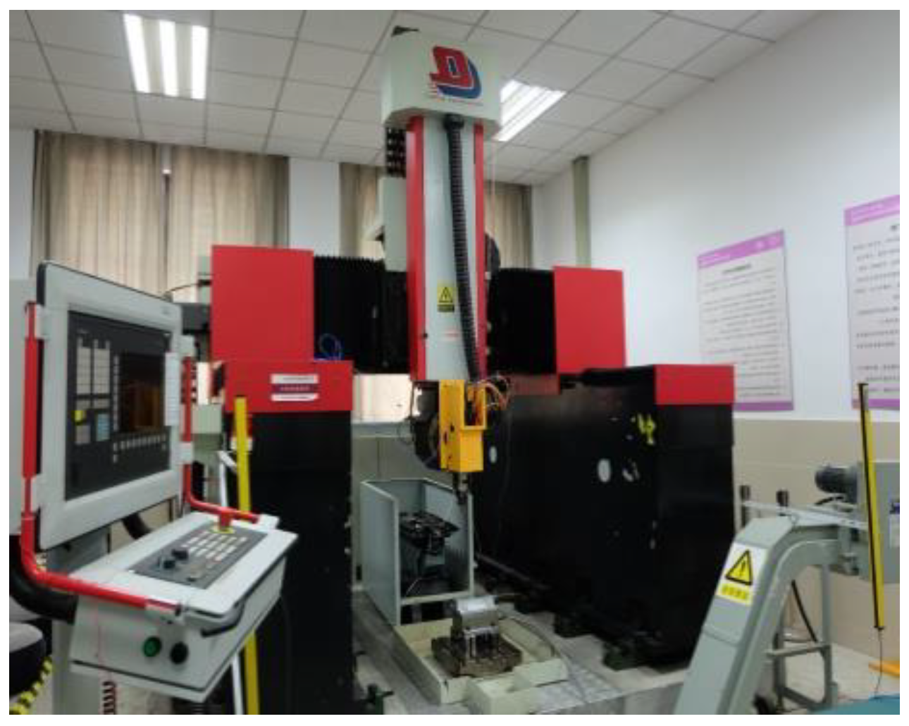
Figure 4.
Cycles of the resultant force on the tool in the X and Y directions.

Figure 5.
Photographs of the experimental setup for making on-line measurements of milling cutter deflection.
Figure 5.
Photographs of the experimental setup for making on-line measurements of milling cutter deflection.
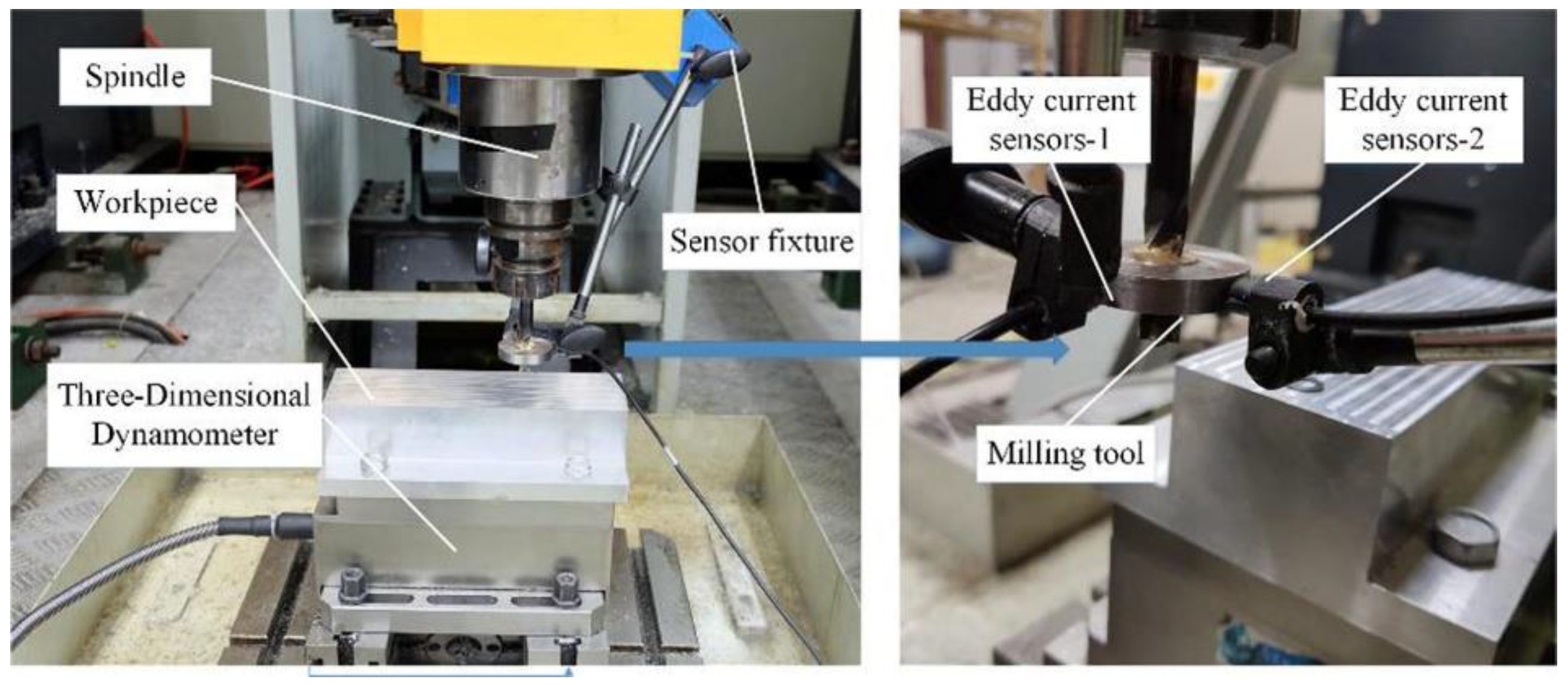
Figure 6.
Cycles of the combined displacement of the cutter in the X and Y directions.
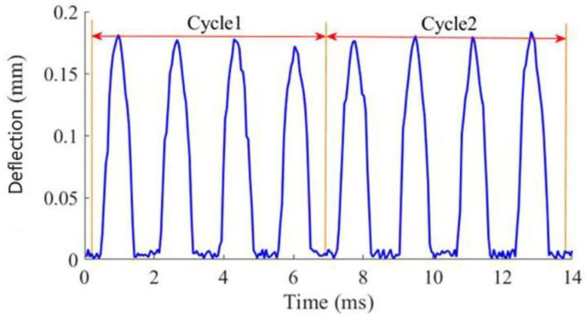
Figure 7.
Periodic variation of potential energy for tooth deflection.
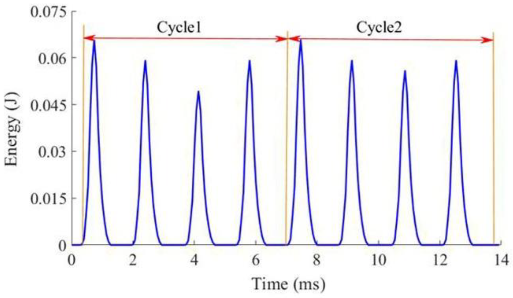
Figure 8.
Left: Tool showing the four teeth. Right: Energy changes in the edges during cutting.
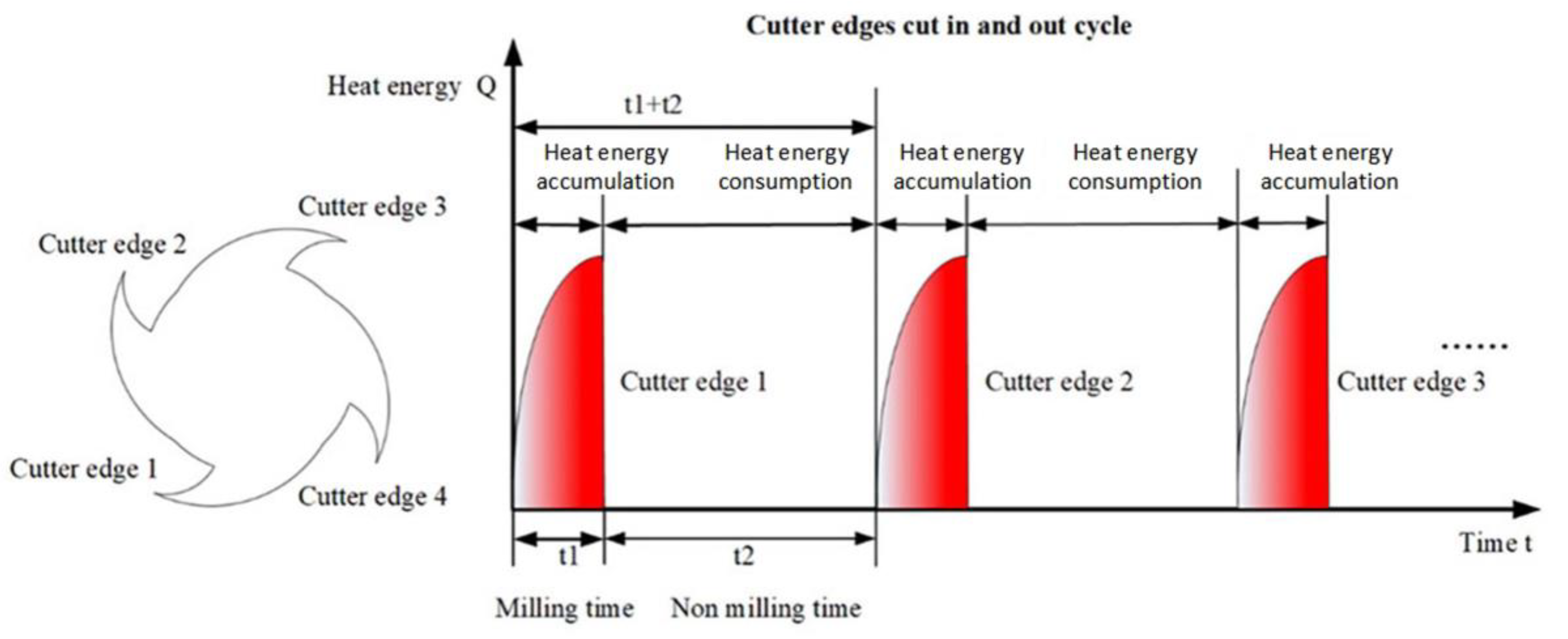
Figure 9.
Simplified section of the four-edged milling cutter perpendicular to its axis.

Figure 10.
The boundaries of a tooth.

Figure 11.
Flowchart for temperature rise calculation.
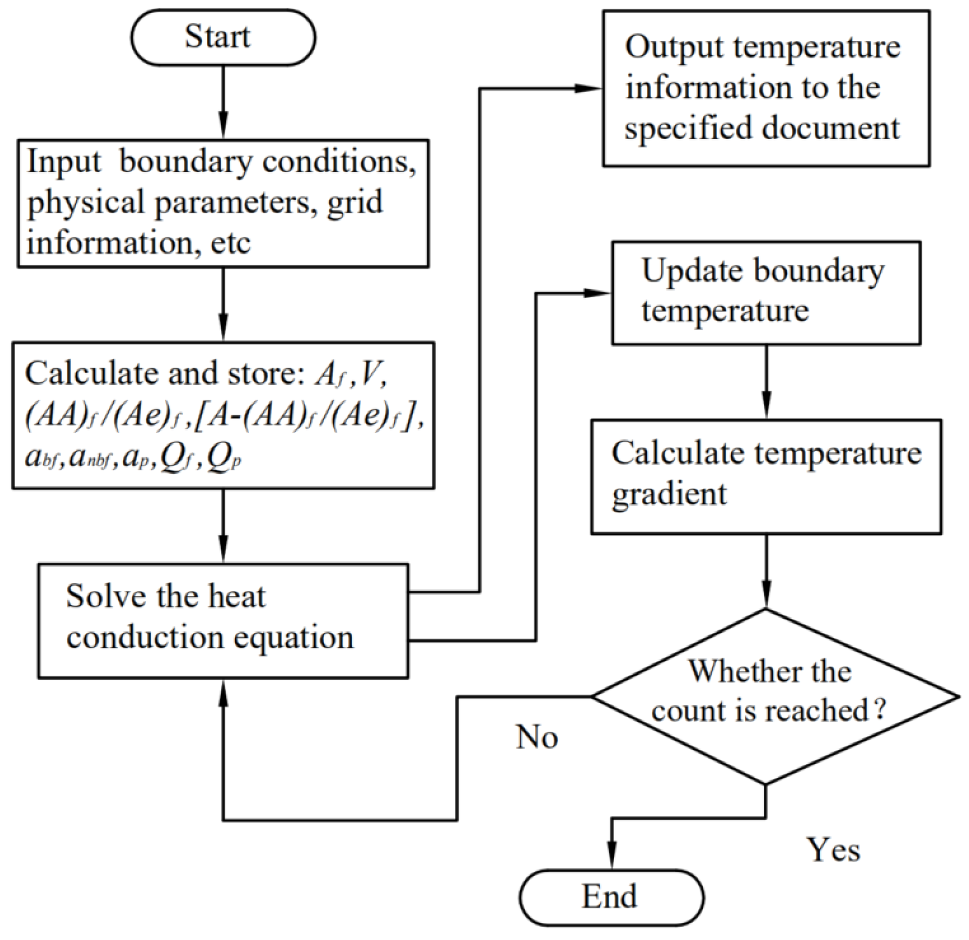
Figure 12.
3D temperature distribution of different positions of the tool edge with time.

Figure 13.
Temperature rise curve of the highest and lowest temperatures at the tip.
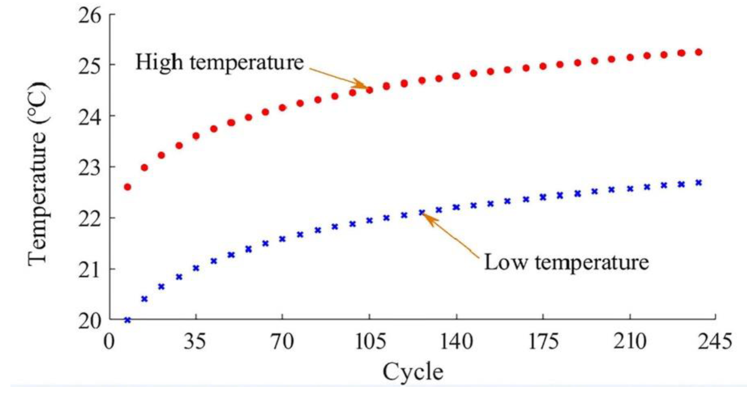
Figure 14.
Isothermal curve distribution of the cutting edge.

Figure 15.
Photograph of the setup for measuring the tool temperature during machining.
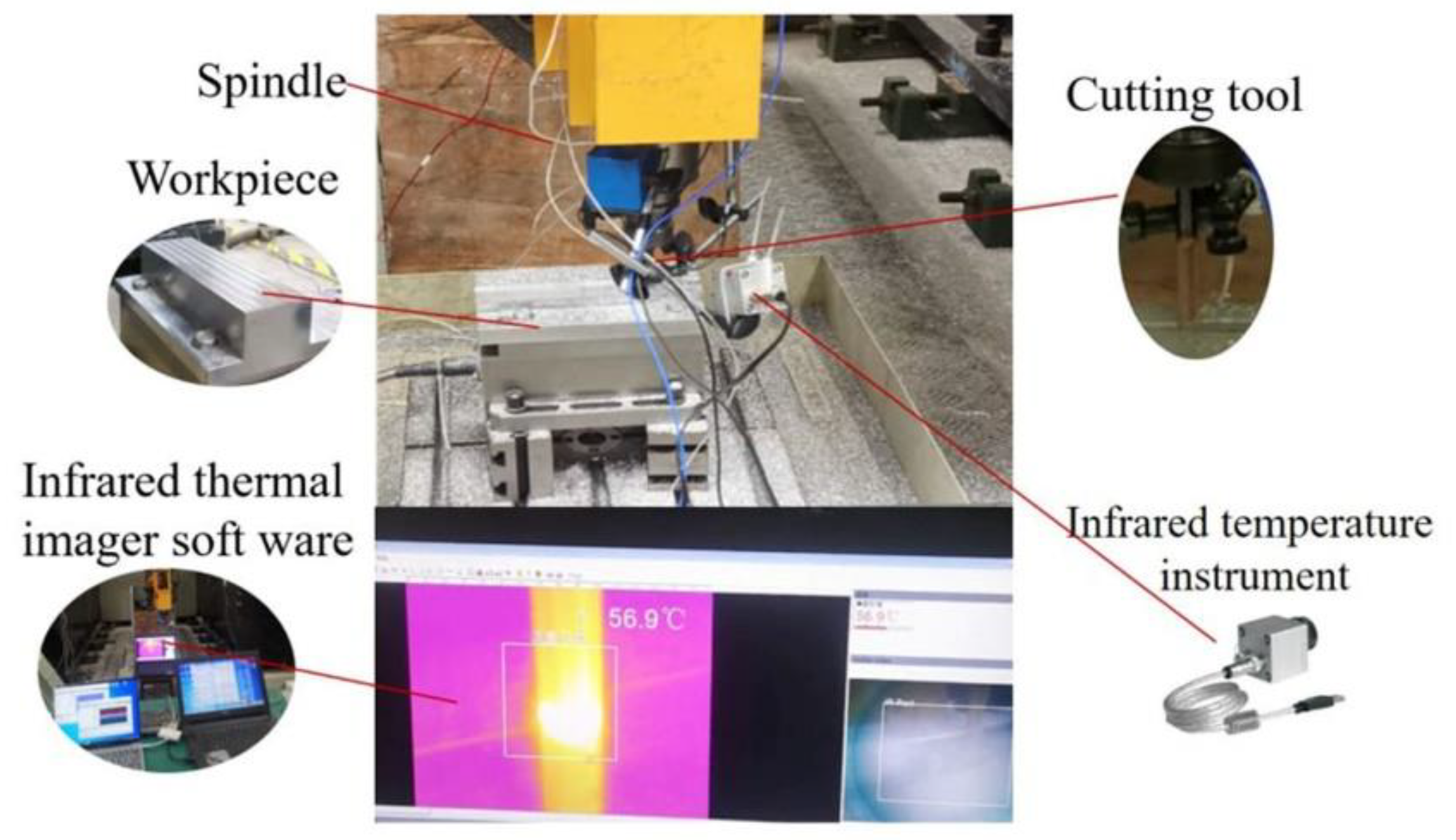
Figure 16.
Experimental setup to measure temperature rise based on equivalent tool deflection and friction.
Figure 16.
Experimental setup to measure temperature rise based on equivalent tool deflection and friction.
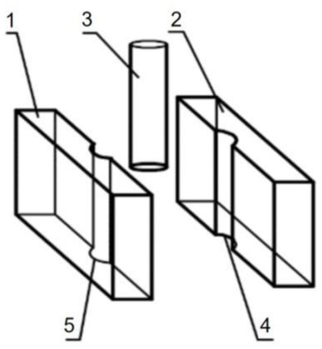
Figure 17.
Photograph of the setup for measuring the temperature rise due to tool deflection and friction.
Figure 17.
Photograph of the setup for measuring the temperature rise due to tool deflection and friction.

Figure 18.
3D temperature distribution of the X–Y direction section of the tool nose region.

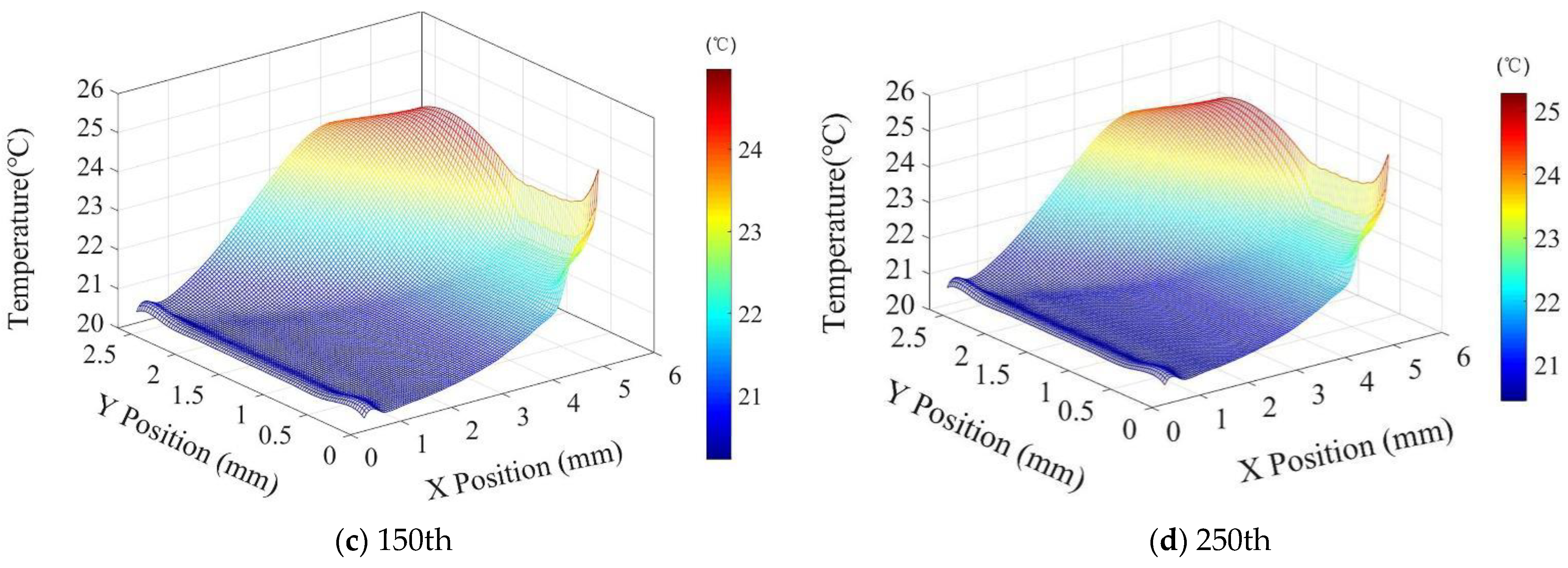
Figure 19.
Temperature gradient of the X–Y direction section of the tool nose region.
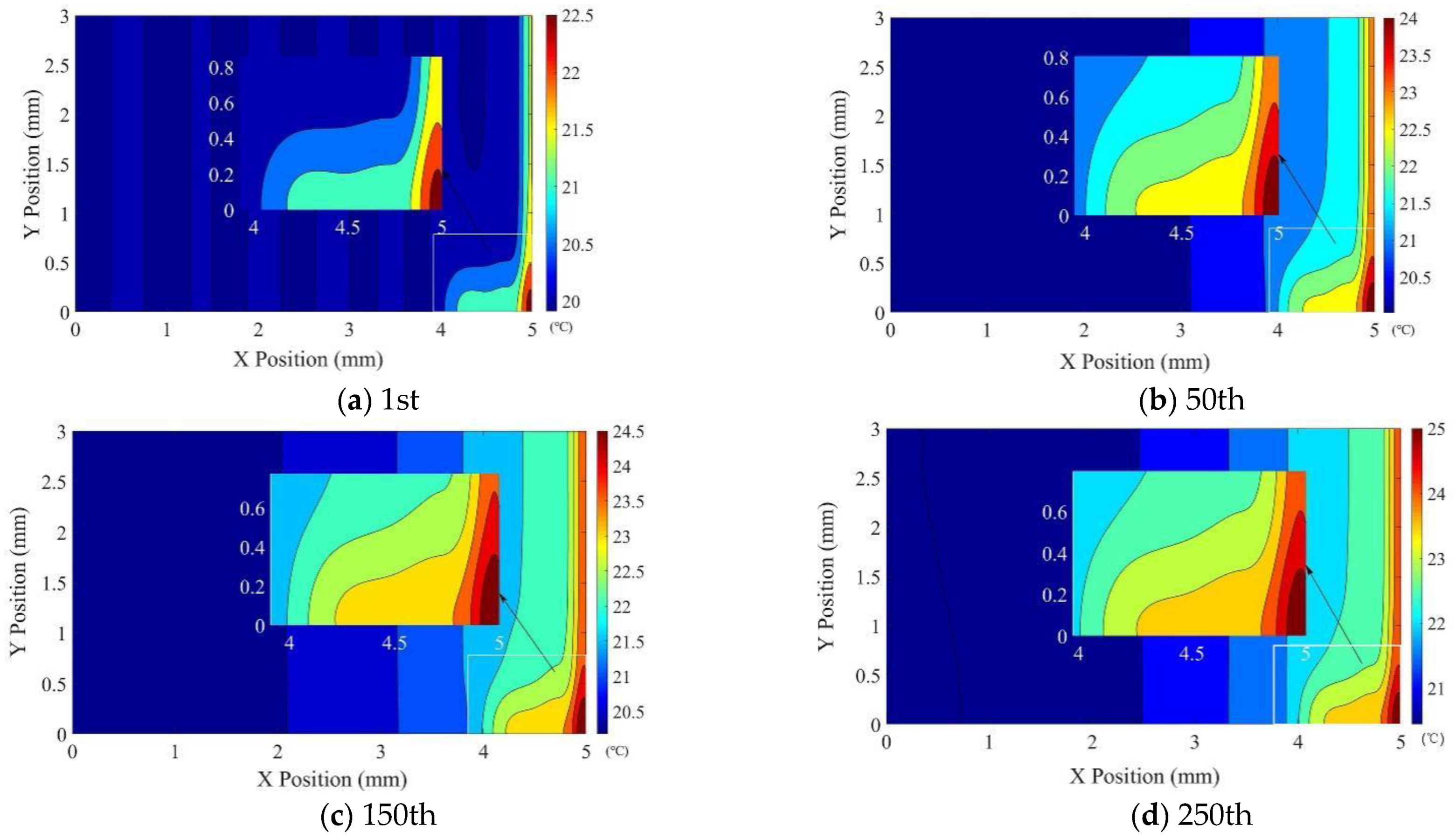
Figure 20.
Temperature measured in the experiments.


Table 1.
Geometric parameters and physical properties of the test tool.
| Parameter | Value |
|---|---|
| Diameter (mm) | 10 |
| Length (mm) | 70 |
| Blade length (mm) | 40 |
| Helix angle (°) | 35 |
| Number of teeth | 4 |
| Density (kg/cm3) | 14.8 |
| Young’s modulus (GPa) | 600 |
| Thermal conductivity (W/(m·K)) | 79.5 |
| Coefficient of thermal expansion (m/°C) | 5.2 |
| Specific heat (J/(kg·K)) | 209.2 |
Publisher’s Note: MDPI stays neutral with regard to jurisdictional claims in published maps and institutional affiliations. |
© 2021 by the authors. Licensee MDPI, Basel, Switzerland. This article is an open access article distributed under the terms and conditions of the Creative Commons Attribution (CC BY) license (https://creativecommons.org/licenses/by/4.0/).
Share and Cite
MDPI and ACS Style
Guo, Y.; Ye, W.; Xu, X. Numerical and Experimental Investigation of the Temperature Rise of Cutting Tools Caused by the Tool Deflection Energy. Machines 2021, 9, 122. https://doi.org/10.3390/machines9060122
AMA Style
Guo Y, Ye W, Xu X. Numerical and Experimental Investigation of the Temperature Rise of Cutting Tools Caused by the Tool Deflection Energy. Machines. 2021; 9(6):122. https://doi.org/10.3390/machines9060122
Chicago/Turabian StyleGuo, Yunxia, Wenhua Ye, and Xiang Xu. 2021. "Numerical and Experimental Investigation of the Temperature Rise of Cutting Tools Caused by the Tool Deflection Energy" Machines 9, no. 6: 122. https://doi.org/10.3390/machines9060122
Note that from the first issue of 2016, this journal uses article numbers instead of page numbers. See further details here.