
Optimal Design of Shift Point Strategy for DCT Based on Particle Swarm Optimization


Automotive Engineering Research Institute, Jiangsu University, Zhenjiang 212013, China
*
Author to whom correspondence should be addressed.
Machines 2021, 9(9), 196; https://doi.org/10.3390/machines9090196
Submission received: 28 July 2021
/
Revised: 3 September 2021
/
Accepted: 7 September 2021
/
Published: 10 September 2021
(This article belongs to the Section Vehicle Engineering)
Abstract
:For a vehicle equipped with DCT, the vehicle model is established according to the existing experimental data. The traditional method is used to solve the law of economic and dynamic shift, respectively. Then, the dynamic objective function and economic objective function are designed. After normalization of the two functions, the weighted combination is carried out to get the comprehensive objective function. The traditional shift law obtained in the previous paper is regarded as the limit value of variable optimization by particle swarm optimization algorithm, and the comprehensive objective function designed in this paper is solved. The shift law obtained by the three methods is integrated into Simulink model, and the dynamic and economic verification are carried out, respectively. By comparing the acceleration time of 0–100, 0–70, and 70–120 km/h, the dynamic performance of the shift point is obtained by three methods. The final test results show that the economy of the optimized shift point is improved by 1.37% and 3.17%, respectively. The power performance increased by 4.087%, 15.28%, and −10.70%, hence, achieving the desired results.
1. Introduction
Dual clutch transmission is becoming a hot research product in the category of automatic transmission [1,2,3,4]. In the optimization research of double clutch transmission [5,6], besides the coordination control of clutch [7,8,9], the formulation of shift law also deserves adequate attention [10,11,12,13,14,15,16]. Due to the different vehicle types [17,18], the transmission ratio and the matching power source are different [19]. In order to match the relationship between the transmission system and power system [20], this paper provides a method to optimize the shift point of transmission [21]. The transmission needs to be matched to the engine according to the characteristics of the engine, in order to improve its economy and power utilization. The specific fuel consumption is obtained by converting the original data when making the economic shift point and the fuel consumption rate is used as the reference of economical shift point. This method can ensure low fuel consumption under different driving cycles. A reasonable shift law can improve the vehicle’s power and economy, thus improving the vehicle’s comfort and driving experience. At present, domestic and international research scholars often use intelligent algorithm to study the shift law of multi-gear double clutch transmission and usually determine the shift point only according to a single performance index, which has low practical value and large promotion space. Wang Xu [1] put forward the concept of hybrid gear and designed the shift law by taking the optimum equivalent fuel consumption as the criterion. Although the result meets the economic requirements, the dynamic characteristics are not fully considered. Du Changqing et al. [6] put forward the optimization design method for DCT parameters of hybrid electric vehicle, considering the economy but not fully considering power. Liu Yonggang [4] separately formulated the traditional methods for the economic and dynamic shift rules of DCT, but did not optimize the combination. Luna et al. [11] made shift rules based on the combination of vehicle dynamics and economy. However, the validation model and performance evaluation index used by Luna are unreasonable, and the reliability is low. Guo et al. [21] proposed the shift control strategy of MPC. After verification, it was found that the economy of MPC increased by 4% on average under different operating conditions, without dynamic design and verification. Ruan et al. [18] have tested and verified the capability of DCT to reduce the cost and improve the efficiency of electric vehicles.
Considering that most of the working places for passenger cars are city roads and highways with relatively good road conditions, the actual speed has relatively large fluctuations, so on the basis of sufficient power, good economy should be pursued. In this paper, firstly, the power shift rule is made according to the power evaluation index, and then the economic shift rule is made according to the economy evaluation index. In order to obtain good economy, considering sufficient power, this paper establishes the target function of power evaluation index with the accelerated average change rate, and the target function of economy evaluation index with the average change rate of actual energy consumption. The total optimization objective function is obtained by weighting it. After obtaining the shift law by particle swarm optimization (PSO) based on the original traditional method [6,10], the modified shift law is obtained as the restriction of the optimization variable [22,23,24,25]. The simulation results show that the modified shift law can improve both economy and dynamics.
2. Topic
2.1. The Vehicle Layout
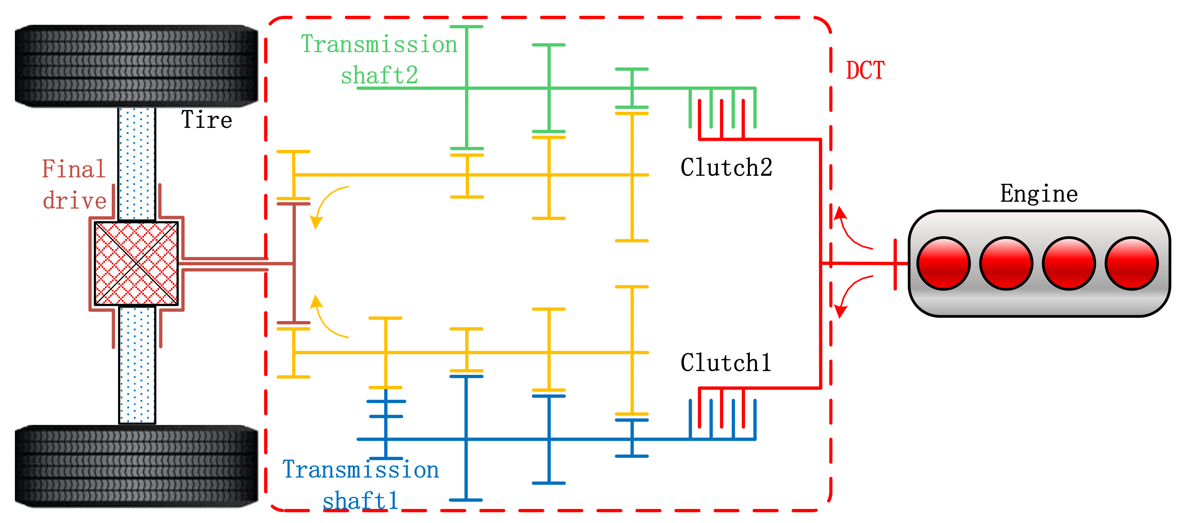
This paper studies the structure of the vehicle transmission equipped with a 6-gear DCT, as shown in Figure 1. The power of the engine is transferred to the final drive and finally to the driving wheel through the coordination between two clutches. As typical of double-clutch transmissions, there is no power interruption during shifting, and the driver will not feel a significant decrease in speed, which in turn can improve driving comfort by reducing longitudinal acceleration disturbances. On the basis of compact structure, improving the range of transmission speed ratio and smooth shifting can improve the overall transmission efficiency.
2.2. The Basic Parameters
Taking a test car as the research object, the shift rule of its Dual Clutch Transmission is formulated with comprehensive consideration of power and economy. The main vehicle parameters are shown in Table 1.
2.3. Operating Characteristics of Power System
3. Formulation of Shift Law
In the normal driving process of a car, the change of target gear caused by the change of shifting control parameters is called shifting law. According to the number of different control parameters, the shift law can be divided into single parameter shift law, double parameter shift law, and triple parameter shift law. The single-parameter shift law takes the speed as the reference quantity to implement the shift. Since the single-parameter shift law cannot reliably match the driver’s intention, the quality of the shift is poor. The triple-parameter shifting law takes the throttle opening throttle, vehicle speed v, and vehicle acceleration a as the input variables for shifting. Since the vehicle acceleration a is added into it, the up-slope and down-slope working conditions of the vehicle can be expressed. However, the formulation of its dynamic shifting law is complicated and difficult to implement. Throttle opening throttle and vehicle speed u are used as input variables for shifting of the two-parameter shifting law. Throttle opening throttle expresses the driver’s intention to a large extent, while vehicle speed u represents the current driving state of the vehicle. Compared with the three-parameter shift, the formulation and realization of the two-parameter shift rule is simple and easy to operate. Meanwhile, compared with the single-parameter shift, the driver’s intention is added, which is more in line with the concept of human-vehicle interaction. The equal delay shift strategy can ensure the stability of the shift process and reduce the shift cycle. The equal delay shift law can enter the high gear in advance when the throttle opening is low, so as to reduce the engine noise. The shift back to low gear can be delayed to improve fuel economy. When the throttle opening is large, the power can be maintained in a good state. Since the working condition considered in this paper is mainly flat road surface, and the working condition of up and down hill is not considered, the double parameter input is used in this paper to formulate the shifting law of vehicles.
3.1. Formulation of Power Shift Point Strategy
To ensure that the car has good power performance, enough reserve power for acceleration is the basic requirement of the power shift law. This situation can maximize the engine power utilization and vehicle traction characteristics [6]. In this paper, the basis for making the shift point is the acceleration (a) of the vehicle, and the vehicle speed (u) at the intersection of curves between adjacent gears is taken as the corresponding shift point at the same accelerator opening:
According to the above formula, the best dynamic shift point speed can be obtained in turn. After the vehicle speed at each shift point is obtained by fixing the throttle opening, the shift law of each gear can be formulated by delaying downshifting at the same speed. Finally, the mathematical model of shift law can be obtained by fitting.
The force analysis of a moving vehicle by means of vehicle system dynamics shows that the vehicle is driven by a certain driving force while in motion and is subject to certain acceleration resistance , air resistance , slope resistance , and rolling resistance [27].
This source data are a map of engine speed and torque, so by the following formula:
the relationship between the driving force and torque can be obtained. In the formula:
- is the transmission ratio;
- is the transmission ratio of final drive;
- is the mechanical transmission efficiency;
- is the wheel rolling radius (m).
The converted differential equation of vehicle motion is:
In the above formula:
- is the drag coefficient;
- A is the windward area of vehicles (m2);
- u is the vehicle speed (km/h);
- θ is the slope angle (°);
- δ is the rotating mass conversion factor;
- f is the coefficient of rolling resistance.
According to the formula:
The mathematical model of conversion coefficient of the rotating mass can be obtained:
- is the wheel moment of inertia (kg m2);
- is the moment of inertia of flywheel (kg m2).
After calculation, the conversion coefficient of rotation mass in the corresponding gear is obtained as follows:
Since the study does not consider the uphill and downhill conditions, the slope value is taken here.
Therefore, the above formula can be simplified as follows:
Additionally, we can get:
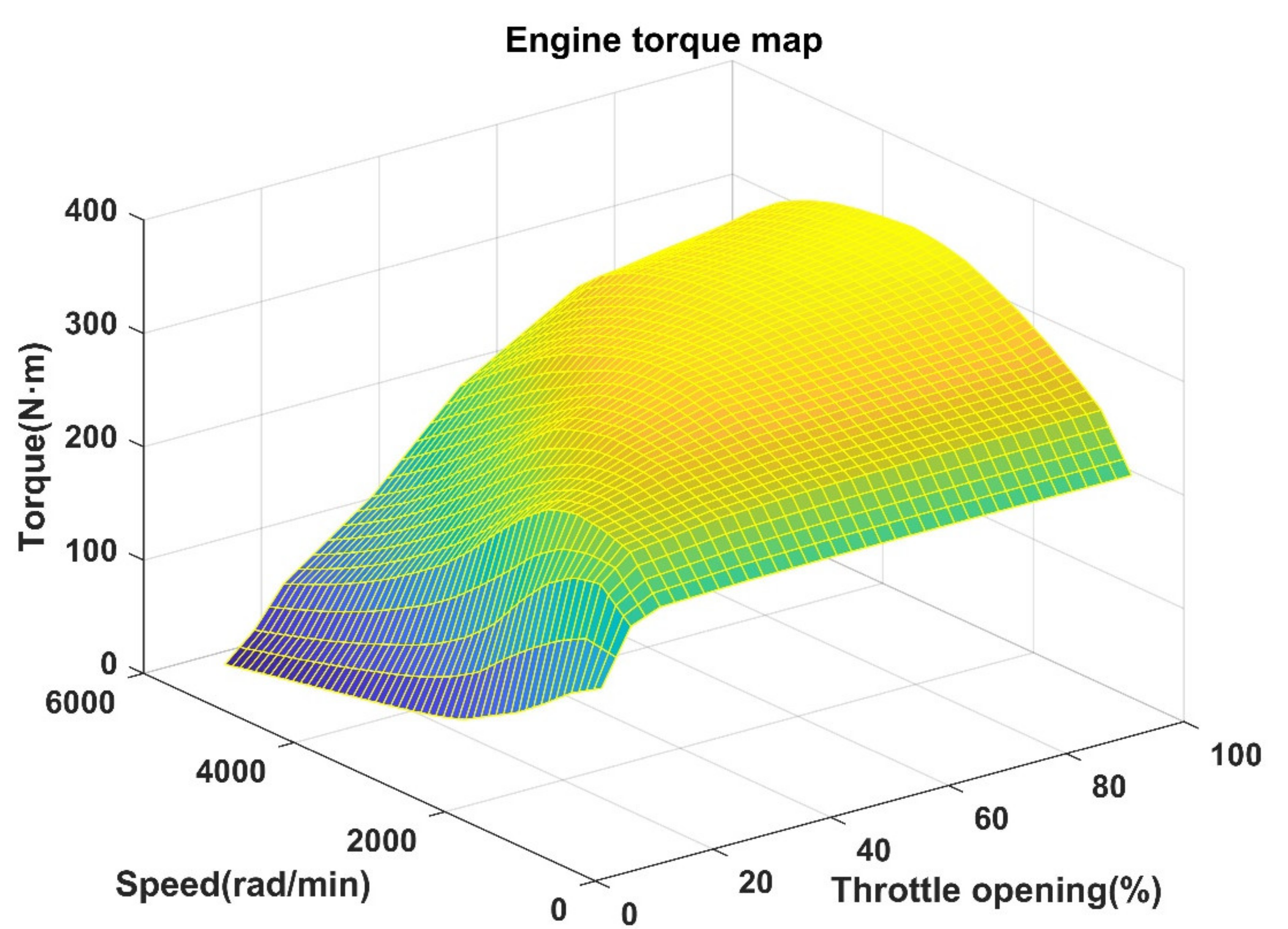
According to the engine calibration map, the calibration data between the torque and speed n is obtained by fixing the throttle opening α. In order to express the model accurately, the map data is accurately expressed with the mathematical formula by binary multiple polynomial fitting. The formula is as follows:
Here, , and etc. in the formula are constant coefficients obtained after fitting.
Where α is the throttle opening and n is the engine speed. The rest are constant parameters. relation can be obtained from the above formula. According to the above fitting formula, the torque fitting effect is shown in Figure 4:
Since has been obtained, the relation can be obtained.
The following equation can be obtained from relationship :
- is the nth gear ;
- is the (n + 1)th gear .
3.2. Establishment of Economical Shift Point
Based on the specific fuel consumption , the mathematical relationship between the engine output torque and is found by fixing the throttle opening in the relationship between the specific fuel consumption and vehicle speed.
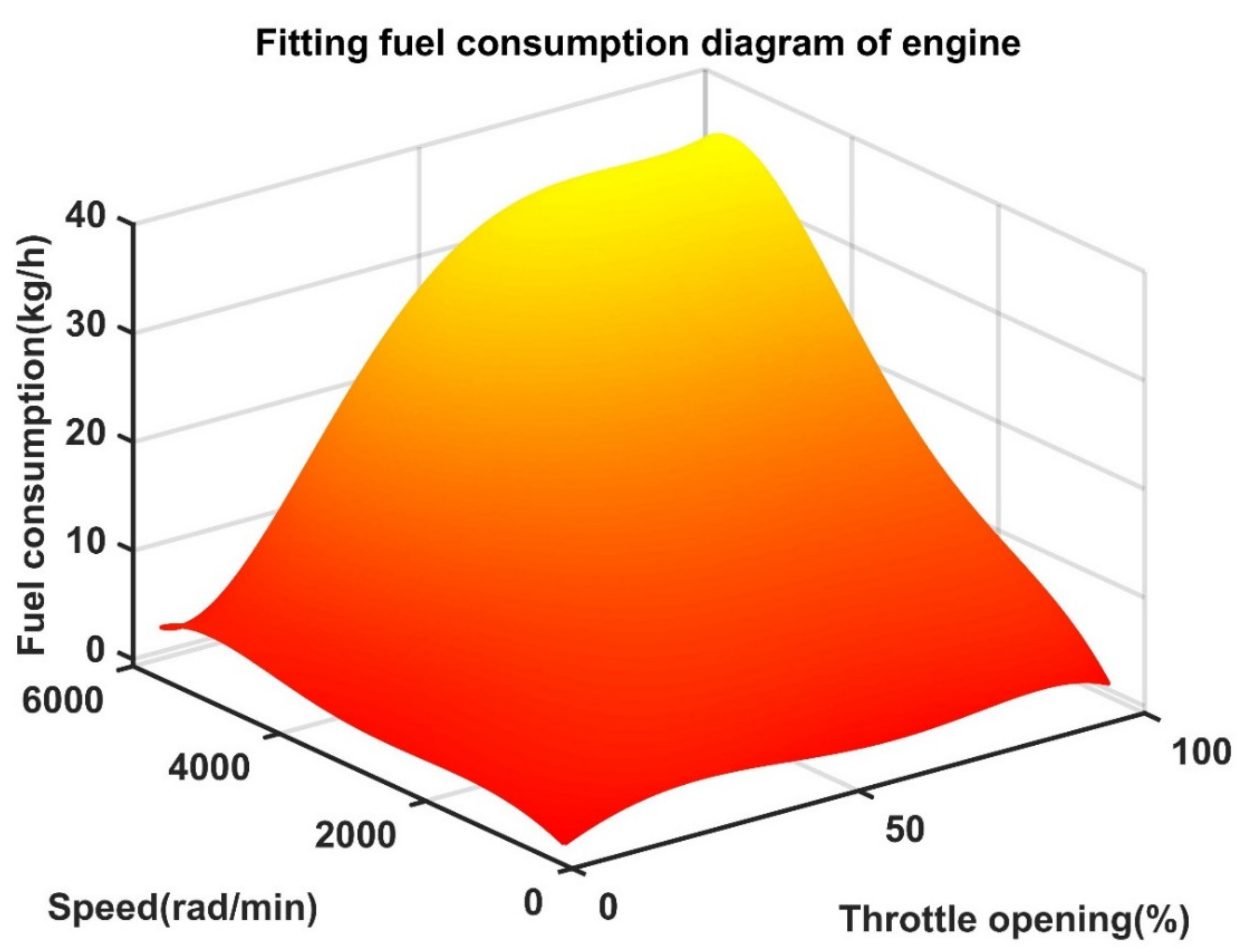
More accurate and detailed data can be obtained by bilinear interpolation of the original fuel consumption data from the engine bench test. In order to further optimize and obtain the accurate fuel consumption model, the processed data are fitted by binary multiple polynomial, and the expression is as follows:
In this formula, , etc. are constant coefficients obtained after fitting. According to the above fitting formula, the fitting effect of engine fuel consumption is shown in Figure 6:
- b is the specific fuel consumption (g/(kW·h));
- is the fuel consumption (mL/s);
- is the engine power (kW·h);
- ρ is the fuel density (kg/L);
- g is the gravity acceleration (m/s2).
In this formula:
After conversion, the simplified fuel consumption rate formula can be obtained as follows:
In this formula:
is the fuel consumption (L/h).
According to the engine fuel consumption curve, the experimental data between the engine fuel consumption and torque speed can be obtained. Bilinear interpolation can be used to expand the data. In order to get an accurate mathematical model, the modified data are used to fit the three-dimensional surface. The final formula is the bivariate multiple polynomial function:
The specific expression is as follows:
The function relationship between the fuel consumption ratio, speed and throttle opening can be obtained by combining the engine torque characteristic curve:
Since the function between the engine output speed and vehicle speed is as follows:
A functional relationship between the fuel consumption ratio, vehicle speed and throttle opening can therefore be obtained:
Through the above conversion, we can get the formulation formula of the economic shift point based on the fuel consumption ratio as the evaluation index:
The above formula and data are programmed by MATLAB. As the throttle opening in the formula is also a parameter in the formula, the shift point results under different throttle opening can be obtained by the programming assignment and then running. Due to the accurate fitting results, it is convenient to calculate the shift point and simplify the operation. Since the original data fluctuates greatly when the throttle opening is less than 20%, thus 20% of the throttle opening is taken as the initial shift throttle opening. The upshift strategy of Figure 7 is obtained by interpolation, and the specific data are shown in Table 3.
3.3. Shift Point Establishment Based on Particle Swarm Optimization
Particle swarm optimization (PSO) was first proposed by American scholars Kennedy and Eberhart in 1995. Its basic idea is inspired by the research results of modeling and Simulation of bird group behavior.
The core of particle swarm optimization algorithm is to simulate the behavior of birds. The individuals in the birds share the information, which promotes the evolution of subsequent solutions using the intermediate information. It makes the movement behavior of the whole group have an evolution process from disorder to order in the problem solving space, which greatly improves the search efficiency and makes it easier to find an accurate feasible solution. The above logic is shown in Figure 8.
In this paper, when the optimization algorithm is preliminarily selected, other intelligent algorithms such as particle swarm optimization algorithm, dynamic programming method, and extreme value principle were preselected. Compared with other intelligent algorithms, the PSO algorithm has no crossover and mutation operation, and relies on the speed between adjacent particles to complete its search. In the process of iterative evolution, only the optimal particle can transfer information to other particles, and at fast search speed. The PSO algorithm has memory, and the optimal position in each iteration process can remember and transfer the position information to other particles. The PSO algorithm needs less parameters. The utility model has the advantages of simple structure and easy engineering realization. The algorithm has fast convergence speed and low hardware requirements. Among them, the particle swarm optimization algorithm has some disadvantages, such as lack of dynamic adjustment of speed and ease to fall into local optimization. The solution of this problem is to solve it many times and take the optimal solution. Other disadvantages include the need to limit the range of parameters and the need to consider practical problems for parameter control. This problem can be solved by taking the power and economic shift law solved above as the limit of its optimization range. Based on the above advantages and disadvantages, this paper selects PSO as the optimization algorithm. Since the main innovation of this paper lies in the formulation of the optimization objective function integrating economy and power, there is no optimization innovation at the algorithm level. This paper focuses on the practicability and operability of the algorithm. As a classical algorithm, PSO has been widely used and verified by a large number of scholars [9,25]. Therefore, owing to space limitation, this paper does not compare this algorithm with other algorithms. However, the introduction of this algorithm greatly improves the solution speed of the objective function. The flow chart of PSO specific optimization algorithm in this paper is shown in Figure 9 [28].
In this paper, the total objective function is composed of dynamic objective function and economic objective function. The particle is the candidate solution of the optimization problem; position is the position of the candidate solution; speed is the speed of the candidate solution; fitness is the value of evaluating the solution, which is generally set as the objective function value; the best position of individual is the best position found by a single particle so far; and the best position of group is the best position found by all the particles so far.
3.3.1. The Establishment of Objective Function
The dynamic evaluation index is the average change rate of acceleration:
The two objective functions need to be de dimensionalized. Here, the objective function after adopting the normalized de dimensioning method is as follows:
In this formula,
- n is the n gear;
- is the n gear acceleration (m/s2);
- is the gear acceleration (m/s2).
The acceleration formula is , and the significance of each parameter has been given.
Generally, the specific fuel consumption is used as the economic evaluation index, or the actual energy consumption of the whole vehicle, that is, the integral of output power to time, is used as the evaluation index. In this paper, the average change rate of the energy consumption of the whole vehicle power system is taken as the economic evaluation index. The total energy consumption includes the sum of the accumulated fuel consumption of the vehicle working in gears 1 to 6. The calculation method is to obtain the equivalent energy consumption by integrating the specific fuel consumption with time. After de dimensioning and normalization, the economic evaluation index can be expressed as follows:
In the above formula .
The dynamic and economic objective functions are combined and weights and are added. The total objective function is:
where:
- is the weighting coefficient of dynamic index;
- is the weighting coefficient of economic indicators.
3.3.2. Determination of Optimization Variables
Since all the relevant parameters of the DCT system have been determined, the main parameters affecting its dynamics and economy are accelerator pedal opening α and vehicle speed v at shift point. Since the design weight in this paper is a dynamic parameter, and are variables and . Therefore, it is sufficient to determine the weight variable in this paper only to optimize . The total optimization variables are:
Among them, indicate the speed at shift point of i gear at throttle openings of 15%, 20%, and 100%, respectively.
Variable Constraints
In order to reduce the particle swarm optimization time, improve the optimization efficiency, and optimize the results, the large speed difference of the shift points in different gears is considered. At the same time, as the economic shift point tends to shift earlier, the dynamic shift point tends to shift later. Therefore, economic shift points at different throttle openings are considered as and dynamic shift points as . Therefore, the particle optimization range is shortened and the -optimization interval is limited.
3.3.3. Particle Swarm Optimization Solution Application
In combination with the number of optimization variables in the objective function, the number of particles in the particle swarm is set to 100. Since the inertia weight of MATLAB can be adapted, the inertia weight can adopt the adaptive neighborhood mode at the beginning of searching for the optimal solution, which is convenient to divide the particles into groups and groups of different groups at the beginning, search for multiple groups of local optimum in different regions, and find the local optimum solution as soon as possible to reduce the iteration time. When fitness begins to stagnate, its particle swarm search mode begins to shift to the global mode and fitness begins to decline, then it returns to the neighborhood mode to avoid falling into local optimum. The fitness stagnates several times until the number of stagnation times is greater than the judgement value, and the inertia coefficient decreases gradually, which is conducive to the centralized particles seeking the fitness in the optimal domain. Therefore, only the given inertia weight range is required for this method as [0.1, 1.1].
The method of reference compression factor for individual learning factors and social learning factors is set as 1.49.
The proportion of particles in the neighborhood is 0.25.
The above comprehensive objective function and setting parameters are programmed with MATLAB, and the final upshift and shift points of each gear are obtained as shown in Figure 10.
4. Simulation Results and Analysis
4.1. Establishment of Simulation Verification Model
A complete vehicle model with dual clutch transmission is built through Simulink. The model power system data use the engine data mentioned above. The model is divided into the driver model, power system, drive system and other modules. The new European driving cycle (NEDC) and worldwide light-duty test procedure (WTLC) operating conditions are taken as model inputs and the corresponding accelerator pedal opening and brake pedal opening are output through the driver model. The driver model is shown in Figure 11. Acceleration and braking of the entire vehicle is thus achieved. Economic shift strategy, dynamic shift strategy, and integrated optimization shift strategy are put into the simulation model to run, and are compared. By observing the dynamic and economic evaluation indexes after the simulation operation, the comparison of dynamic and economic before and after optimization is achieved. The vehicle control strategy model is shown in Figure 12.
4.2. Analysis of Economic Validation Results
When verifying the energy consumption on the built simulation platform, the adaptability and stability of the optimization results can be investigated using different driving cycles. In this paper, the more traditional and classic NEDC and WLTC working conditions are selected for verification. Figure 13 shows the NEDC and WLTC working conditions. The NEDC working condition on the left in Figure 13 has a total duration of 1180 s and a maximum speed of 120 km/h. It has frequent start and stop common in urban cycle, which can represent the classic urban working condition. In Figure 13, the total duration of WLTC working condition on the right side is 1800 s and the maximum speed is 131.3 km/h. It also has the frequent start and stop working condition of urban cycle. Moreover, compared with NEDC, the acceleration in WLTC working condition is usually nonlinear. Therefore, WLTC is closer to the actual situation. Unifying the two driving cycles for analysis is conducive to verify the reliability of shift law and the robustness of optimization algorithm.
The economic shift point, dynamic shift point, and synthetically optimized shift point are input into the vehicle simulation platform for the NEDC and WTLC operating condition test. The simulation results are shown in Figure 14.
Figure 14 shows that the speed following condition yields a good result, the difference between the simulated actual speeds corresponding to the three different shift points is small, there is no obvious fluctuation, and the overall speed following condition is good, which can ideally achieve the acceleration and deceleration within the specified time. However, there will be a slight jitter in the dynamic shift strategy when the speed is lowered. This also indicates that the economic shift strategy has better shift quality than the dynamic shift strategy for the same vehicle with different shift strategies. This slight jitter in speed during shifting is due to the power interruption of the vehicle during shifting. This situation can be optimized by taking into account the motion control of the two clutches in a dual clutch transmission in order to reduce speed fluctuations. The speed shown in Figure 15 is in good condition, and the actual vehicle speed corresponding to the three different shift rules is basically the same. Therefore, the fuel consumption results before and after optimization are of comparative significance, and the fuel consumption error caused by the driver model can be ignored.
Figure 16 shows the change of three gears under different shift strategies under NEDC and WLTC operating conditions. It can be seen from the NEDC operating condition that the most frequent shift is the optimized shift strategy, while the lower shift number is the dynamic shift strategy since it spends more time driving in low gear. The reason is that the first 800 s are complicated and the congestion conditions and the vehicle speed are low. The optimized shift point speed is higher than the economic shift point speed and lower than the power shift point speed. Therefore, the simulation results of the optimized shift strategy show that it shifts frequently. However, due to the low speed in the first 800 s, only four gears appear in the simulation results of dynamic shift strategy. However, there are no frequent shifting, random shifting, and other conditions in this paper, which show that the delay shift strategy used in this paper is reasonable. Comparing the energy consumption diagram of the model operation under this condition, we can get a NEDC condition, under which the energy consumption of the optimized shift strategy is reduced by 1.37% and 23.00%, respectively compared with the economical and dynamic shift strategy. It can be seen from Figure 17 that the energy consumption is reduced and the emission is improved after the model shift law is optimized. This is mainly due to the reduced low gear operating conditions and the increased running time of the vehicle in the engine efficiency range. Similarly, the gears change frequently in the WLTC working condition, since the target vehicle speed changes frequently with time. Compared with the energy consumption in Figure 17 of model operation under the WLTC condition, it can be obtained that under the WLTC condition, the energy consumption of the optimized shift strategy is reduced by 3.18% and 13.18%, respectively compared with the economic and dynamic shift strategy. The data analysis results are shown in Table 4.
By analyzing the two driving cycles, it can be obtained that the optimized shift law has obvious advantages. From the above simulation results, the shift law obtained from the optimization results can obtain better fuel economy under the condition of ensuring power following.
4.3. Analysis of Dynamic Verification Results
The input working condition is changed to verify the vehicle dynamic performance, in order to improve the reliability of the dynamic verification results in this paper. Here, two driving cycles are used to verify the dynamic performance, and three evaluation indexes are used to comprehensively evaluate the dynamic performance.
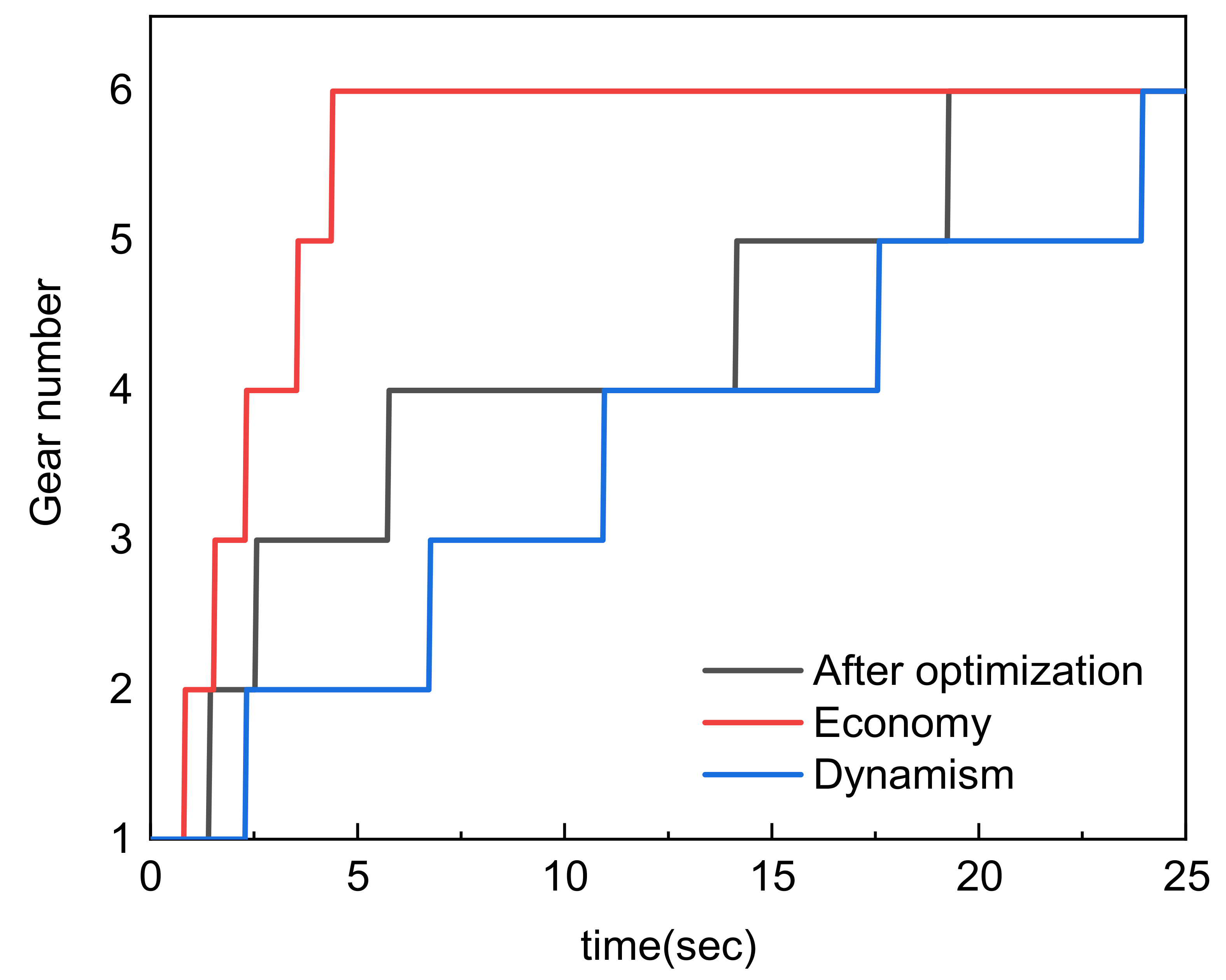
The first dynamic performance verification condition is the initial throttle opening is 0%, which rises to 100% at a constant speed within 1 s and remains unchanged. The specific working conditions are shown in Figure 18. The dynamic evaluation index here adopts the acceleration time of 100 km. Through the simulation results, it can be concluded that the comprehensive shift law accelerates to 100 km/h after 14.08 s, the vehicle with economic shift law needs 24.4 s to accelerate to 100 km/h under the same driving cycles, and the vehicle with dynamic shift law needs 14.68 s to accelerate to 100 km/h. The schematic diagram of simulation shift results under this working condition is shown in Figure 19. Compared with the simulation results, it can be obtained that the power performance index of the vehicle with optimized shift law is increased by 4.087% compared with the vehicle with dynamic shift law. The power performance of the vehicle with optimized shift law is 42.30% higher than that with economic shift law. The simulation results are shown in Figure 20. The data analysis results are shown in Table 5.
The second dynamic performance verification condition is consistent with the first dynamic performance verification condition. The evaluation index adopts the acceleration time of 0–70 km/h. The simulation results show that the acceleration time of vehicles with comprehensive shift law is 7.21 s, the acceleration time of vehicles with economic shift law is 12.89 s, and the acceleration time of vehicles with dynamic shift law is 8.51 s. The comparative simulation results show that the power performance of the vehicle with optimized shift law is 15.28% higher than that with dynamic shift law. Compared with the vehicle with economic shift law, the power performance of the vehicle with optimized shift law is improved by 44.07%. It shows that in the front acceleration process of the vehicle, the vehicle acceleration power using the optimized shift law is very strong. The simulation results are shown in Figure 21. The data analysis results are shown in Table 6.
The third dynamic performance verification condition is: Use the driver model to control the initial speed of the vehicle at 70 km/h, and then adjust the accelerator pedal opening to 100% within 0.5 s. The dynamic evaluation index here adopts the acceleration time of 70–120 km/h. The simulation results show that the acceleration time of vehicles with comprehensive shift law is 15.33 s, the acceleration time of vehicles with economic shift law is 20.58 s, and the acceleration time of vehicles with dynamic shift law is 13.69 s. Compared with the simulation results, it is found that the dynamic index of the vehicle with optimized shift law is reduced by 10.70%. Compared with the vehicle with economic shift law, the power performance of the vehicle with optimized shift law is improved by 25.51%. It shows that there are some deficiencies in the vehicle acceleration power using the optimized shift law in the process of vehicle rear section acceleration. The simulation results are shown in Figure 22. The data analysis results are shown in Table 7.
Based on the above three comparison results, it can be obtained that the power performance of the optimized shift point is significantly improved. Especially in the acceleration process of the first half of the vehicle starting, the power is sufficient. At 70–120 km/h, although the power decreases, the overall power is strong. Therefore, the optimization results are good.
5. Conclusions
In this paper, a vehicle with six speed dual clutch transmission is introduced. Firstly, the engine bench test is carried out to get the map of engine fuel consumption and engine torque. Based on the inherent parameters of the vehicle and the engine performance data obtained from the bench test, the two-parameter shift law is formulated using traditional methods based on fuel economy and dynamics, respectively. According to the simplified parameters of the vehicle, the shift law model is established, and the dynamic objective function and economic objective function are normalized and weighted to get the comprehensive optimization objective function. The comprehensive shift law is formulated by particle swarm optimization. According to the shift law obtained by traditional methods, it is taken as the reference limit of the range of variables to be optimized to reduce the particle swarm optimization time and enhance the particle swarm optimization effect. Finally, the dynamic diagram of adaptability varying with optimization times is obtained by programming in MATLAB, and the optimized shift law is obtained. By substituting the optimized shift law and the shift law before optimization into the power and economy evaluation indexes, the simulation results show that when the acceleration time of 0–100 km/h is used as the evaluation index, the improvement rate of dynamic performance can reach 4.087%. Taking the acceleration time of 0–70 km/h as the evaluation index, the improvement rate of dynamic performance can reach 15.28%. Taking the acceleration time of 70–120 km/h as the evaluation index, the improvement rate of power performance is −10.70%, that is, the power decreases. This also shows that the overall dynamic performance of the optimization results is good, the first half of the power is sufficient, but the second half of the power is poor. This is also the inevitable loss caused by the improving economy. The simulation results show that the improvement rate of fuel economy can reach 1.37% under the NEDC condition. The simulation results show that the economic improvement rate can reach 3.18% under the WLTC condition. By synthesizing the simulation results of the two driving cycles, it is found that the optimized shift law has good adaptability and stability.
The comprehensive optimization objective function developed in this paper combines the dynamic target with the economic target after normalizing, and determines the dynamic relationship between acceleration and specific fuel consumption. After checking the mathematical model, it is found that the final shift law can comprehensively improve the power and economy of the entire vehicle, taking both into account. The shift law obtained by this research method will be finally applied to the actual vehicle to verify, and the result is of great significance to the matching of power system and transmission system and the improvement of vehicle performance. This method provides an important reference value for optimization calculation of shift points of other transmission systems.
Author Contributions
Conceptualization, X.Y., X.S. and H.Z.; methodology, X.Y.; software, X.Y., J.L. and H.Z.; validation, X.Y. and J.L.; formal analysis, X.Y. and J.L.; investigation, X.Y.; resources, H.Z.; data curation, X.S.; writing—original draft preparation, X.Y.; writing—review and editing, X.Y.; visualization, X.Y.; supervision, X.Y.; project administration, X.S. and H.Z.; funding acquisition, X.S. and H.Z. All authors have read and agreed to the published version of the manuscript.
Funding
This research was funded by The Initial funding for Advanced Talents at Jiangsu University, grant number 13JDG034 and The APC was funded by Jiangsu University.
Institutional Review Board Statement
Not applicable.
Informed Consent Statement
Not applicable.
Data Availability Statement
Not applicable.
Acknowledgments
This work was supported by the Primary Research and Development Plan of Jiangsu Province under grant BE2017129 and The Initial funding for Advanced Talents at Jiangsu University under grant 13JDG034.
Conflicts of Interest
The authors declare no conflict of interest.
References
- Wang, X.; Huang, Y.; Yue, Y.; Li, G. Research on DCT Economic Shift Law of Parallel Hybrid Electric Vehicle. J. Automot. Eng. 2020, 10, 250–262. [Google Scholar]
- Tu, B. Research on Automatic Transmission Control of New 7-Speed Opposed Double Clutch Transmission. Master’s Thesis, Hefei University of Technology, Hefei, China, 2017. [Google Scholar]
- He, N.; Zhao, Z.; Li, Y. Shift regularity and simulation evaluation of double clutch automatic transmission. China Mech. Eng. 2011, 22, 367–373. [Google Scholar]
- Liu, Y. Research on Comprehensive Matching Control of Dual Clutch Automatic Transmission System of Passenger Car. Master’s Thesis, Chongqing University, Chongqing, China, 2010. [Google Scholar]
- Li, J. Shift law analysis and Simulation of double clutch transmission. Master’s Thesis, Hefei University of Technology, Hefei, China, 2012. [Google Scholar]
- Du, C.; Cao, X.; He, B.; Ren, W. Optimum design of parameters of dual clutch transmission based on hybrid particle swarm optimization. J. Jilin Univ. 2020, 50, 1556–1564. [Google Scholar]
- Deng, H. Research on Non-Powered Interrupt Shift Control Strategy for AMT Parallel Hybrid Electric Vehicle. Master’s Thesis, Jiangsu University, Zhenjiang, China, 2019. [Google Scholar]
- Yu, J.; Wu, C.; Hu, Y.; Mou, J. Characteristic analysis of new hybrid hydro mechanical composite transmission. J. Jiangsu Univ. Nat. Sci. Ed. 2016, 37, 507–511. [Google Scholar]
- Zhou, S.; Walker, P.; Wu, J.; Zhang, N. Power on gear shift control strategy design for a parallel hydraulic hybrid vehicle. Mech. Syst. Signal Process. 2021, 159, 107798. [Google Scholar]
- Tang, P.; Mao, Z.; Cai, Z. Research on Economic Shift Rule of Electric Vehicle Using Immune Particle Swarm Optimization. J. Chongqing Univ. Technol. 2021, 35, 67–74, 144. [Google Scholar]
- Luna, G.L.; Qu, J.; Guo, Z.; Mi, J.; Zhao, Z. Research on Comprehensive Shift Rule of TBW Automotive Based on Particle Swarm Optimization. J. Guangxi Univ. 2019, 44, 647–656. [Google Scholar]
- Liu, D. Research on Shift Rule of Full-Electricity AMT. Master’s Thesis, Central South University of Forestry Science and Technology, Changsha, China, 2015. [Google Scholar]
- Zhan, C.; Wang, Q.; Zhu, D.; Sui, H. AMT Shift Rule Design of Hybrid Electric Vehicle Based on Intelligent Optimization. Eng. 2020, 36, 110–116. [Google Scholar]
- Hou, R.; Zhang, J.; Lin, C. New Approach of Comprehensive Shift Schedule Based on Electric Drive Automated Mechanical Transmission. Energy Procedia 2016, 88, 945–949. [Google Scholar]
- Li, H.; He, H.; Peng, J.; Li, Z. Three-parameter Shift Schedule of Automatic Mechanical Transmission for Electric Bus. Energy Procedia 2018, 145, 504–509. [Google Scholar]
- Wang, J.; Liu, Y.; Liu, Q.; Xu, X. Power-based Shift Schedule for Pure Electric Vehicle with a Two-speed Automatic Transmission. IOP Conf. Ser. Mater. Sci. Eng. 2016, 157, 012016. [Google Scholar]
- Tian, F. 8AT Automatic Transmission Transmission Ratio Calculation and Shift Law Research and Simulation. Master’s Thesis, Northeast Forestry University, Harbin, China, 2020. [Google Scholar]
- Ruan, J.; Walker, P.; Zhang, N. A comparative study energy consumption and costs of battery electric vehicle transmissions. Appl. Energy 2016, 165, 119–134. [Google Scholar]
- Nguyen, C.T.; Walker, P.D.; Zhang, N. Shifting strategy and energy management of a two-motor drive powertrain for extended-range electric buses. Mech. Mach. Theory 2020, 153, 103966. [Google Scholar]
- Lin, C.; Zhao, M.; Pan, H.; Yi, J. Blending gear shift strategy design and comparison study for a battery electric city bus with AMT. Energy 2019, 185, 1–14. [Google Scholar]
- Guo, L.; Li, G.; Gao, B.; Chen, H. Shift Schedule Optimization of 2-Speed Electric Vehicle Using Model Predictive Control. In Proceedings of the 33rd Chinese Control Conference, Nanjing, China, 28–30 July 2014; IEEE: Piscataway, NJ, USA, 2014; Volume 6. [Google Scholar]
- Kennedy, J.; Eberhart, R. Particle swarm optimization. In Proceedings of the ICNN’95 International Conference on Neural Networks, Perth, WA, Australia, 27 November–1 December 1995; IEEE: Piscataway, NJ, USA, 1995. [Google Scholar]
- Sun, W.; Zhang, G.; Liu, L.; Qin, Y.; Zhang, X. Thermal parameter inversion of hydration heat process of concrete box girder based on standard particle swarm optimization algorithm. J. Jiangsu Univ. Nat. Sci. Ed. 2019, 40, 608–613, 620. [Google Scholar]
- Ren, W.; Hao, Z.; Wang, Y.; Xu, J. Application of improved particle swarm optimization algorithm in 3D hydrofoil design. J. Jiangsu Univ. Nat. Sci. Ed. 2017, 38, 168–172. [Google Scholar]
- Wu, X. Research and Application of Multi-objective Particle Swarm Optimization. Master’s Thesis, Nanjing University of Posts and Telecommunications, Nanjing, China, 2016. [Google Scholar]
- Fu, X.; Tie, X.; Liu, H. Energy management of hybrid off-road vehicle based on power demand prediction. J. Jiangsu Univ. Nat. Sci. Ed. 2021, 42, 67–76. [Google Scholar]
- Yu, Z. Automotive Theory; Machine Industry Press: Beijing, China.
- Zhao, S.; Zheng, Q.; Liu, H. Power system matching and Simulation of hybrid logistics vehicle. J. Jiangsu Univ. Nat. Sci. Ed. 2020, 41, 648–654. [Google Scholar]
Figure 1.
Transmission diagram of dual clutch transmission.

Figure 2.
Engine torque map.

Figure 3.
Engine fuel consumption map.

Figure 4.
Fitting torque diagram of engine.
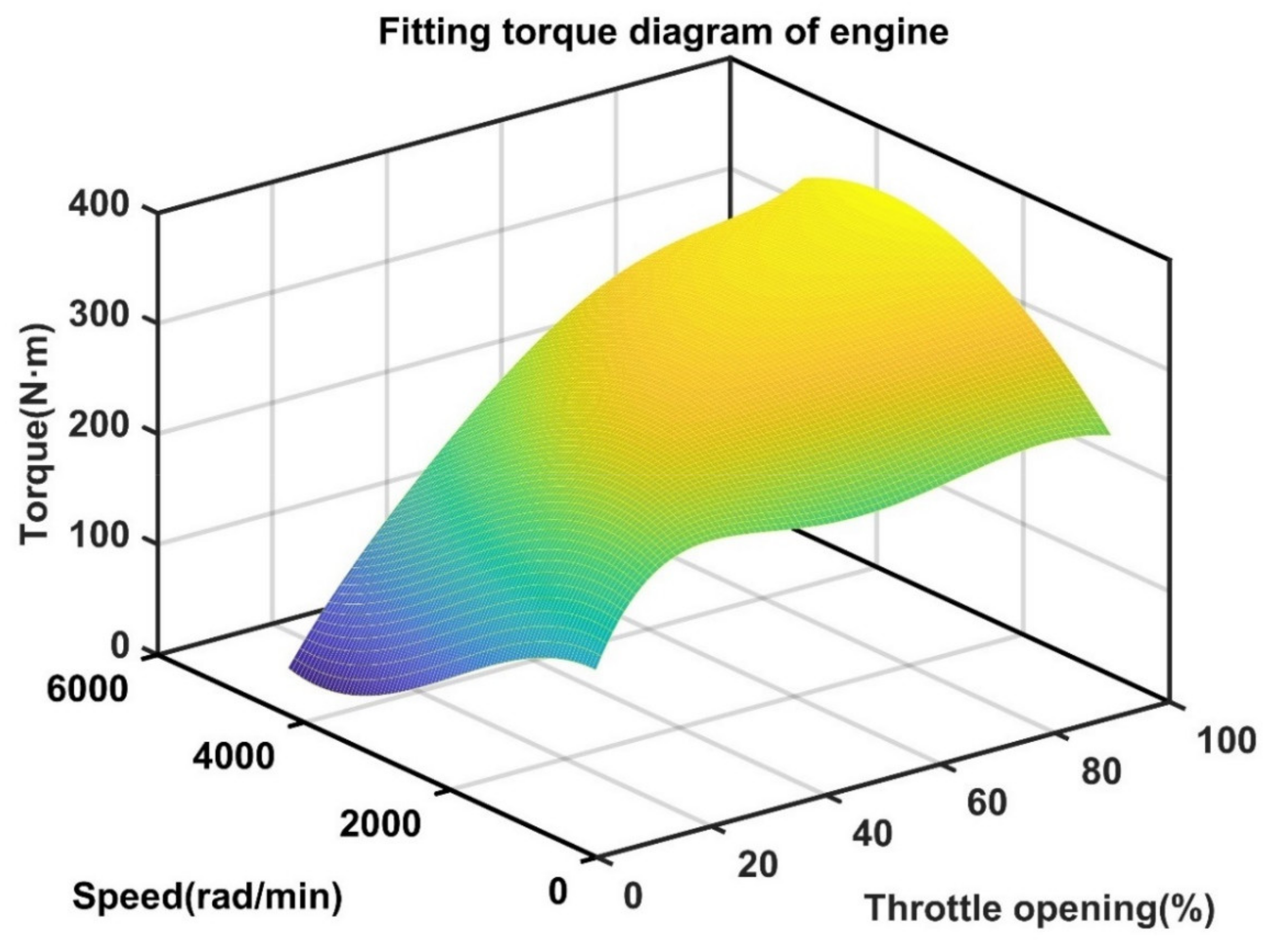
Figure 5.
Dynamic upshift point.
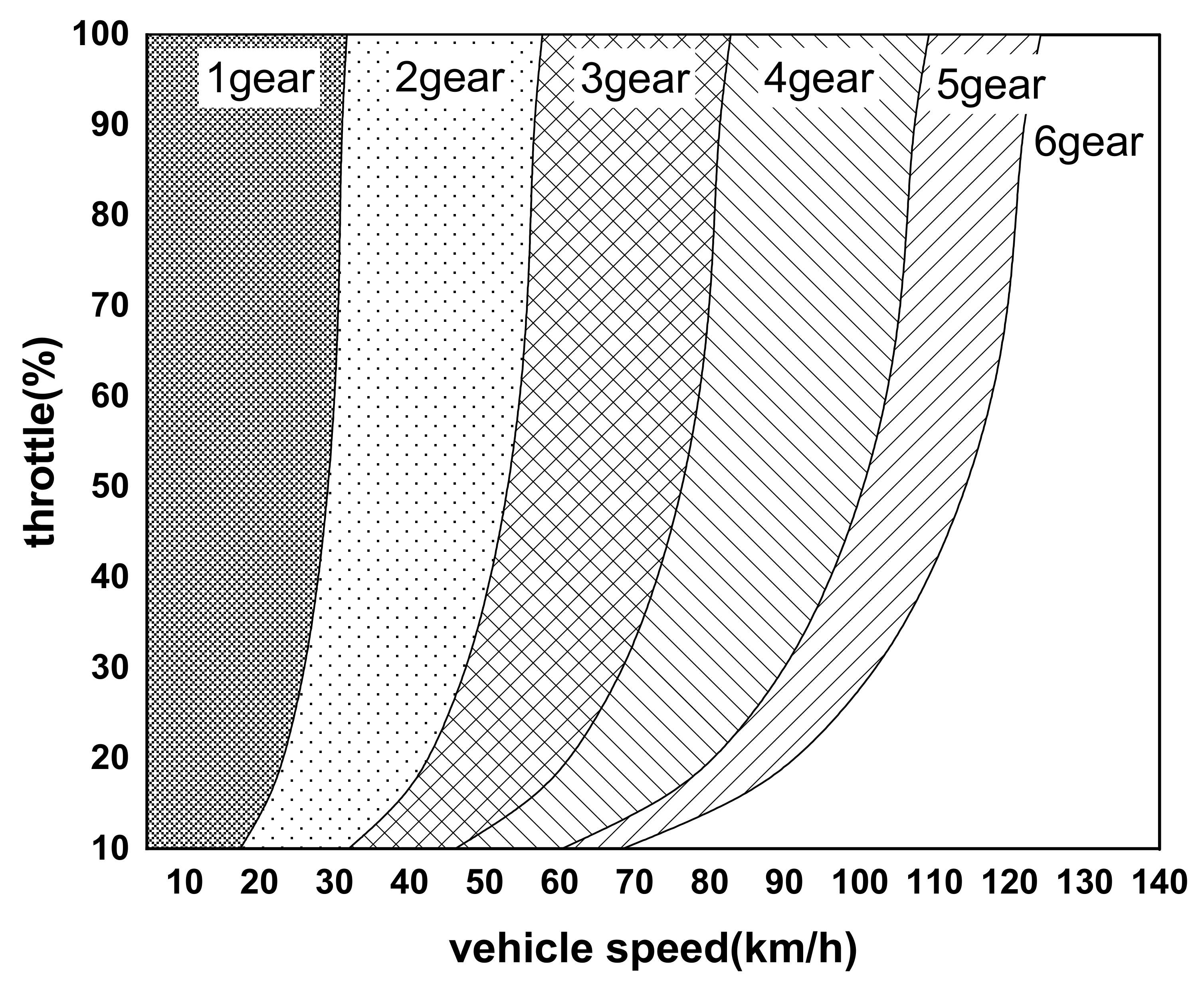
Figure 6.
Fitting fuel consumption diagram of engine.

Figure 7.
Economic upshift point.

Figure 8.
Iterative flow chart of particle swarm optimization.
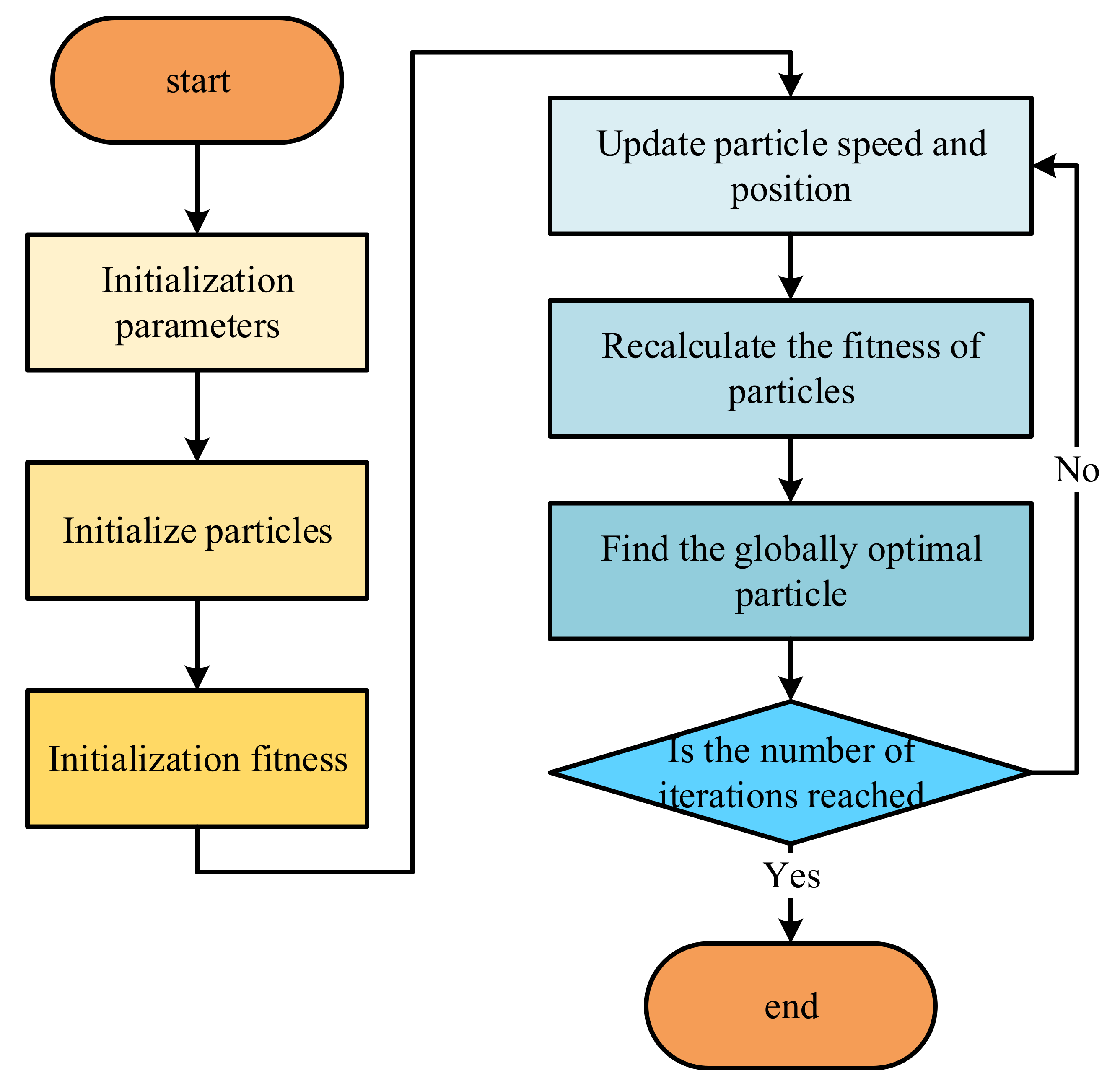
Figure 9.
Iterative diagram of particle swarm optimization algorithm for optimal value of shifting law.
Figure 9.
Iterative diagram of particle swarm optimization algorithm for optimal value of shifting law.
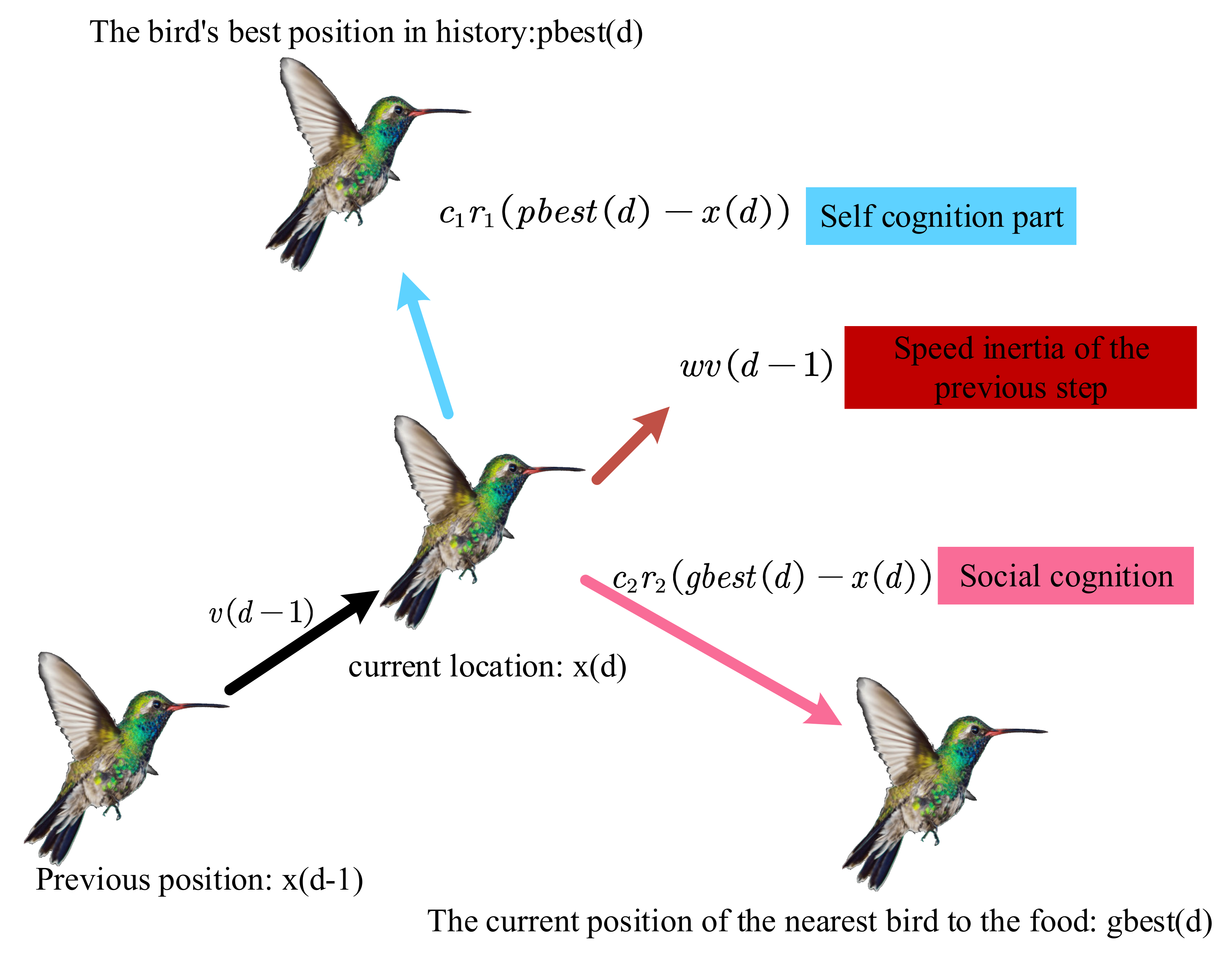
Figure 10.
Optimized upshift point.

Figure 11.
Driver model.
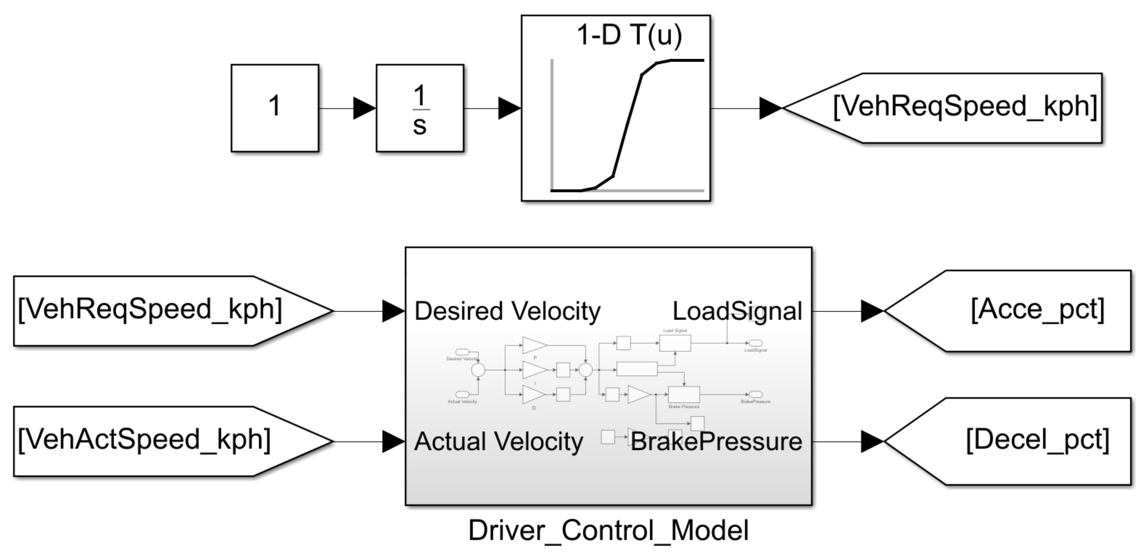
Figure 12.
DCT control strategy.
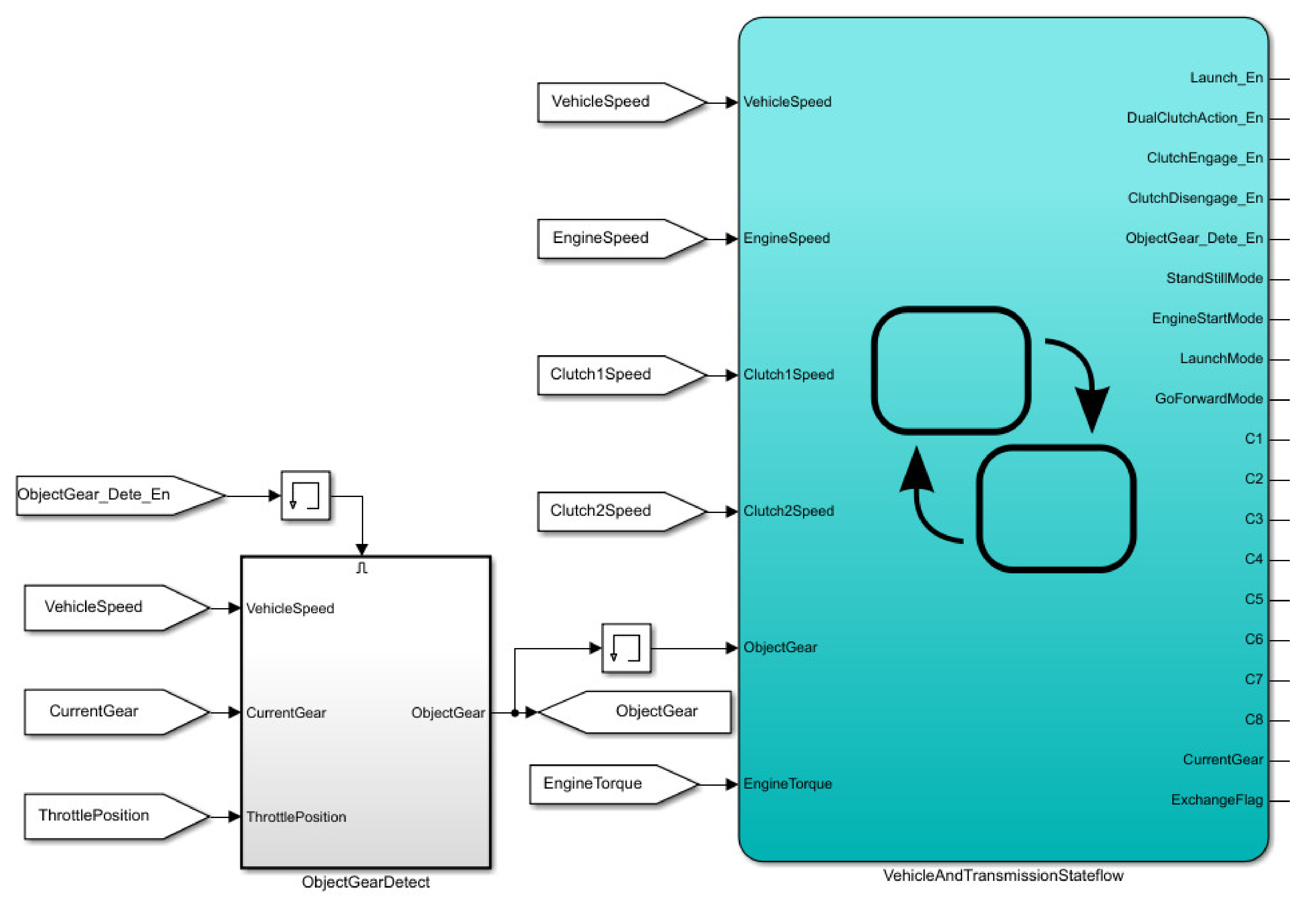
Figure 13.
NEDC and WLTC cycle test conditions.
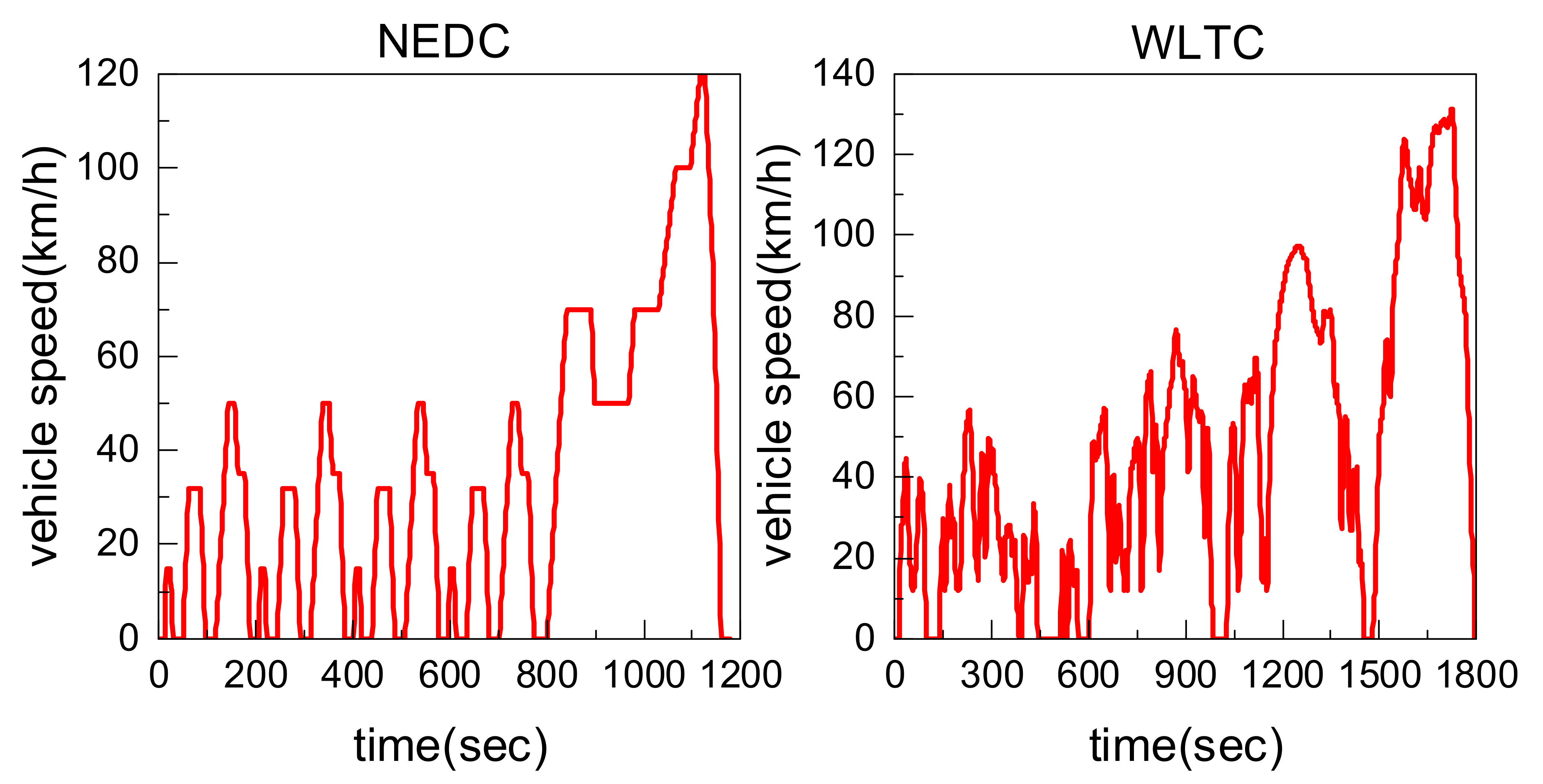
Figure 14.
Actual speed map before and after optimization (NEDC).

Figure 15.
Actual speed map before and after optimization (WLTC).

Figure 16.
Gear selection of different shift strategies under NEDC and WLTC conditions.
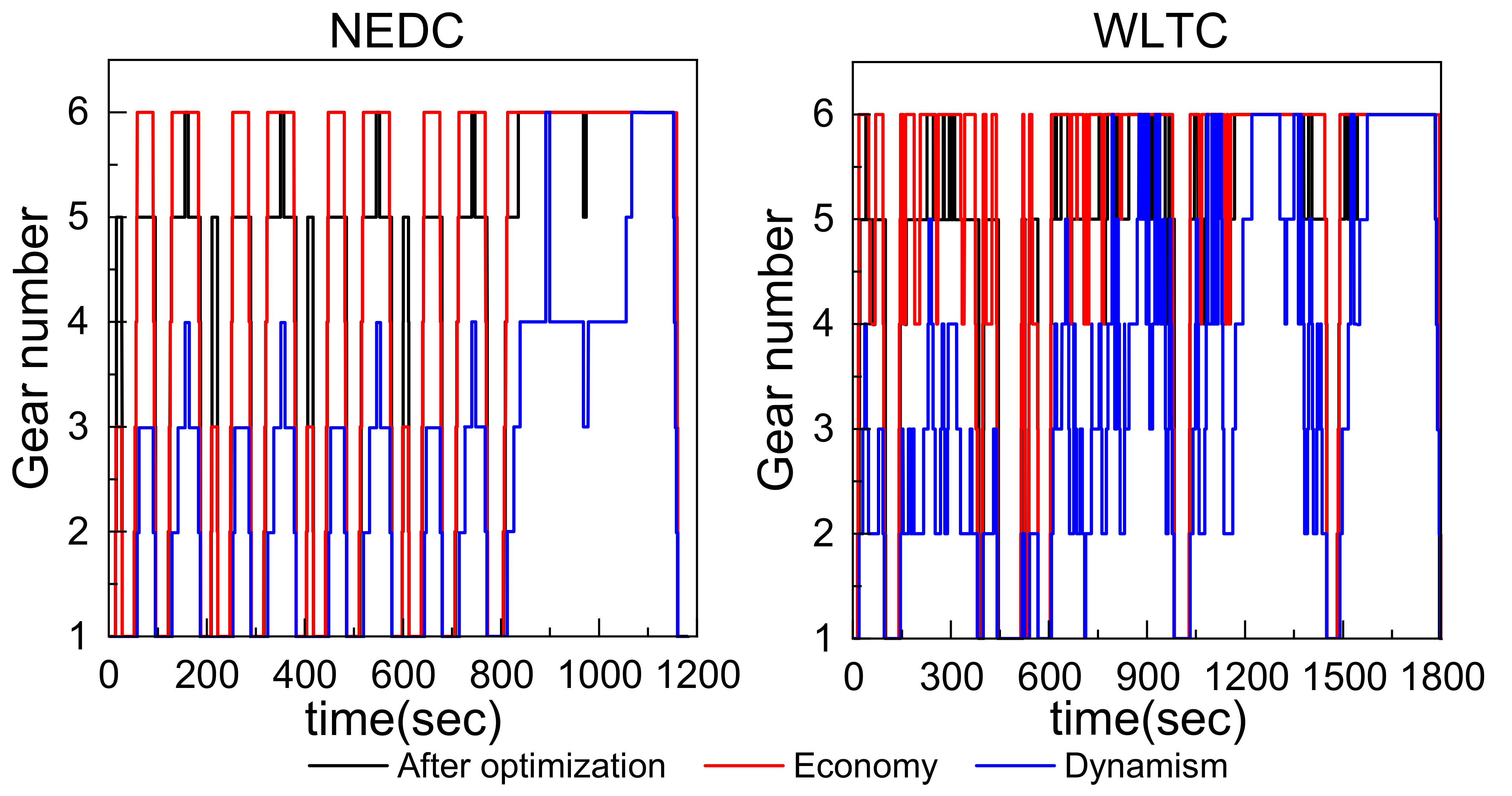
Figure 17.
Fuel consumption of different shift strategies under NEDC and WLTC conditions.
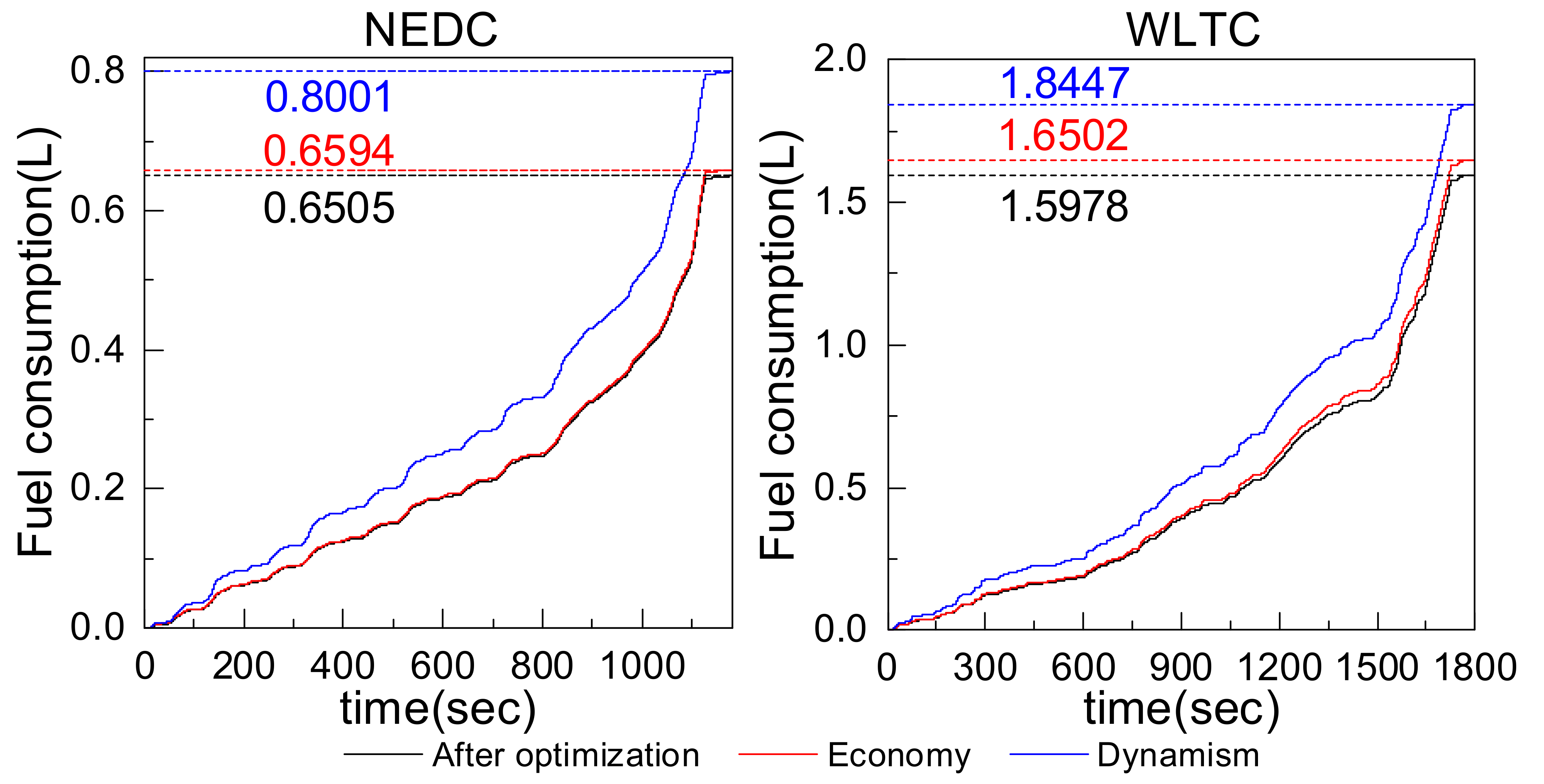
Figure 18.
Dynamic performance verification condition (0–100 km/h).
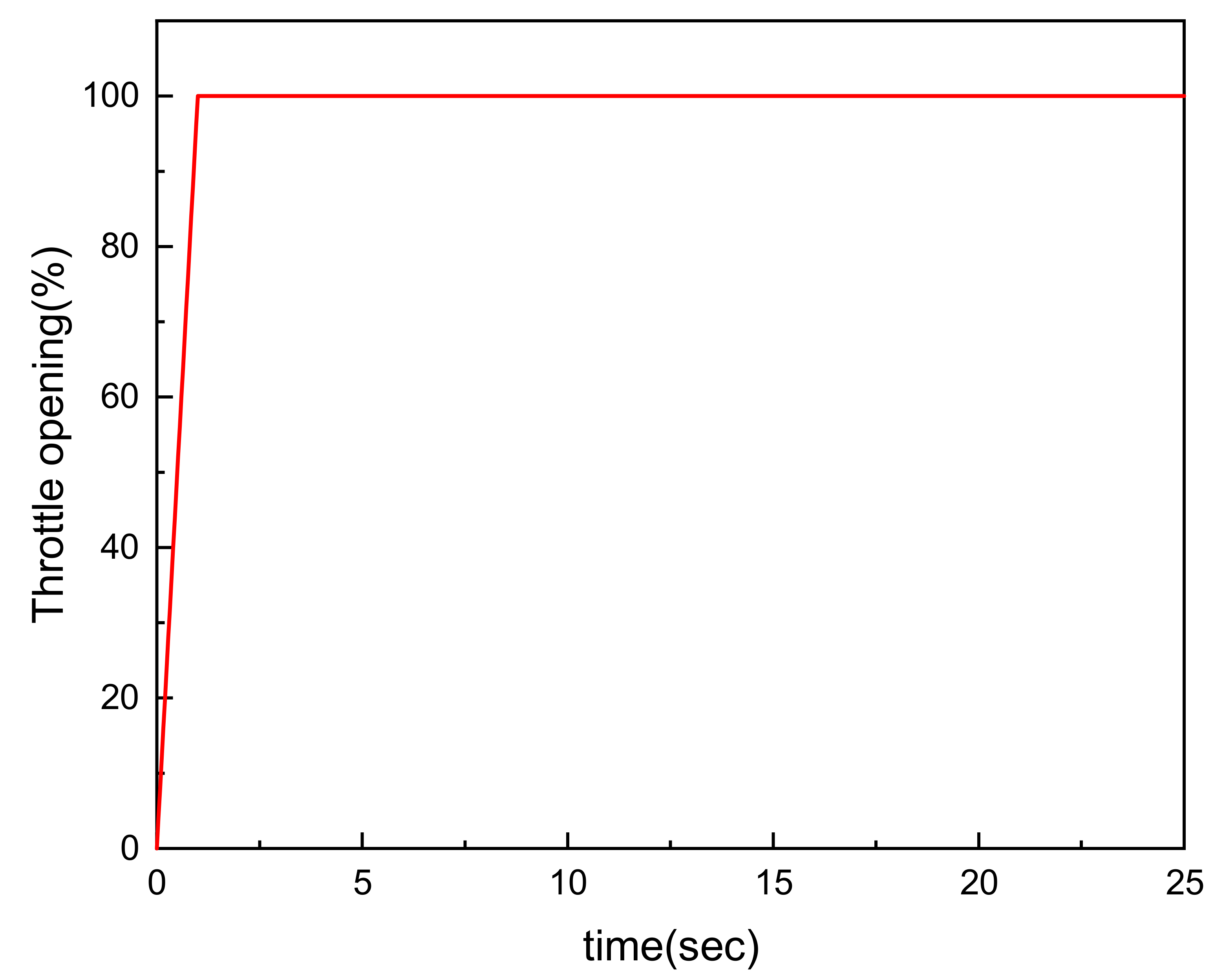
Figure 19.
Gear change of different shift strategies (0–100 km/h).

Figure 20.
Acceleration capability of 0–100 km/h.
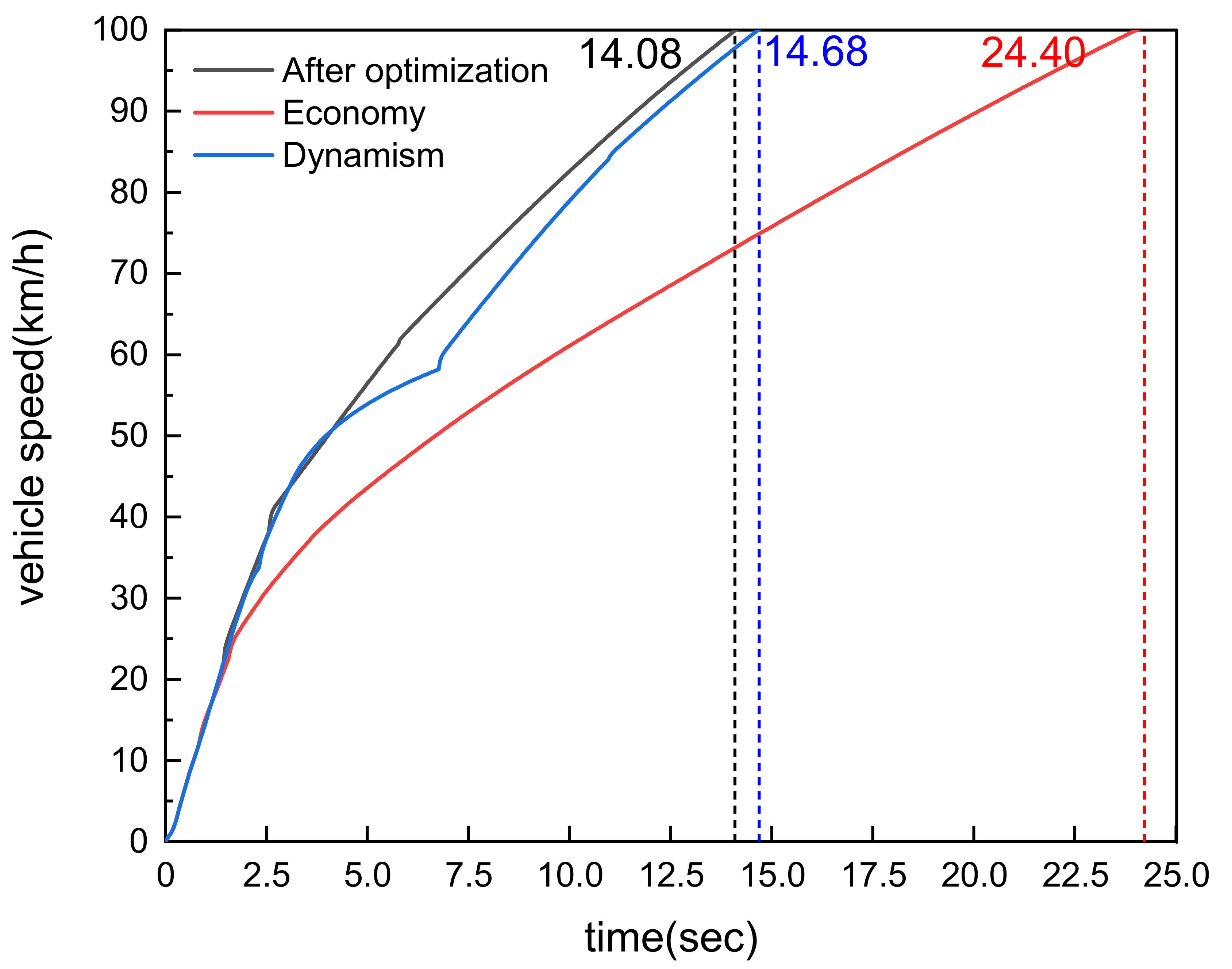
Figure 21.
Acceleration capability of 0–70 km/h.
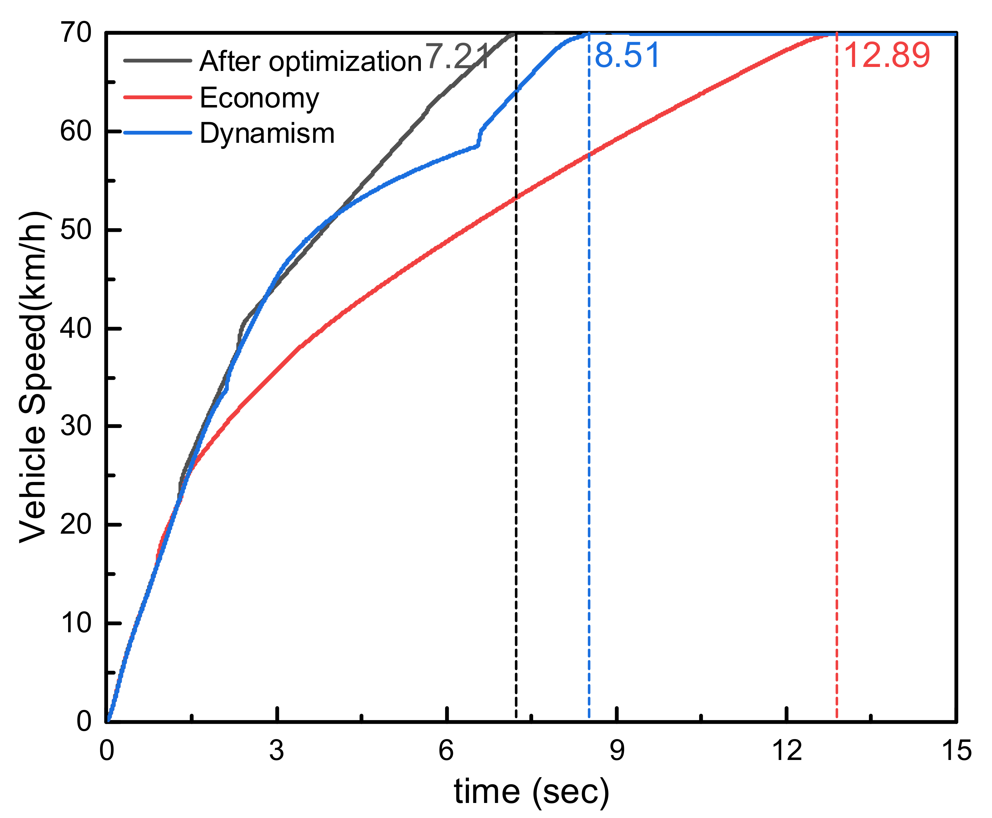
Figure 22.
Acceleration capability of 70–120 km/h.


Table 1.
Main parameters and indicators.
| Type | Name | Index | Units |
|---|---|---|---|
| The vehicle parameters | Weight | 1325 | kg |
| Wheel rolling radius | 0.315 | m | |
| Windward area of vehicles | 1.885 | m2 | |
| Rolling resistance coefficient | 0.015 | 1 | |
| Coefficient of air resistance | 0.36 | 1 | |
| Transmission efficiency | 0.973 | 1 | |
| Ratio of final drive | 3.525 | 1 | |
| Transmission parameter | First gear ratio | 4.83 | 1 |
| Second gear ratio | 3.25 | 1 | |
| Third gear ratio | 1.51 | 1 | |
| Fourth gear ratio | 1.22 | 1 | |
| Fifth gear ratio | 0.885 | 1 | |
| Sixth gear ratio | 0.792 | 1 | |
| Reverse gear ratio | 4.325 | 1 |
Table 2.
Data sheet of power upshift.
| Gear Throttle Opening (%) | 1–2 | 2–3 | 3–4 | 4–5 | 5–6 |
|---|---|---|---|---|---|
| 10 | 17.4568 | 31.9274 | 46.15 | 60.3929 | 68.5103 |
| 15 | 21.101 | 38.721 | 55.95 | 73.378 | 83.28 |
| 20 | 23.391 | 42.89 | 61.9 | 81.28 | 92.2858 |
| 30 | 26.16 | 47.825 | 68.881 | 90.579 | 102.8619 |
| 40 | 27.931 | 50.95 | 73.284 | 96.451 | 109.547 |
| 50 | 29.207 | 53.234 | 76.506 | 100.760 | 114.4549 |
| 60 | 30.08 | 54.844 | 78.787 | 103.822 | 117.947 |
| 70 | 30.581 | 55.792 | 80.139 | 105.649 | 120.0344 |
| 80 | 30.78 | 56.213 | 80.742 | 106.478 | 120.9838 |
| 90 | 30.978 | 56.569 | 81.243 | 107.158 | 121.7612 |
| 100 | 31.66 | 57.752 | 82.903 | 109.352 | 124.2542 |
Table 3.
Data sheet of economic upshift.
| Gear Throttle Opening (%) | 1–2 | 2–3 | 3–4 | 4–5 | 5–6 |
|---|---|---|---|---|---|
| 15 | 4.92 | 8.06 | 11.43 | 14.62 | 16.49 |
| 20 | 6.95 | 11.34 | 16.07 | 20.52 | 23.14 |
| 30 | 7.17 | 11.75 | 16.65 | 21.30 | 24.03 |
| 40 | 7.86 | 12.87 | 18.24 | 23.31 | 26.29 |
| 50 | 8.47 | 13.86 | 19.63 | 25.01 | 28.29 |
| 60 | 9.01 | 14.64 | 20.74 | 26.46 | 29.82 |
| 70 | 9.13 | 14.87 | 21.08 | 26.91 | 30.34 |
| 80 | 9.82 | 15.95 | 22.59 | 28.82 | 32.48 |
| 90 | 11.10 | 18.16 | 25.73 | 32.80 | 37.10 |
| 100 | 12.18 | 19.72 | 27.93 | 35.60 | 40.12 |
Table 4.
Comparison table of dynamic performance verification.
| Working Condition | NEDC | Reduced Proportion after Optimization | WLTC | Reduced Proportion after Optimization |
|---|---|---|---|---|
| Total fuel consumption of dynamic shift strategy (L) | 0.8001 | 18.70% | 1.8447 | 13.38% |
| Total fuel consumption of economical shift strategy (L) | 0.6594 | 1.37% | 1.6502 | 3.18% |
| Total fuel consumption of optimized shift strategy (L) | 0.6505 | 0.00% | 1.5978 | 0.00% |
Table 5.
Comparison table of economic verification of 0–100 km/h.
| Working Condition | 0–100 km/h | Reduced Proportion after Optimization |
|---|---|---|
| Total time for dynamic shift strategy (s) | 14.68 | 4.087% |
| Total time for economic shift strategy (s) | 24.40 | 42.30% |
| Total optimized shift strategy time (s) | 14.08 | 0.00% |
Table 6.
Comparison table of economic verification of 0–70 km/h.
| Working Condition | 0–70 km/h | Reduced Proportion after Optimization |
|---|---|---|
| Total time for dynamic shift strategy (s) | 8.51 | 15.28% |
| Total time for economic shift strategy (s) | 12.89 | 44.07% |
| Total optimized shift strategy time (s) | 7.21 | 0.00% |
Table 7.
Comparison table of economic verification of 70–120 km/h.
| Working Condition | 70–120 km/h | Reduced Proportion after Optimization |
|---|---|---|
| Total time for dynamic shift strategy (s) | 13.69 | −10.70% |
| Total time for economic shift strategy (s) | 20.58 | 25.51% |
| Total optimized shift strategy time (s) | 15.33 | 0.00% |
Publisher’s Note: MDPI stays neutral with regard to jurisdictional claims in published maps and institutional affiliations. |
© 2021 by the authors. Licensee MDPI, Basel, Switzerland. This article is an open access article distributed under the terms and conditions of the Creative Commons Attribution (CC BY) license (https://creativecommons.org/licenses/by/4.0/).
Share and Cite
MDPI and ACS Style
Zhang, H.; Yang, X.; Sun, X.; Liang, J. Optimal Design of Shift Point Strategy for DCT Based on Particle Swarm Optimization. Machines 2021, 9, 196. https://doi.org/10.3390/machines9090196
AMA Style
Zhang H, Yang X, Sun X, Liang J. Optimal Design of Shift Point Strategy for DCT Based on Particle Swarm Optimization. Machines. 2021; 9(9):196. https://doi.org/10.3390/machines9090196
Chicago/Turabian StyleZhang, Houzhong, Xiangtian Yang, Xiaoqiang Sun, and Jiasheng Liang. 2021. "Optimal Design of Shift Point Strategy for DCT Based on Particle Swarm Optimization" Machines 9, no. 9: 196. https://doi.org/10.3390/machines9090196
Note that from the first issue of 2016, this journal uses article numbers instead of page numbers. See further details here.