Abstract
Blazars show rapid and high amplitude variability. It is interesting to question what kind of process the variability corresponds to. Maybe it is a result of the instability of the accretion flows. In this work, Fermi daily light curves of 130 sources are analyzed, and the distributions of daily variability are compared by using a Kolmogorov–Smirnov (K-S) test. The results can be summarized as follows:(1) in most cases, the distributions are not Gaussian; (2) some pairs of the distributions are similar.
1. Introduction
Blazars represent an extreme subclass of AGN (Active Galactic Nuclei). It is believed that the jet of the blazar flows along the line of our sight. The blazar model consists of a supermassive black hole in the center, an accretion disk and a torus around it, and a relativistic jet in the direction of the poles. From observation, blazars show rapid and significant variability, high polarization of radiation, and superluminal motion and other changes with time.
A vast amount of observational data has been obtained about the variability of blazars. Many cases of periodic variability have been found from the light curves of blazars (see [1,2,3,4,5,6,7] and references therein). From another point of view, the data also shows that blazar light curves are similar to the “red noise” in the frequency domain (see [8,9,10] and reference therein). Therefore, what type of “red noise” is it?
2. Data and Analysis
2.1. Data and Preprocessing
The analyses of daily light curves here were retrieved from the on-line database of the (LAT) 1. Data for a total of 130 Fermi sources were obtained.
Commonly, fluxes of Fermi sources are highly variable. Here, was used to denote the flux at time t. Because the time interval of the flux is usually one day, the daily variability of flux can be calculated by the formula
Here is the daily variability of the flux, and N is the number of observational data.
Then, the mean value μ and the standard deviation s of can be obtained by the two formulas below,
Next, was subtracted by μ and divided by s to normalize,
Here, is the normalized daily variability of flux, with a mean of 0 and a variation of 1.
2.2. Test and Pairwise Comparison
When values of have been obtained, the Kolmogorov–Smirnov test (K-S test) can be used to test whether the distribution of is similar to a Gaussian distribution. First, the cumulative distribution function (CDF) of should be calculated and is denoted by .
is a function giving the fraction of observations of the measured variable that are less than or equal to x. is constant between consecutive points, with a constant value of added at each (See Figure 1).
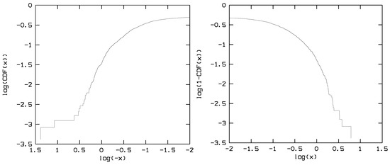
Figure 1.
The double logarithmic graph of the cumulative distribution function (CDF). The left is the plot of the negative data set of , the right is the plot of the negative data set of .
For each source of the sample, the K-S test was used to make a comparison between the distribution of and a Gaussian distribution. The K-S statistic D and the significance level p of the equivalence can be obtained. For example, for PKS 2255-282, D is 0.142 and the significance p is ; for 3C 446, D is 0.136 and the significance p is ; for PKS 2320-035, D is 0.192 and the significance p is ; for CGRaBS J0211+1051, D is 0.190, and the significance p is less than . The double logarithmic graphs of CDF curves are shown in the bottom panel of Figure 2. The results indicate that the variability of the Fermi light curve of these objects is not similar to Gaussian noise.
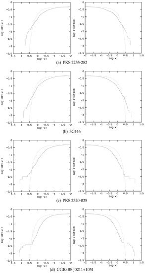
Figure 2.
Double logarithmic graphs of the cumulative probability distributions of PKS 2255-282, 3C446, PKS 2320-035, and CGRaBS J0211+1051. The solid line is the cumulative probability distribution of the source, the dotted line is the cumulative probability distribution of a Gaussian distribution. For PKS 2255-282, the distribution of and the Gaussian distribution are similar with , for 3C 446, they are similar with , for PKS 2320-035, they are similar with , and for CGRaBS J0211+1051, they are similar with .
Next, a K-S test was done for the normalized daily light variability for any pair of sources. We show the two best pairs of sources. Figure 3 shows the double logarithmic graphs of CDFs of PKS 2255-282 and 3C446. The significance of the equivalence for the distributions of these two objects is .
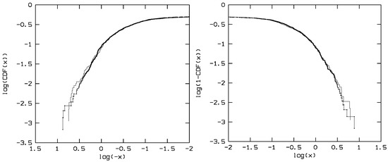
Figure 3.
Double logarithmic graphs of CDFs of PKS 2255-282 and 3C446. The thin line is the CDF of PKS 2255-282, the thick line is the CDF of 3C446. The distributions of PKS 2255-282 and 3C446 are similar at the 94.3 percent level.
The double logarithmic graphs of CDFs of PKS 2320-035 and CGRaBS J0211+1051 are plotted in Figure 4, which shows that the equivalence is at the 94.9 percent level according to the K-S test.
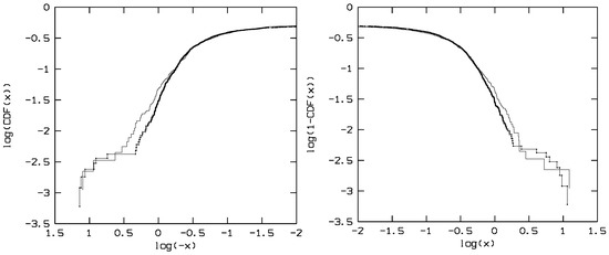
Figure 4.
Double logarithmic graphs of CDFs of PKS 2320-035 and CGRaBS J0211+1051. The thin line is the CDF of PKS 2320-035, the thick line is the CDF of CGRaBS J0211+1051. The distributions of PKS 2320-035 and CGRaBS J0211+1051 are similar at the 94.9 percent level.
Based on the former results, the cumulative probability distribution of most sources is not Gaussian. So we examine the greatest deviations between the two wings of the distribution as well. To do this, we consider those measured data which belong to the negative and the positive of the data set of . could be approximated by a power-law function, respectively,
denotes the exponent of the distribution function for the positive variability, and denotes that for the negative. and can be obtained by using linear regression in the double logarithmic graph of the CDF. We show an example in Figure 5. A total of 130 sources are included, so 130 and have been derived. We plot all the and in Figure 6.
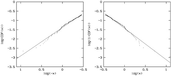
Figure 5.
The left plot is the double logarithmic graph of the CDF of the negative of the data set of and the solid line represents the best fitting result for the negative of the data set of . The right plot is the double logarithmic graph of the CDF of the positive of the data set of , and the solid line represents the best fitting result for the positive of the data set of .
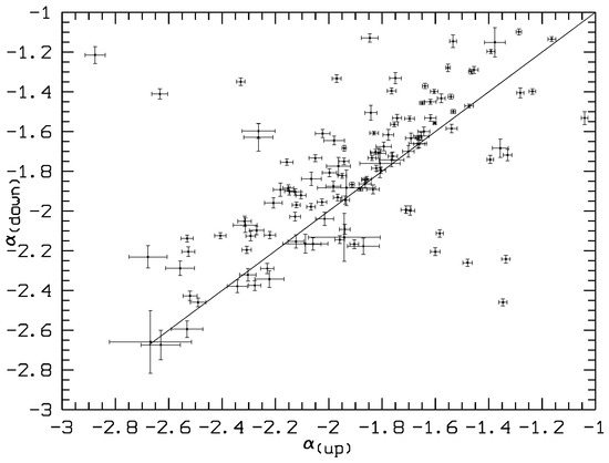
Figure 6.
Plot of versus . The solid line indicates the straight line with .
3. Discussion
From the observations, we find that the light curves of the blazars we studied are extremely variable. The variable mode is usually of a “red noise” nature in the frequency domain. A simple model of the “red noise” is Brownian or random walk noise, which can be produced by integrating the white noise. If the light curves of the blazars were produced by a similar process, the daily variability should be similar to a Gaussian distribution. The K-S was used to test for the Fermi light curve of the blazar. The test results show that the distribution of the daily variation of gamma-ray emission is not equivalent to a Gaussian distribution. The variability of gamma-ray emission of some Fermi blazars should not be considered as being produced only by integrating a finite number of random emission events. Perhaps it is connected with some internal physical mechanism instead.
When we conduct the K-S test for the daily variability distributions of any pair of sources, the distributions of some pairs of sources are found to be very similar. Additionally, their distributions are different from Gaussian distributions. Maybe some similar physical mechanism can produce these variations.
Since the distribution of daily variability does not follow a Gaussian distribution, some parameters of the distribution should be checked. In Figure 6, most of the data points are located on the top of the line . This means that the distribution of negative variability is slightly flatter than that of positive variability. This possibility indicates that there are more extreme events in the decay process than in the ascending process.
Acknowledgments
This work is partially supported by the National Natural Science Foundation of China (NSFC U1531245, U1431112, 11203007, 11403006, 10633010, 11173009), the Innovation Foundation of Guangzhou University (IFGZ), Guangdong Province Universities and Colleges Pearl River Scholar Funded Scheme(GDUPS)(2009), Yangcheng Scholar Funded Scheme(10A027S), and support for Astrophysics Key Subjects of Guangdong Province and Guangzhou City. The Abastumani team acknowledges financial support of the project FR/639/6-320/12 by the Shota Rustaveli National Science Foundation under contract 31/76. This work was presented in ”Blazars through Sharp Multi-Wavelength Eyes”, Malaga (Spain), 30 May–3 June 2016. This research has made use of data obtained through the High Energy Astrophysics Science Archive Research Center Online Service, provided by the NASA/Goddard Space Flight Center.
Author Contributions
Cai Wei and Yi Liu are responsible for the writing and the motivation of the paper; Junhui Fan is responsible for some discussions.
Conflicts of Interest
The authors declare no conflict of interest.
References
- Fan, J.H.; Xie, G.Z.; Lin, R.G.; Qin, Y.P.; Li, K.H.; Zhang, X. The long-term variability of BL Lac object PKS 0735+178. Astron. Astrophys. Supp. 1997, 125, 525–528. [Google Scholar] [CrossRef]
- Fan, J.H.; Xie, G.Z.; Pecontal, E.; Pecontal, A.; Copin, Y. Historic light curve and long-term optical variation of BL Lacertae 2200+420. Astrophys. J. 1998, 507, 173–178. [Google Scholar] [CrossRef]
- Fan, J.H.; Xie, G.Z.; Adam, G.; Copin, Y.; Lin, R.G.; Bai, J.M.; Qin, Y.P. Long-term Variation of AGNs. BL Lac Phenom. 1999, 159, 99. [Google Scholar]
- Fan, J.H.; Lin, R.G. Optical Variability and Periodicity Analysis for Blazars. I. Light Curves for Radio-selected BL Lacertae Objects. Astrophys. J. 2000, 537, 101–122. [Google Scholar] [CrossRef]
- Fan, J.H.; Lin, R.G.; Xie, G.Z.; Zhang, L.; Mei, D.C.; Su, C.Y.; Peng, Z.M. Optical periodicity analysis for radio selected BL Lacertae objects (RBLs). Astron. Astrophys. 2002, 381, 1–5. [Google Scholar] [CrossRef]
- Fan, J.H. Optical variability of Blazars. Chin. J Astron. Astrophys. 2005, 5, 213–223. [Google Scholar] [CrossRef]
- Fan, J.H.; Liu, Y.; Yuan, Y.H.; Hua, T.X.; Wang, H.G.; Wang, Y.X.; Yang, J.H.; Gupta, A.C.; Li, J.; Zhou, J.L.; et al. Radio variability properties for radio sources. Astron. Astrophys. 2007, 62, 547–552. [Google Scholar] [CrossRef]
- Watson, M.G.; Pounds, K.A.; Elvis, M. Low-frequency divergent X-ray variability in the Seyfert galaxy NGC4051. Nature 1987, 325, 694–696. [Google Scholar]
- Chatterjee, R.; Jorstad, S.G.; Marscher, A.P.; Oh, H.; McHardy, I.M.; Aller, M.F.; Aller, H.D.; Balonek, T.J.; Miller, H.R.; Ryle, W.T.; Tosti, G. Correlated multi-wave band variability in the blazar 3C 279 from 1996 to 2007. Astrophys. J. 2008, 689, 79–94. [Google Scholar] [CrossRef]
- Kataoka, J.; Takahashi, T.; Wagner, S.J.; Iyomoto, N.; Edwards, P.G.; Hayashida, K.; Inoue, S.; Madejski, G.M.; Takahara, F.; Tanihata, C.; Kawai, N. Characteristic x-ray variability of TeV blazars: Probing the link between the jet and the central engine. Astrophys. J. 2001, 560, 659–674. [Google Scholar] [CrossRef]
© 2017 by the authors. Licensee MDPI, Basel, Switzerland. This article is an open access article distributed under the terms and conditions of the Creative Commons Attribution (CC BY) license ( http://creativecommons.org/licenses/by/4.0/).