Article

Relativistic Jet Simulations of the Weibel Instability in the Slab Model to Cylindrical Jets with Helical Magnetic Fields

1
Department of Physics, Chemistry and Mathematics, Alabama A&M University, Normal, AL 35762, USA
2
Institute for Theoretical Physics, Goethe University, D-60438 Frankfurt am Main, Germany
3
Instituto de Astrofísica de Andalucía, CSIC, Apartado 3004, 18080 Granada, Spain
4
Institute of Space Science, Atomistilor 409, RO-077125 Bucharest-Magurele, Romania
5
Department of Physics and Astronomy, University of Gent, Proeftuinstraat 86, B-9000 Gent, Belgium
6
Space Sciences & Technologies for Astrophysics Research (STAR) Institute Universite de Liege, Sart Tilman, 4000 Liège, Belgium
7
Institute of Nuclear Physics PAN, ul. Radzikowskiego 152, 31-342 Kraków, Poland
8
Institut fur Physik und Astronomie, Universität Potsdam, 14476 Potsdam-Golm, Germany
9
DESY, Platanenallee 6, 15738 Zeuthen, Germany
10
Laboratory for the Universe and THeory, Observatore de Paris-Meudon, 5 Place Jules Jansen, 92195 Meudon CEDEX, France
11
Max-Planck-Institut für Radioastronomie, Auf dem Hügel 69, D-53121 Bonn, Germany
12
Department of Physics and Astronomy, Clemson University, Clemson, SC 29634, USA
*
Author to whom correspondence should be addressed.
Galaxies 2019, 7(1), 29; https://doi.org/10.3390/galaxies7010029
Submission received: 14 November 2018 / Revised: 17 January 2019 / Accepted: 21 January 2019 / Published: 30 January 2019
(This article belongs to the Special Issue Cosmic Plasmas and Electromagnetic Phenomena)

Abstract

:
The particle-in-cell (PIC) method was developed to investigate microscopic phenomena, and with the advances in computing power, newly developed codes have been used for several fields, such as astrophysical, magnetospheric, and solar plasmas. PIC applications have grown extensively, with large computing powers available on supercomputers such as Pleiades and Blue Waters in the US. For astrophysical plasma research, PIC methods have been utilized for several topics, such as reconnection, pulsar dynamics, non-relativistic shocks, relativistic shocks, and relativistic jets. PIC simulations of relativistic jets have been reviewed with emphasis placed on the physics involved in the simulations. This review summarizes PIC simulations, starting with the Weibel instability in slab models of jets, and then focuses on global jet evolution in helical magnetic field geometry. In particular, we address kinetic Kelvin-Helmholtz instabilities and mushroom instabilities.

1. Introduction

Relativistic jets are collimated outflows of ionized matter powered by black holes. Sites for such jets include the collapse of the core of a massive star forming a neutron star or a black hole, the merger of binary neutron stars, supermassive black holes associated with active galactic nuclei (AGN), gamma-ray bursts (GRBs), and pulsars (e.g., [1]). GRBs and blazars produce the brightest electromagnetic phenomena in the universe (e.g., [2]). Despite extensive observational, theoretical, and simulation studies, the understanding of their formation, their interaction with interstellar mediums, and consequently, their observable properties, such as spectra, variability, and polarization (e.g., [3]), remain quite limited.
Astrophysical jets are ubiquitous and exhibit a wide range of plasma phenomena, such as propagation in the interstellar medium, generation/decay of magnetic fields, magnetic reconnection, and turbulence. In these dynamic environments, particle acceleration may be able to achieve the highest level of energies observed in cosmic rays. Many of the processes that determine the evolution of global relativistic jets are very complex, and they occur on small spatial and short temporal scales associated with plasma kinetic effects. It is especially challenging to integrate microscopic physics into global, large-scale dynamics, which is crucial to understand the full dynamics of the jets. Kinetic plasma simulations are traditionally performed using particle-in-cell (PIC) codes, with the intent of addressing particle acceleration and kinetic magnetic reconnection, which cannot be investigated with fluid models (i.e., relativistic magnetohydrodynamic (RMHD) simulations). In particular, PIC simulations indicate that particle acceleration occurs due to kinetic instabilities, such as electron and ion Weibel instabilities (e.g., [4,5,6,7,8,9,10,11,12,13,14,15,16,17,18,19,20,21,22,23,24,25,26]).
In general, these simulations confirm that the Weibel instability is dominant among kinetic instabilities develped in weak or nonmagnetized plasma [27]. These instabilities, which develop in relativistic outflows, also lead to multiple shock structures. Dynamically changing current filaments and magnetic fields (e.g., [28]) accelerate electrons (e.g., [12]) and cosmic rays, which affect the pre-shock medium [29]. In order to model a shock, a relativistic plasma flow is injected from one end of the computational grid and reflected from a boundary at the opposite end. Such simulations are performed by the following: 1D simulations by [30,31], 2D simulations by (e.g., [14,15,19,25,26,32]), and 3D simulations by [33,34]. This method creates two identical counter-streaming beams which collide and interact. This approach also simplifies the numerical method, but leads to the drawbackwhere only one forward-moving shock (FS) is generated. In these settings, the backward (reverse) shock (RS) is indistinguishable from FS. There is another method where a jet is injected into an ambient plasma where FS and RS shock structures are fully modelled. Contact discontinuity (CD) is generated due to deceleration of the jet flow by the ambient plasma. The CD is the location where the electromagnetic field, the velocity of the jet, and the ambient plasmas are similar, but the density changes. FS and RS propagate away from the CD into the jet and ambient plasmas (in the CD frame) [18,21,22,23]. Ardaneh et al. [22] showed that FS, RS, and CD separate the jet and ambient plasma into four regions: (1) the unshocked ambient, (2) shocked ambient, (3) shocked jet, and (4) unshocked jet. In this way, the jet-to-ambient density ratio was selected as the appropriate plasma conditions of AGN and GRB jets. The shock formation processes can be investigated temporally and spatially. A leading and trailing shock system develops with strong electromagnetic fields accompanying the trailing shock. PIC simulations where jets are reflected at the simulation boundary were reviewed, including the generation of high-energy particles, by [35].
In this review, we briefly summarize our previous studies from the slab jet case to the global cylindrical jet case and present new three-dimensional simulation results for an electron-positron jet injected into an electron-positron plasma using a long simulation grid in the jet-propagation direction. We also present the results of a new study of global relativistic jets containing helical magnetic fields. The global simulation results, including velocity shears (this time) using a small simulation system, validate the use of the simulation code for the research project.

2. PIC Simulations in a Slab Model

It is natural to start to perform PIC simulations in a slab model where jets are injected into the whole simulation system. Since we use the periodic boundary conditions in the transverse direction to the jets, we are simulating a part of the jets without taking into account the boundary between the jets and the ambient plasmas. The instabilities generated between jets and ambient plasmas are described later.

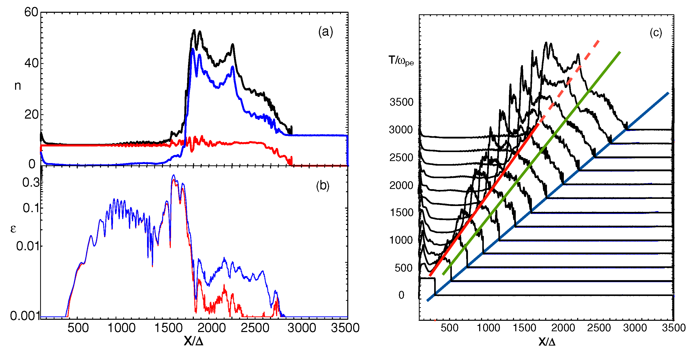
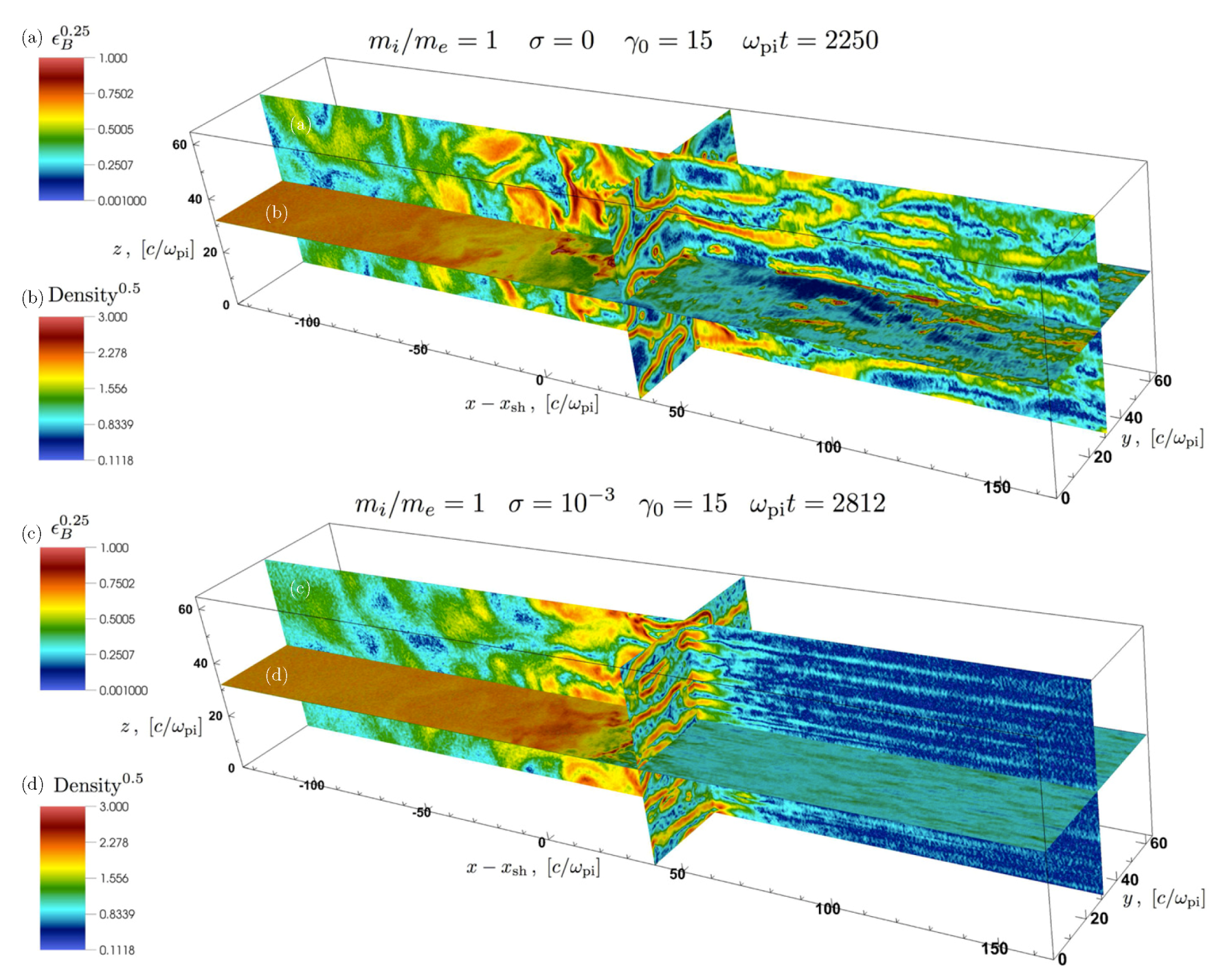
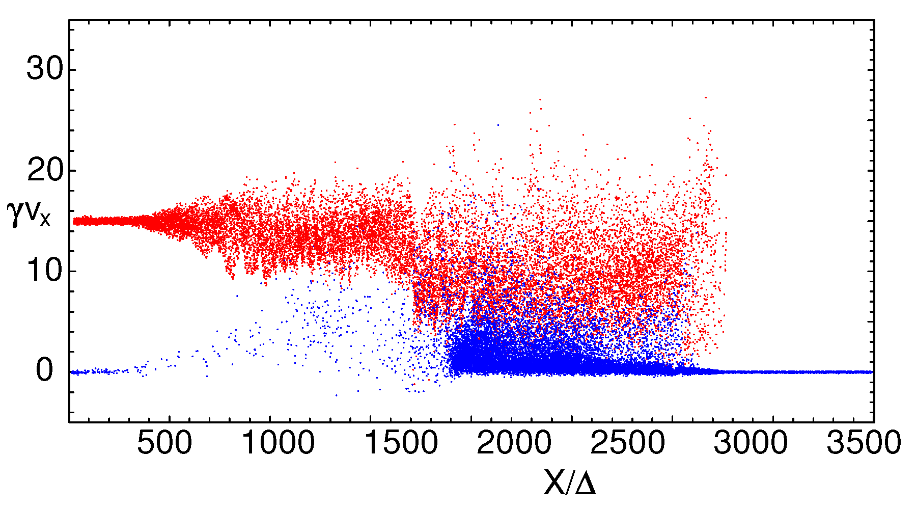
2.1. Simulation of the Weibel Instability

The Weibel instability is a plasma instability which occurs in homogeneous or nearly homogeneous plasmas, where an anisotropy in the momentum (velocity) space exists [27]. The Weibel instability is often referred to as a filamentation instability [36].
The mechanisms of Weibel instability growth are explained as the following: Suppose a field B = B z cos k y is spontaneously generated by thermal fluctuation. Here, k is a wave number, the x , y , and z are the coordinates, and electrons travel along the x-direction. The Lorentz force ( e v × B ) then bends the electron trajectories (travelling along the x-direction) along the y-direction, resulting in congregation of the electrons. The resultant current j = e n v e sheets (filaments) create a magnetic field, which enhances the original field and thus grows perturbation [28]. The Weibel instability is also common in astrophysical plasmas, such as collisionless shock formation in jets, supernova remnants, and GRBs.

2.1.1. Simulation Settings

The code used in this study is an MPI-based parallel version of the relativistic particle-in-cell (RPIC) code, TRISTAN [5,37,38]. The simulations have been performed using a grid with ( L x , L y , L z ) = ( 4005 , 131 , 131 ) cells and a total of ∼1 billion particles (12 particles/cell/species for the ambient plasma) in the active grid. The electron skin depth is λ s = c / ω pe = 10.0 Δ , where c = 1 is the speed of light and ω pe = ( e 2 n a / ϵ 0 m e ) 1 / 2 is the electron plasma frequency, and the electron Debye length λ D is half of the cell size, Δ . This computational system length is six times longer than that used in the previous simulations [12,39]. The jet-electron number density in the simulation reference frame is 0.676 n a , where n a is the ambient electron density, and the jet Lorentz factor is γ jt = 15 . The jet-electron/positron thermal velocity is v j , th = 0.014 c in the jet reference frame. The electron/positron thermal velocity in the ambient plasma is v a , th = 0.05 c . As in our previous work (e.g., [12]), the jet is injected in a plane across the computational grid located at x = 25 Δ in order to eliminate artificial effects associated with the boundary at x = x min . Radiating boundary conditions are used on the planes at x = x min and x = x max and periodic boundary conditions on all transverse boundaries [37]. The jet makes contact with the ambient plasma at a two-dimensional interface spanning the whole computational domain in the y z plane. In this way, only a small portion of whole jets is studied; that is, the simulation includes the spatial development of nonlinear saturation and dissipation from the injection point to the jet front composed of the fastest-moving jet particles. Therefore, the boundary between jets and ambient plasma is not taken into account, which will be described later.

2.1.2. Simulation Results

Figure 1a,b shows the average (in the y z plane) of (a) the jet (red), the ambient (blue), and the total (black) electron density, and (b) the electromagnetic field energy divided by the total jet kinetic energy ( E t j = i = e , p m i c 2 ( γ jt 1 ) ) at t = 3250 ω p e 1 . Here, “e” and “p” denote the electron and positron. Positron density profiles are similar to the electron profiles, as both particles have the same mass. However, for the electron-ion jets, the densities of the electrons and the ions are slightly different, giving rise to double layers in the plasma [21,22,23]. As a result, ambient particles are dragged by the motion of the jet particles up to x / Δ ∼500. By t = 3250 ω p e 1 , the ambient density has evolved into a two-step plateau behind the jet front, which is similar to the electron-ion jet cases [21,22,23]. The maximum density in this shocked region is about three times the initial ambient density. The jet-particle density remains nearly constant up to near the front of the jet. Careful comparisons reveal the differences between the pair jets and the electron-ion jets [21,22,23]. The differences arise due to the double layers generated in the trailing and leading edges in the electron-ion jets.
The growth of the Weibel instability creates current filaments and strong electromagnetic fields in the trailing shock region. Since the nonlinear stage is formed in this simulation, the electromagnetic fields are about four times larger than those seen previously in simulations with a much shorter grid system ( L x = 640 Δ ). At the simulation time t = 3250 ω p e 1 , the electromagnetic fields have the highest intensity at x / Δ ∼1700, which then declines by about one order of magnitude beyond x / Δ = 2300 in the shocked region [12,39].
Figure 1c shows the total electron density plotted at time intervals of δ t = 250 ω pe 1 . The jet front propagates with the initial jet speed (≤c). Since anomalous resistivity exists in PIC simulations, sharp RMHD-simulation shock surfaces are not generated (e.g., [40]). A leading shock region (where the linear density increases) moves with a speed between that of the fastest moving jet particles ≤c and a predicted CD value of ∼ 0.76 c . A CD region consisting of mixed ambient and jet particles moves at a speed which is between ∼ 0.76 c , and the trailing density jump speed ∼ 0.56 c . The modest density increase just behind the large trailing density jump should be taken note of. Similar shock structures and their velocities for the electron-ion jets are discussed in [21,22,23].
It is important to show the differences between the reflection and the injection models. The shock is set up by reflecting a cold “upstream” flow from a conducting wall located at x = 0 (Figure 1). The interaction between the incoming beam (that propagates along x ) and the reflected beam triggers the formation of a shock, which moves away from the wall along + x [33]. This setup is equivalent to the head-on collision of two identical plasma shells, which would form a forward and reverse shock and contact discontinuity as an injection scheme. However, the forward and reverse shocks are not distinguished as in the injection scheme. Furthermore, the conducting wall corresponds to the contact discontinuity. The simulation is performed in the “wall” frame, where the “downstream” plasma behind the shock is stationary—and on the contrary, in the injection scheme, FS, RS, and CD are moving in the same direction.
In 3D, periodic boundary conditions are employed both in y- and in z-directions. Each computational cell is initialized with four particles (two per species) in 2D and two particles (one per species) in 3D. They have performed limited number of experiments with a larger number of particles per cell (up to eight per species in 2D), though essentially obtaining the same results.
Their 3D structure is shown in Figure 2, for a relativistic electron-positron shock with magnetization σ = B 2 / n e m e γ jt c 2 = 0 (top panel) and σ = 10 3 (bottom panel). The background magnetic field B 0 is initially set along the z-direction, in the same way as for our 2D simulations. The y z slice of the magnetic energy fraction in Figure 2c shows that for σ = 10 3 , the magnetic field ahead of the shock is primarily organized in pancakes stretched in the direction orthogonal to the background magnetic field (i.e., along y). This can be easily understood, considering that the Weibel instability is seeded by focusing the counter-streaming particles into two channels of charge and current. In the absence of a background magnetic field, the currents tend to be organized into cylindrical filaments, as demonstrated by Spitkovsky [41] and shown in the y z slice of the top panel in Figure 2. In the presence of an ordered magnetic field along z, the particles will preferentially move along the magnetic field (rather than orthogonal), so that their currents will more likely be focused at certain locations of constant z, into sheets elongated along the x y plane. This explains the structure of the magnetic turbulence ahead of the shock in the bottom panel of Figure 2, common to all the cases of weakly magnetized shocks they have investigated (i.e., 0 < σ 10 1 ).
Figure 3 shows the phase-space distribution of the jet (red) and the ambient (blue) electrons at t = 3250 ω p e 1 and confirms the shock-structure interpretation. The electrons injected with γ jt v x ∼15 become thermalized due to the Weibel instability, which is induced by interactions. The swept-up ambient electrons (blue) are heated by interaction with the jet electrons. Some ambient electrons are strongly accelerated.
This simulation shows that the shocks are excited through the injection of a relativistic jet into ambient plasma, leading to two distinct shocks (referred to as the trailing shock and the leading shock) and contact discontinuity. It should be noted that the simulations where jets are reflected on the simulation boundary do not show the structure of a leading shock, contact discontinuity, and a trailing (reverse) shock.
For the electron-ion jet case, the mass ratio is m i / m e = 16 and, therefore, the evolution of density (shock) structures are different to those in the electron-positron jet ( m i / m e = 1 ) [22,23]. Furthermore, the double layers generated in the trailing and leading edges further accelerate the electrons up to the ion kinetic energy [23].

2.2. Simulation of Jets with Velocity-Shears

The generation of shocks in slab jet models have been studied extensively; however, the velocity shears between the jet and the ambient medium still need to be taken into account, where the outflow interaction with an ambient medium induces velocity shearing.
In particular, the Kelvin–Helmholtz instability (KHI) has been investigated on the macroscopic level as a means to generate magnetic fields in the presence of strong relativistic velocity shears in AGN and in GRB jets (e.g., [42,43,44,45,46]). Recently, PIC simulations have been employed to study magnetic field generation and particle acceleration in velocity shears at the microscopic level using counter-streaming setups. Here, the shear interactions are associated with kinetic Kelvin–Helmholtz instability (kKHI), also referred to as electron-scale Kelvin–Helmholtz instability (ESKHI; e.g., [47,48,49,50,51,52,53]).
Alves et al. [54] presented the shear surface instability that occurs in the plane perpendicular to that of the ESKHI. These new unstable modes explain the transverse dynamics and the plasma parameter structures similar to those observed in the PIC simulations performed by [47,49,52,55]. They named this effect “mushroom instability” (MI), due to the mushroom-like structures that emerge in the electron density, and the 2D simulation in particular. In 3D simulations, the shape of mushrooms cannot seen clearly; nevertheless, they grow to be good and strong [56].
Multi-dimensional PIC simulations confirm the analytic results and further show the appearance of mushroom-like electron density structures in the nonlinear stage of the instability, similar to those observed in the Rayleigh Taylor instability, despite the great disparity in scales and different underlying physics [54,56]. This transverse electron-scale instability may play an important role in relativistic and supersonic sheared flow scenarios, which are stable at the (magneto)hydrodynamic level. This aspect will be discussed later in the case of a cylindrical relativistic jet. Macroscopic (dimensional scale c / ω pe ) fields are shown to be generated by this microscopic shear instability, which are relevant for the generation of a DC electric field and toroidal magnetic field ( B ϕ ), acceleration of particles, and emission, as well as seeding magnetohydrodynamic processes at long time-scales [54,56].

Spine-Sheath (Two-Components) Jet Setup

Next, we consider the simulation of a jet with a spine-sheath (two-component) plasma jet structure, which was studied using the counter-streaming plasma setup implemented in simulations by [47,49,50,51,52,53]. In the setup, a jet spine (core) with velocity γ core propagates in the positive x-direction in the middle of the computational box. The upper and lower quarters of the numerical grid contain a sheath plasma that can be stationary or moving with velocity v sheath in the positive x-direction [48,55]. This model is similar to that used in the RMHD simulations [44] containing a cylindrical jet spine (core).
Nishikawa et al. [55] performed 3D PIC simulations of the kKHI and the MI for both e ± and e p + plasmas. The processes studied here are inspired from the jets from AGN and GRBs that are expected to have velocity shears between a faster spine (core) and a slower sheath wind (stationary ambient plasmas). In these simulations, large velocity shears were studied with relative Lorentz factors of 1.5, 5, and 15.
Figure 4a shows the structure of the B y component of the magnetic field in the y z plane (jet flows out of the page) at the midpoint of the simulation box, where x = 500 Δ . Figure 4b depicts 1D cuts along the z axis showing the magnitude and direction of the magnetic field components at the midpoint of the simulation box, where x = 500 Δ and y = 100 Δ for the e p + case at the simulation time t = 300 ω pe 1 , with γ jt = 15 [55]. In the e p + case, magnetic fields appear relatively uniform at the velocity shear surfaces along the transverse y-direction, just as it had been at the velocity shear surfaces along the parallel x-direction, with almost no transverse fluctuations visible in the magnetic field structure. Small fluctuations in the y-direction over distances on the order of ∼ 10 Δ are visible in the currents, whereas small longitudinal mode fluctuations in the x-direction occur over distances ∼ 100 Δ . This behavior indicates that the MI generates DC fields in the transverse direction, a fact that has also been seen in the results of global jet simulations without helical magnetic fields [56].
For the e ± case, the magnetic field alternates in both the y- and z-directions, and these transverse fluctuations occur over distances of the order of ∼ 100 Δ , whereas longitudinal mode fluctuations in the x-direction occur over distances ∼ 100 Δ [55]. The 1D cuts show that (i) the B y field component dominates in the e p + case, (ii) the B y field component is about an order of magnitude smaller for the e ± case, and (iii) the B z component is significant for the e ± case. The 1D cuts also show that there is a sign reversal of the magnetic field on either side of the maximum, which is relatively small for the e ± case but much more significant for the e p + case. More details are revealed by the enlargement of the region contained in the squares, as it is shown in Figure 4c. For the e p + case, the generated relatively uniform DC magnetic field is symmetric about the velocity shear surface—e.g., note that B y > 0 immediately around the shear surface, and B y < 0 in the jet and the ambient plasmas at somewhat larger distances from the shear surface. It should be noted that this DC magnetic field is generated by the MI and saturated at this time. The MI is also generated in the global e p + jet, where this instability generates toroidal magnetic fields that pinch the jet plasma [56]. On the other hand, for the e ± case, the generated AC magnetic field resides largely on the jet side of the velocity shear surface. This phenomenon is also found in the global jet simulation [56] and the outflow simulation [57].
The strong electric and magnetic fields in the velocity shear zone can also provide the right conditions for particle acceleration. Nevertheless, the simulations are too short for definitive statements on the efficacy of the process and the resulting spectra. Also, the organization of the field in compact regions will complicate the interpretation of emission spectra, and a spatially resolved treatment of particle acceleration and transport would be mandatory for a realistic assessment, which is beyond the scope of this review paper. Relativistic electrons, for example, can suffer little synchrotron energy loss outside the thin layer of the strong magnetic field. Thus, synchrotron emissivity can be dominated by the shear layer, and in general, this emissivity can depend on how efficiently electrons can flow in and out of the shear layer and be accelerated in the regions with strong magnetic fields. An immediate consequence for radiation modeling is that the energy-loss time of electrons cannot be calculated with the same mean magnetic field that is used to compute emission spectra, because the former includes the volume-filling factor of the strong-field regions.

3. PIC Simulations of Cylindrical Jets

Cylindrical geometry is the simplest form that can be used to model the relativistic jets. Therefore, cylindrical jets have been used to study the shear instabilities that occur at the interface between a jet and its ambient plasma, where the plasma is unmagnetized and composed of either e ± or e p + . Moreover the jet was implemented in the ambient plasma along the x-direction (periodic along the x-direction). Figure 5 shows isocontour images of the x-component of the current, along with the magnetic field lines that are generated by the kinetic instabilities for both e ± and e p + jets. The isocontour images show that in the e p + jet case, currents are generated in sheet-like layers and the magnetic fields are wrapped around the jet generated by the dominant MI. On the other hand, in the e ± jet case, many distinct current filaments are generated near the velocity shear, and the individual current filaments are wrapped by the magnetic field. Since the growth rates of kinetic instabilities depend on the species of jets, dominant growing modes are different. The clear difference in the magnetic field structure between these two cases may make it possible to distinguish different jet compositions via differences in circular and linear polarization, which are seen clearly in the global jets injected into ambient plasmas [56].
Alves et al. [59] considered magnetic field profiles of the form B ( r ) = B 0 ( r / R c ) e 1 r / R c e ϕ + B z e z , where R c is the cross-sectional radius of the jet spine. They also demonstrated that the toroidal magnetic field profiles decay as r α (with α 1 ) and determined that their overall findings are not sensitive to the structure of the magnetic field far from R c . Near the black hole, the poloidal and the toroidal magnetic field components ( B z and B α , respectively) are comparable to one another [60]. However, the ratio B z / B α decreases with the increase of the distance from the source, and it can be very small at a distance—relevant to astrophysical jets—of ∼100 pc. The characteristic magnetic field amplitude (henceforth denoted as B 0 ) at such distances, B 0 mG , is quite strong in the sense that the ratio σ of the magnetic energy density to plasma rest-mass energy density may exceed unity. In this review, we would like to emphasise the importance of the macroscopic-like instabilities (as, for example, the kink instability), since strong helical magnetic fields can suppress the kinetic instabilities (such as the Weibel instability, kKHI, and MI) and a kink-like instability is more likely to occur, as it is shown in [61,62].
Recently, global relativistic PIC simulations have been performed where a cylindrical unmagnetized jet is injected into an ambient plasma in order to investigate shock (Weibel instability) and velocity shear instabilities (the kKHI and the MI) simultaneously [56]. Previously, these two processes have been investigated separately. For example, kKHI and MI have been investigated for sharp velocity shear slabs and cylindrical geometries extending across the computational grid (e.g., [55,58,59]).

4. Simulation Setups of Global Jet Simulations

Recently, global simulations have been performed while involving the injection of a cylindrical unmagnetized jet into an ambient plasma in order to simultaneously investigate shock (Weibel instability) and velocity shear instabilities (kKHI and MI) [56]. Previously, these two processes have been investigated separately. For example, kKHI and MI have been investigated for sharp velocity shear slab and cylindrical geometries extending across the computational grid (e.g., [55,58,59]). In this section, we present the results of this new study of global relativistic jets containing helical magnetic fields.
Jets generated from black holes and merging neutron stars, which are then injected into the ambient interstellar medium, are thought (in many cases) to carry helical magnetic fields (e.g., [1]). Since many GRMHD simulations of jet formations show that the generated jets carry helical magnetic fields (e.g., [63]), jets in PIC global simulations are injected into an ambient medium implementing helical magnetic fields near the jet orifice, (e.g., [61,64]). One of the key issues is how the helical magnetic fields affect the growth of the kKHI, the MI, and the Weibel instability. The RMHD simulations demonstrated that jets containing helical magnetic fields develop kink instability (e.g., [65,66,67]). Since the PIC simulations are large enough to include kink instability, a kink-like instability was found in the pair and e p + jet cases (e.g., [61,64]).

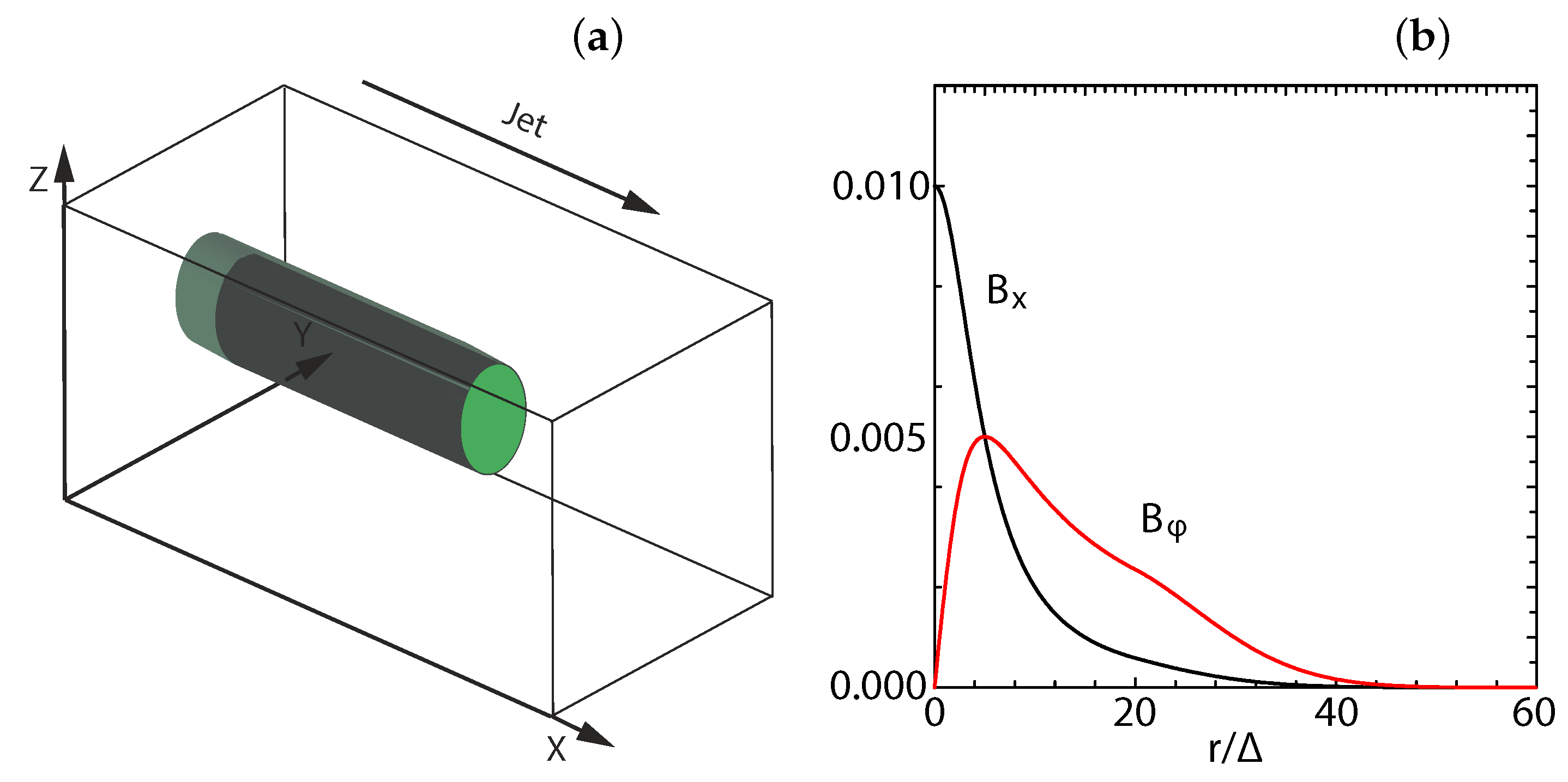
4.1. Helical Magnetic Field Structure

In the simulations of [61,62], cylindrical jets containing a helical magnetic field were injected into an ambient plasma (see Figure 6a). The structure of the helical magnetic field was implemented like that in the RMHD simulations performed by Mizuno et al. [68], where a force-free expression of the field at the jet orifice was used; that is, the magnetic field was not generated self-consistently, e.g., from simulations of jet formation by a rotating black hole. For the initial conditions, the force-free helical magnetic field was used as described in Equations (1) and (2) of Mizuno et al. (2014) [65].
The following form was used for the poloidal ( B x ) and the toroidal ( B ϕ ) components of the magnetic field determined in the laboratory frame:
B x = B 0 [ 1 + ( r / a ) 2 ] α , B ϕ = B 0 ( r / a ) [ 1 + ( r / a ) 2 ] α [ 1 + ( r / a ) 2 ] 2 α 1 2 α ( r / a ) 2 2 α 1 ,
where r is the radial coordinate in cylindrical geometry, B 0 parameterizes the magnetic field, a is the characteristic radius of the magnetic field (the toroidal field component has a maximum value at a, for a constant magnetic pitch), and α is the pitch profile parameter.
The expressions for describing the helical magnetic field used by [61,62] are written in Cartesian coordinates. Since α = 1 Equation (1) was reduced to Equation (2), the magnetic field takes the form:
B x = B 0 [ 1 + ( r / a ) 2 ] , B ϕ = ( r / a ) B 0 [ 1 + ( r / a ) 2 ] .
The toroidal component of the magnetic field was created by a current + J x ( y , z ) in the positive x-direction, and it is defined in Cartesian coordinates as:
B y ( y , z ) = ( ( z z jc ) / a ) B 0 [ 1 + ( r / a ) 2 ] , B z ( y , z ) = ( ( y y jc ) / a ) B 0 [ 1 + ( r / a ) 2 ] .
Here, the center of the jet is located at ( y jc , z jc ) and r = ( y y jc ) 2 + ( z z jc ) 2 . The chosen helicity is defined through Equation (3), which has a left-handed polarity with positive B 0 . At the jet orifice, the helical magnetic field is implemented without the motional electric fields. This corresponds to a toroidal magnetic field generated by jet particles moving along the + x -direction.
The poloidal ( B x : black) and the toroidal ( B ϕ : red) components of the helical magnetic field with a constant pitch ( α = 1 ) are shown in Figure 6b. The toroidal magnetic fields become zero at the center of the jet, as shown by red lines in Figure 6b. To date, simulations with a constant pitch ( α = 1 ) and with b = 200 have been performed using r jet = 20 , 40 , 80 , 120 Δ [61,62]. Here, b is the dumping factor of the magnetic fields outside the jet.
It should be noted that the structure of the jet formation region is more complicated than what is implemented in the PIC simulations at the present time (e.g., [69,70]). Furthermore, so far these global jet simulations have been performed with the simplest kind of jet structure with a top-hat shape (flat-density profile). A more realistic jet structure needs to be implemented in a future simulation study.

4.2. Helically Magnetized Global Jet Simulations with Larger Jet Radii

In this section, we explore how the jet evolution is affected by the helical magnetic field using a short system before performing more large-scale simulations. A schematic of the simulation injection setup is shown in Figure 6b [61,62]. The initial jet and ambient (electron and ion) plasma number density measured in the simulation frame is n jt = 8 and n am = 12 , respectively. This set of plasma parameters is used for obtaining the simulation results presented in [56,61,64].
In their simulations, the electron skin depth λ s = c / ω pe = 10.0 Δ , where c is the speed of light ( c = 1 ), ω pe = ( e 2 n am / ϵ 0 m e ) 1 / 2 is the electron plasma frequency, and the electron Debye length for the ambient electrons is λ D = 0.5 Δ . The jet–electron thermal velocity is v jt , th , e = 0.014 c in the jet reference frame. The electron thermal velocity in the ambient plasma is v am , th , e = 0.03 c , and ion thermal velocities are smaller by ( m i / m e ) 1 / 2 . Simulations were performed using an e ± plasma or an e p + (with m p / m e = 1836 ) plasma for the jet Lorentz factor of 15 and with the ambient plasma at rest ( v am = 0 ).
In these short system simulations, a numerical grid with ( L x , L y , L z ) = ( 645 Δ , 131 Δ , 131 Δ ) (simulation cell size: Δ = 1 ) is used, imposing periodic boundary conditions in transverse directions with a jet radius of r jet = 20 Δ [61]. In this review, all simulation parameters are maintained as described above except for the jet radius and the size of the simulation grid (which is adjusted based on the jet radius) [62]. Therefore, the jet radius is increased from the value r jet = 20 Δ up to several values: r jet = 40 Δ , 80 Δ , and 120 Δ , which corresponds to a numerical grid with ( L x , L y , L z ) = ( 645 Δ , 257 Δ , 257 Δ ) , ( 645 Δ , 509 Δ , 509 Δ ) , and ( 645 Δ , 761 Δ , 761 Δ ) , respectively. The cylindrical jet with jet radius r jet = 40 Δ , 80 Δ , and 120 Δ is injected into the middle of the yz plane ( ( y jc , z jc ) = ( 129 Δ , 129 Δ ) , ( 252 Δ , 252 Δ ) , ( 381 Δ , 381 Δ ) ) at x = 100 Δ . The largest jet radius ( r jet = 120 Δ ) is larger than that ( r jet = 100 Δ ) in [56], but the simulation length is much shorter ( L x = 2005 Δ ).
Other parameters used in their simulations include the initial magnetic field amplitude parameter B 0 = 0.1 c , where σ = B 2 / n e m e γ jt c 2 = 2.8 × 10 3 is used, and a = 0.25 r jet . The helical field structure inside the jet is defined by Equations (1) and (2). For the magnetic fields outside the jet, a damping function exp [ ( r r jet ) 2 / b ] ( r r jet ) is imposed on Equations (1) and (2) with the tapering parameter b = 200 Δ . The final profiles of the helical magnetic field components are similar to those obtained in the case where the jet radius is r jet = 20 Δ , with the only difference being that a = 0.25 · r jet , as it is shown in Figure 6b.
Figure 7 shows the y-component of the magnetic field ( B y ) for two values of the jet radius with r jet = 20 Δ and 80 Δ , respectively. In both cases, the initial helical magnetic field (left-handed; clockwise, viewed from the jet front) is enhanced and disrupted due to the plasma instabilities.
Thus, even when shorter simulation systems are used, growing instabilities are affected by the helical magnetic fields. The simple recollimation shock generated in the small jet radius is shown in Figure 7a,b. The currents generated by instabilities in the jets determine these complicated patterns of B y , as it is shown in Figure 7. Using a larger jet radius adds more modes of growing instabilities in the jets, which make the jet structure more complicated. In order to investigate the full development of instabilities in jets with helical magnetic fields, longer simulations are required.
To illustrate the production of acceleration of the particles in the jet, the Lorentz factor of the jet electrons was plotted for the two cases of plasma type used ( e p + and e ± , respectively) when the jet radius is r jet = 120 Δ , as it is shown in Figure 8. These observed patterns of the Lorentz factor coincide with the changing directions of the local magnetic fields in the y-direction, which are generated by kinetic instabilities like the Weibel instability, the kKHI, and the MI. The directions of the magnetic fields are indicated by the arrows (black spots) in the x z plane. (The arrows are better seen when the figure is magnified.) The directions of magnetic fields are determined by the generated instabilities. The structures at the edge of the jets are generated by the kKHI. Moreover, the plots of the Lorentz factor in the y z plane, which are not presented here, show the production of the MI at the circular edge of the jets.
Figure 9 shows the isosurface of the Lorentz factor of the jet electrons for a plasma that is composed of (a) e p + and (b) e ± . The 3D isosurface of the averaged jet electron Lorentz factor in a quadrant of the jet front ( 320 x / Δ 620 , 381 y , z / Δ 531 ) shows where jet electrons are accelerated (in reddish color) locally. The cross-sections and the surfaces of the jets show complicated patterns that are generated by mixed instabilities, where the fine lines represent the magnetic field lines.
For the jet radii larger than r jet = 80 Δ , the kKHI and the MI are generated at the jet surface, whereas inside the jet, the Weibel instability is generated together with a kink-like instability, particularly in the case of the e p + plasma. Answering the question on how the growth of kink-like instabilities depends on the helical magnetic fields requires further investigations using different parameters, including a, which determines the structure of the helical magnetic field in Equations (2) and (3). Furthermore, an imprint on the plasma behavior of different values of the pitch parameter α is also necessary for investigation using Equation (1).
Recently, Dieckmann et al. [57] investigated the expansion of a cloud of electrons and positrons with the temperature 400 keV that propagates at the mean speed 0.9c (c: speed of light) through an initially unmagnetized e p + plasma with PIC simulation. They found a mechanism that could collimate the pair cloud into a jet. The electrons and positrons of the cloud expanded rapidly due to their high temperature, which decreased the density of the cloud. A filamentation instability developed between the protons at rest and the moving positrons in the interval, where the latter were still dense. It is noted that it is difficult to distinguish the filament instability from the kKHI, which is shown in the simulation where the electron-positron jet was injected into an electron-positron ambient [56]. The instability expelled the protons from large areas, which were then filled with positrons. Magnetic fields grew only in those locations where protons and rapidly streaming positrons were present, which confined the magnetic field to a small spatial span. The effect of the filamentation instability and the resulting magnetic field were to push the protons away from the regions with no protons. The instability and the magnetic field followed the pushed protons and, hence, the filament grew in size. The largest filament grew along the reflecting boundary of their simulation, and the magnetic field that pushed the protons out became a stable magnetic piston. This filament is the largest one because the density of the cloud is largest where it is close to the boundary, and because it was aligned with the flow direction of the pair cloud. The large pool of directed flow energy was converted to magnetic field energy by the filament instability. Similar expansion of electron-positron jet plasmas was observed in the global jets without helical magnetic fields [56].
The filament was generated in a pair jet due to the separation by the generated magnetic field from the expelled and shocked ambient plasma. The front of the jet propagated with the speed 0.15c along the boundary and expanded laterally at a speed that amounted up to about 0.03c. The growth of the filament was limited by their simulation box size and by the limited cloud size; a decrease of the ram pressure would inevitably lead to a weakening of the filamentation instability and to a collapse of the jet. But it appears that, as long as the pair cloud has enough ram pressure, the filaments can grow to arbitrarily large sizes if the filamentation instability develops between a pair cloud and an electron-proton plasma, at least for plasma parameters similar to those used here. It should be noted that this simulation study shows the importance of kinetic processes of injected cylindrical plasma clouds using PIC simulation.

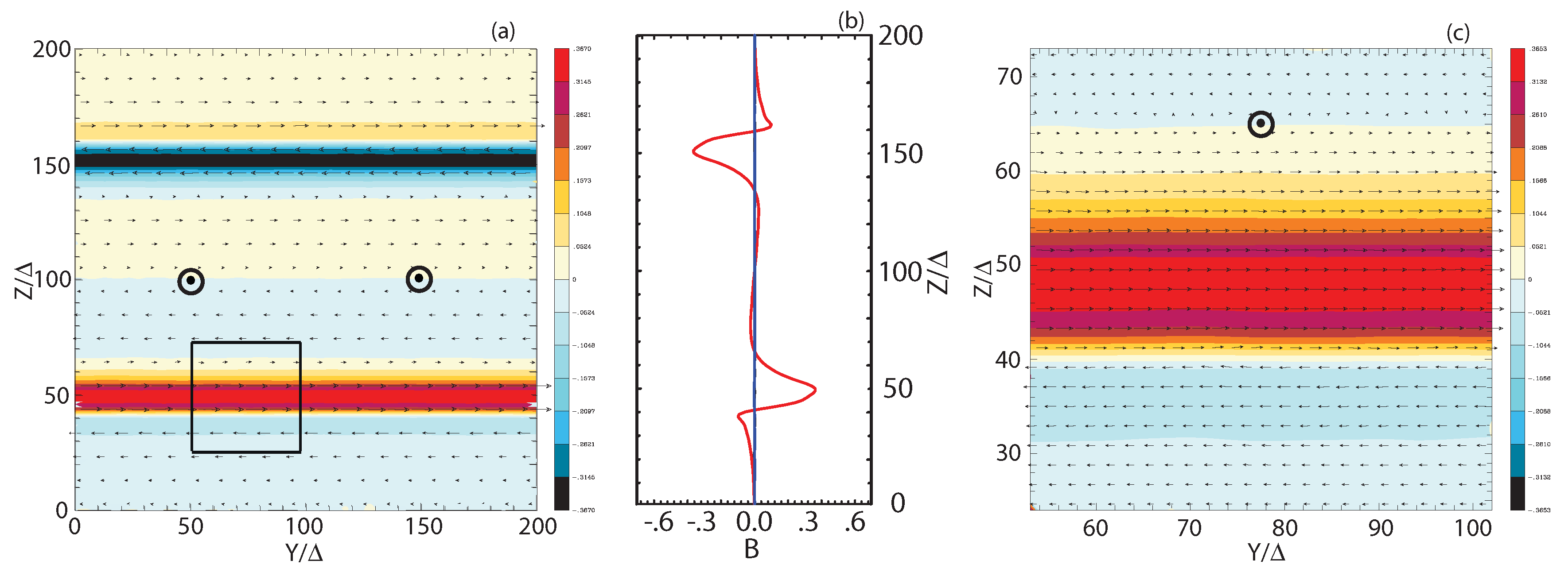
4.3. Reconnection in Jets with Helical Magnetic Fields

Reconnection is ubiquitous in solar and magnetosphere plasmas, and it is an important additional particle acceleration mechanism for AGN and GRB jets (e.g., [71]). Despite the extensive research on reconnection, most of all reconnection simulations have been performed with the Harris sheet [72]. where the unperturbed magnetic fields B are anti-parallel ( B = tanh ( x ) e y ). The release of energy stored in helical magnetic fields and particle acceleration during reconnection have been proposed as a mechanism for producing high-energy emissions and cosmic rays (e.g., [71,73]). It should be noted that the stored magnetic field energy in anti-parallel magnetic fields in the slab model is not consistent with the helical magnetic fields in the relativistic jets; therefore, a realistic argument on particle acceleration due to reconnection requires consideration of the helical magnetic field in the jets.
The importance of reconnection in jets has been proposed previously, but no kinetic simulation of global jets with helical magnetic fields has been performed before, with the exception of our own simulations [61,62].
Figure 10 shows the vectors of magnetic fields in the quadrant of the front part of the jets. Unfortunately, these vectors do not show the changes in direction which may reveal reconnection sites. In order to find the reconnection region, it is necessary to analyze the critical points (CPs). These CPs or magnetic nulls are the points where the magnitude of the magnetic field vector vanishes [74]. These points may be characterized by the behaviour of nearby magnetic field curves or surfaces. The set of curves or surfaces that end on CPs is of special interest because it defines the behaviour of the magnetic field in the neighborhood of CP.
The usual magnetic field configuration satisfies the hyperbolic conditions in which the vector field system has a nonzero real part of eigenvalues. The bifurcation (the topological change) represents the magnetic reconnection in the magnetic field. Thus, the particular sets of CPs, curves, and surfaces can be used to define a skeleton that uniquely characterizes the magnetic field [74]. In order to investigate the location of reconnection and its evolution, the method described by Cai, Nishikawa, and Lembege (2007) [74] needs to be employed in future work.

5. Discussion

In this paper, simulations of relativistic jets have been investigated extensively, starting from the study of the Weibel instability in slab mode, and continuing with simulations of instabilities in velocity-shears. Recently, a cylindrical geometry of the jets has been taken into account to be able to model the jet plasma more realistically.
The global jet simulations performed with large jet radii show the importance of a larger jet radius in PIC simulations for examining the macroscopic processes found in RMHD simulations. Due to the mixing of generated instabilities, the phase space plots of the jet electrons show little or no bunching in comparison to that when the jet radius is smaller, r jet = 20 Δ . Consequently, recollimation-like shocks occur, rather in the center of the jets. Moreover, the recollimation-like shock structure is dependent on the value of the parameter of the helical magnetic field geometry a. To better understand the production of such recollimation-like shocks, further investigations of PIC simulations performed with even larger radii of the jets are needed.
The Weibel instability is ubiquitous in plasma flows, particularly when the plasma is unmagnetized. However, as shown in one of the simulations with global e p + jets without helical magnetic fields, the Weibel instability is suppressed and the MI grows dominantly at the linear stage (see Figure 3a in Nishikawa et al. [56]). On the contrary, for e ± jets, the Weibel instability grows with the kKHI and the MI.
So far, the global jet simulations have been performed only for two values of the ion-to-electron -mass ratio, m i / m e = 1 and 1836. The simulation results obtained even when m p / m e = 1836 indicate that a small grid system is not appropriate for studying the kinetic plasma instabilities altogether in a realistic way. At this time, these two cases will provide us clearer differences between two different cases with the maximum mass ratio. In the simulations performed by Nishikawa et al. [61,62], only a weak magnetization factor was used. Simulations with stronger helical magnetic fields were performed by us, and preliminary results show that MI grows stronger with stronger magnetic fields. However, further investigation is necessary with larger systems.
These simulations show that the excitation of kinetic instabilities like the kKHI, the MI, and the Weibel instability with kink-like instability release the energy stored in the helical magnetic field. Consequently, jet and ambient electrons are accelerated and magnetic fields become turbulent. Furthermore, the accelerating electrons emit radiation, and the turbulent magnetic field induces the polarization of the emitted radiation.
MacDonald & Marscher [3] have developed a radiative transfer scheme that allows the Turbulent Extreme Multi-Zone (TEMZ) code to produce simulated images of the time-dependent linearly and circularly polarized intensity at different radio frequencies. Using the PIC simulation output data as input parameters in the TEMZ code, synthetic polarized emission maps were obtained. These maps highlight the linear and circular polarization expected within the above PIC models. This algorithm is currently being refined to account for slow-light interpolation through the global PIC simulations reviewed here.
Simulations of global jets with helical magnetic fields are promising in regard to providing new insights into jet evolution and associated phenomena. However, at the present time, the length of the system is too small, and a much longer system is required in order to investigate a nonlinear stage. Possibly even when using larger systems, such as a numerical grid with ( L x , L y , L z ) = ( 2005 Δ , 1005 Δ , 1005 Δ ) , the jet radius 100 Δ is not large enough to accommodate the microscopic processes, such as the gyro-motion of electrons and ions.
Therefore, these simulation results only provide some qualitative information which supplements those investigated by RMHD simulations. In the present simulations, jets were injected with a top-hat model. However, jets generated from black holes (either in AGN or in merging systems) have an opening angle and structured shapes. The helical magnetic fields used in the PIC simulations are not formed self-consistently as generated from rotating black holes like those performed in GRMHD simulations, and the initial setup with magnetic fields and the associated jet injection scheme need to be refined in future investigations. Furthermore, simulations of relativistic jets with large Lorentz factor particularly require the inclusion of radiation loss (e.g., [75]).
Since the power of supercomputers is growing rapidly, very large simulations of global jets could be performed, which will provide new insights on jet evolution, including reconnection and associated phenomena such as flares and high-energy particle generation.

Author Contributions

K.-I.N.: Perform simulations, analyze the data and prepare a manuscript; Y.M.: Understanding PIC simulation results based on RMHD simulations; J.L.G.: Contribute for comparing simulation results to observations; I.D.: Perform PIC simulations; A.M.: Perform simulations, critical reading and discussion on this research; J.N.: Contribute modifying the code for this research; O.K.; Modify the code for this simulation; M.P.: Overlook the simulation results; H.S.: Essential suggestions for this research; N.M.: Perform ray-tracing calculation for polarimetric images; D.H.H.: Useful discussions for this research.

Funding

This work is supported by NSF AST-0908010, AST-0908040, NASA-NNX09AD16G, NNX12AH06G, NNX13AP-21G, and NNX13AP14G grants. The work of J.N. and O.K. has been supported by Narodowe Centrum Nauki through research project DEC-2013/10/E/ST9/00662. Y.M. is supported by the ERC Synergy Grant “BlackHoleCam—Imaging the Event Horizon of Black Holes” (Grant No. 610058). M.P. acknowledges support through grant PO 1508/1-2 of the Deutsche Forschungsgemeinschaft. Simulations were performed using Pleiades and Endeavor facilities at NASA Advanced Supercomputing (NAS), and using Gordon and Comet at The San Diego Supercomputer Center (SDSC), and Stampede at The Texas Advanced Computing Center, which are supported by the NSF. This research was started during the program “Chirps, Mergers and Explosions: The Final Moments of Coalescing Compact Binaries” at the Kavli Institute for Theoretical Physics, which is supported by the National Science Foundation under grant No. PHY05-51164. The first velocity shear results using an electron−positron plasma were obtained during the Summer Aspen workshop “Astrophysical Mechanisms of Particle Acceleration and Escape from the Accelerators” held at the Aspen Center for Physics (1–15 September 2013).

Conflicts of Interest

The authors declare no conflict of interest.

References

  1. Hawley, J.; Fendt, C.; Hardcastle, M.; Nokhrima, E.; Tchekhovskoy, A. Disks and Jets. Galaxies 2015, 191. [Google Scholar] [CrossRef]
  2. Pe’er, A. Energetic and Broad Band Spectral Distribution of Emission from Astronomical Jets. Space Sci. Rev. 2014, 183, 371–403. [Google Scholar] [CrossRef]
  3. MacDonald, N.R.; Marscher, A.P. Faraday Conversion in Turbulent Blazar Jets. Astrophys. J. 2018, 862, 58. [Google Scholar] [CrossRef]
  4. Silva, L.O.; Fonseca, R.A.; Tonge, J.W.; Dawson, J.M.; Mori, W.B.; Medvedev, M.V. Interpenetrating Plasma Shells: Near-Equipartition Magnetic Field Generation and Nonthermal Particle Acceleration. Astrophys. J. Lett. 2003, 596, L121. [Google Scholar] [CrossRef]
  5. Nishikawa, K.I.; Hardee, P.; Richardson, G.; Preece, R.; Sol, H.; Fishman, G.J. Particle Acceleration in Relativistic Jets Due to Weibel Instability. Astrophys. J. 2003, 595, 555–563. [Google Scholar] [CrossRef] [Green Version]
  6. Frederiksen, J.T.; Hededal, C.B.; Haugbølle, T.; Nordlund, Å. Magnetic Field Generation in Collisionless Shocks: Pattern Growth and Transport. Astrophys. J. Lett. 2004, 608, L13. [Google Scholar] [CrossRef]
  7. Hededal, C.B.; Haugbølle, T.; Frederiksen, J.T.; Nordlund, Å. Non-Fermi Power-Law Acceleration in Astrophysical Plasma Shocks. Astrophys. J. Lett. 2004, 617, L107. [Google Scholar] [CrossRef]
  8. Hededal, C.B.; Nishikawa, K.I. The Influence of an Ambient Magnetic Field on Relativistic collisionless Plasma Shocks. Astrophys. J. Lett. 2005, 623, L89. [Google Scholar] [CrossRef]
  9. Nishikawa, K.I.; Hardee, P.; Richardson, G.; Preece, R.; Sol, H.; Fishman, G.J. Particle Acceleration and Magnetic Field Generation in Electron-Positron Relativistic Shocks. Astrophys. J. 2005, 622, 927. [Google Scholar] [CrossRef]
  10. Jaroschek, C.H.; Lesch, H.; Treumann, R.A. Ultrarelativistic Plasma Shell Collisions in γ-Ray Burst Sources: Dimensional Effects on the Final Steady State Magnetic Field. Astrophys. J. 2005, 618, 822. [Google Scholar] [CrossRef]
  11. Nishikawa, K.I.; Hardee, P.E.; Hededal, C.B.; Fishman, G.J. Acceleration Mechanics in Relativistic Shocks by the Weibel Instability. Astrophys. J. 2006, 642, 1267. [Google Scholar] [CrossRef]
  12. Nishikawa, K.I.; Hardee, P.; Hededal, C.; Richardson, G.; Preece, R.; Sol, H.; Fishman, G. Particle acceleration, magnetic field generation, and emission in relativistic shocks. Adv. Space Res. 2006, 38, 1316–1319. [Google Scholar] [CrossRef] [Green Version]
  13. Nishikawa, K.I.; Mizuno, Y.; Fishman, G.J.; Hardee, P. Particle Acceleration, Magnetic Field Generation, and Associated Emission in Collisionless Relativistic Jets. Int. J. Mod. Phys. D 2008, 17, 1761–1767. [Google Scholar] [CrossRef]
  14. Spitkovsky, A. On the Structure of Relativistic Collisionless Shocks in Electron-Ion Plasmas. Astrophys. J. Lett. 2008, 673, L39. [Google Scholar] [CrossRef]
  15. Spitkovsky, A. Particle Acceleration in Relativistic Collisionless Shocks: Fermi Process at Last? Astrophys. J. Lett. 2008, 682, L5. [Google Scholar] [CrossRef]
  16. Chang, P.; Spitkovsky, A.; Arons, J. Long-Term Evolution of Magnetic Turbulence in Relativistic Collisionless Shocks: Electron-Positron Plasmas. Astrophys. J. 2008, 674, 378. [Google Scholar] [CrossRef]
  17. Dieckmann, M.E.; Shukla, P.K.; Drury, L.O.C. The Formation of a Relativistic Partially Electromagnetic Planar Plasma Shock. Astrophys. J. 2008, 675, 586–595. [Google Scholar] [CrossRef] [Green Version]
  18. Nishikawa, K.I.; Niemiec, J.; Hardee, P.E.; Medvedev, M.; Sol, H.; Mizuno, Y.; Zhang, B.; Pohl, M.; Oka, M.; Hartmann, D.H. Weibel Instability and Associated Strong Fields in a Fully Three-Dimensional Simulation of a Relativistic Shock. Astrophys. J. Lett. 2009, 698, L10. [Google Scholar] [CrossRef]
  19. Martins, S.F.; Fonseca, R.A.; Silva, L.O.; Mori, W.B. Ion Dynamics and Acceleration in Relativistic Shocks. Astrophys. J. Lett. 2009, 695, L189. [Google Scholar] [CrossRef]
  20. Nishikawa, K.I.; Niemiec, J.; Medvedev, M.; Zhang, B.; Hardee, P.; Nordlund, A.; Frederiksen, J.; Mizuno, Y.; Sol, H.; Pohl, M.; et al. Radiation from relativistic shocks in turbulent magnetic fields. Adv. Space Res. 2011, 47, 1434–1440. [Google Scholar] [CrossRef] [Green Version]
  21. Choi, E.J.; Min, K.; Nishikawa, K.I.; Choi, C.R. A study of the early-stage evolution of relativistic electron-ion shock using three-dimensional particle-in-cell simulations. Phys. Plasmas 2014, 21, 072905. [Google Scholar] [CrossRef] [Green Version]
  22. Ardaneh, K.; Cai, D.; Nishikawa, K.I.; Lembége, B. Collisionless Weibel Shocks and Electron Acceleration in Gamma-Ray Bursts. Astrophys. J. 2015, 811, 57. [Google Scholar] [CrossRef]
  23. Ardaneh, K.; Cai, D.; Nishikawa, K.I. Collisionless Electron-ion Shocks in Relativistic Unmagnetized Jet-ambient Interactions: Non-thermal Electron Injection by Double Layer. Astrophys. J. 2016, 827, 124. [Google Scholar] [CrossRef]
  24. Grassi, A.; Grech, M.; Amiranoff, F.; Macchi, A.; Riconda, C. Radiation-pressure-driven ion Weibel instability and collisionless shocks. Phys. Rev. E 2017, 96, 033204. [Google Scholar] [CrossRef] [PubMed]
  25. Iwamoto, M.; Amano, T.; Hoshino, M.; Matsumoto, Y. Precursor Wave Emission Enhanced by Weibel Instability in Relativistic Shocks. Astrophys. J. 2018, 858, 93. [Google Scholar] [CrossRef] [Green Version]
  26. Takamoto, M.; Matsumoto, Y.; Kato, T.N. Magnetic Field Saturation of the Ion Weibel Instability in Interpenetrating Relativistic Plasmas. Astrophys. J. Lett. 2018, 860, L1. [Google Scholar] [CrossRef] [Green Version]
  27. Weibel, E. Spontaneously Growing Transverse Waves in a Plasma Due to an Anisotropic Velocity Distr. Phys. Rev. Lett. 1959, 2, 83–84. [Google Scholar] [CrossRef]
  28. Medvedev, M.V.; Loeb, A. Generation of Magnetic Fields in the Relativistic Shock of Gamma-Ray Burst Sources. Astrophys. J. 1999, 526, 697. [Google Scholar] [CrossRef]
  29. Medvedev, M.V.; Zakutnyaya, O.V. Magnetic Fields and Cosmic Rays in GRBs: A Self-Similar Collisionless Foreshock. Astrophys. J. 2009, 696, 2269. [Google Scholar] [CrossRef]
  30. Hoshino, M.; Shimada, N. Nonthermal Electrons at High Mach Number Shocks: Electron Shock Surfing Acceleration. Astrophys. J. 2002, 572, 880. [Google Scholar] [CrossRef]
  31. Amano, T.; Hoshino, M. Electron Injection at High Mach Number Quasi-perpendicular Shocks: Surfing and Drift Acceleration. Astrophys. J. 2007, 661, 190. [Google Scholar] [CrossRef]
  32. Amano, T.; Hoshino, M. Electron Shock Surfing Acceleration in Multidimensions: Two-Dimensional Particle-in-Cell Simulation of Collisionless Perpendicular Shock. Astrophys. J. 2009, 690, 244. [Google Scholar] [CrossRef]
  33. Sironi, L.; Spitkovsky, A.; Arons, J. The Maximum Energy of Accelerated Particles in Relativistic Collisionless Shocks. Astrophys. J. 2013, 771, 54. [Google Scholar]
  34. Guo, X.; Sironi, L.; Narayan, R. Non-thermal Electron Acceleration in Low Mach Number Collisionless Shocks. I. Particle Energy Spectra and Acceleration Mechanism. Astrophys. J. 2014, 794, 153. [Google Scholar] [CrossRef]
  35. Sironi, L.; Petropoulou, M.; Giannios, D. Relativistic jets shine through shocks or magnetic reconnection? Mon. Not. R. Astron. Soc. 2015, 450, 183–191. [Google Scholar] [CrossRef] [Green Version]
  36. Bret, A.; Alvaro, E.P. Robustness of the filamentation instability as shock mediator in arbitrarily oriented magnetic field. Phys. Plasmas 2011, 18, 080706. [Google Scholar] [CrossRef] [Green Version]
  37. Buneman, O. Tristan. In Computer Space Plasma Physics: Simulation Techniques and Software; TERRAPUB: Tokyo, Japan, 1993; Volume 1, pp. 67–100. [Google Scholar]
  38. Niemiec, J.; Pohl, M.; Stroman, T.; Nishikawa, K.I. Production of Magnetic Turbulence by Cosmic Rays Drifting Upstream of Supernova Remnant Shocks. Astrophys. J. 2008, 684, 1174. [Google Scholar] [CrossRef]
  39. Ramirez-Ruiz, E.; Nishikawa, K.I.; Hededal, C.B. e± Pair Loading and the Origin of the Upstream Magnetic Field in GRB Shocks. Astrophys. J. 2007, 671, 1877. [Google Scholar] [CrossRef]
  40. Mizuno, Y.; Lyubarsky, Y.; Nishikawa, K.I.; Hardee, P.E. Three-Dimensional Relativistic Magnetohydrodynamic Simulations of Current-Driven Instability. I. Instability of a Static Column. Astrophys. J. 2009, 700, 684. [Google Scholar] [CrossRef]
  41. Spitkovsky, A. Simulations of relativistic collisionless shocks: Shock structure and particle acceleration. In Astrophysical Sources of High Energy Particles and Radiation; Bulik, T., Rudak, B., Madejski, G., Eds.; American Institute of Physics Conference Series; Springer: Berlin, Germany, 2005; Volume 801, pp. 345–350. [Google Scholar]
  42. D’Angelo, N. Kelvin-Helmholtz Instability in a Fully Ionized Plasma in a Magnetic Field. Phys. Fluids 1965, 8, 1748–1750. [Google Scholar] [CrossRef]
  43. Gruzinov, A. GRB: Magnetic fields, cosmic rays, and emission from first principles? arXiv, 2008; arXiv:0803.1182. [Google Scholar]
  44. Mizuno, Y.; Hardee, P.; Nishikawa, K.I. Three-dimensional Relativistic Magnetohydrodynamic Simulations of Magnetized Spine-Sheath Relativistic Jets. Astrophys. J. 2007, 662, 835–850. [Google Scholar] [CrossRef]
  45. Perucho, M.; Lobanov, A.P. Kelvin-Helmholtz Modes Revealed by the Transversal Structure of the Jet in 0836+710. In Extragalactic Jets: Theory and Observation from Radio to Gamma Ray; Rector, T.A., De Young, D.S., Eds.; Astronomical Society of the Pacific Conference Series; Cornell University: San Francisco, CA, USA, 2008; Volume 386, pp. 381–387. [Google Scholar]
  46. Zhang, W.; MacFadyen, A.; Wang, P. Three-Dimensional Relativistic Magnetohydrodynamic Simulations of the Kelvin-Helmholtz Instability: Magnetic Field Amplification by a Turbulent Dynamo. Astrophys. J. Lett. 2009, 692, L40. [Google Scholar] [CrossRef]
  47. Alves, E.P.; Grismayer, T.; Martins, S.F.; FiÃza, F.; Fonseca, R.A.; Silva, L.O. Large-scale Magnetic Field Generation via the Kinetic Kelvin-Helmholtz Instability in Unmagnetized Scenarios. Astrophys. J. Lett. 2012, 746, L14. [Google Scholar] [CrossRef]
  48. Nishikawa, K.I.; Hardee, P.; Zhang, B.; DuÅ£an, I.; Medvedev, M.; Choi, E.J.; Min, K.W.; Niemiec, J.; Mizuno, Y.; Nordlund, A.; et al. Magnetic field generation in a jet-sheath plasma via the kinetic Kelvin-Helmholtz instability. Ann. Geophys. 2013, 31, 1535–1541. [Google Scholar] [CrossRef] [Green Version]
  49. Liang, E.; Boettcher, M.; Smith, I. Magnetic Field Generation and Particle Energization at Relativistic Shear Boundaries in Collisionless Electron-Positron Plasmas. Astrophys. J. Lett. 2013, 766, L19. [Google Scholar] [CrossRef]
  50. Grismayer, T.; Alves, E.P.; Fonseca, R.A.; Silva, L.O. dc-Magnetic-Field Generation in Unmagnetized Shear Flows. Phys. Rev. Lett. 2013, 111, 015005. [Google Scholar] [CrossRef]
  51. Grismayer, T.; Alves, E.P.; Fonseca, R.A.; Silva, L.O. Theory of multidimensional electron-scale instabilities in unmagnetized shear flows. Plasma Phys. Control. Fusion 2013, 55, 124031. [Google Scholar] [CrossRef]
  52. Liang, E.; Fu, W.; Boettcher, M.; Smith, I.; Roustazadeh, P. Relativistic Positron-Electron-Ion Shear Flows and Application to Gamma-Ray Bursts. Astrophys. J. Lett. 2013, 779, L27. [Google Scholar] [CrossRef]
  53. Alves, E.P.; Grismayer, T.; Fonseca, R.A.; Silva, L.O. Electron-scale shear instabilities: Magnetic field generation and particle acceleration in astrophysical jets. New J. Phys. 2014, 16, 035007. [Google Scholar] [CrossRef]
  54. Alves, E.P.; Grismayer, T.; Fonseca, R.A.; Silva, L.O. Transverse electron-scale instability in relativistic shear flows. Phys. Rev. E 2015, 92, 021101. [Google Scholar] [CrossRef] [PubMed]
  55. Nishikawa, K.I.; Hardee, P.E.; Duţan, I.; Niemiec, J.; Medvedev, M.; Mizuno, Y.; Meli, A.; Sol, H.; Zhang, B.; Pohl, M.; et al. Magnetic Field Generation in Core-sheath Jets via the Kinetic Kelvin-Helmholtz Instability. Astrophys. J. 2014, 793, 60. [Google Scholar] [CrossRef]
  56. Nishikawa, K.I.; Frederiksen, J.T.; Nordlund, Å.; Mizuno, Y.; Hardee, P.E.; Niemiec, J.; Gómez, J.L.; Pe’er, Å.; Dutan, I.; Meli, A.; et al. Evolution of Global Relativistic Jets: Collimations and Expansion with kKHI and the Weibel Instability. Astrophys. J. 2016, 820, 94. [Google Scholar] [CrossRef]
  57. Dieckmann, M.; Sarri, G.; Folini, D.; Walder, R.; Borghesi, M. Cocoon formation by a mildly relativistic pair jet in unmagnetized collisionless electron-proton plasma. Phys. Plasmas 2018, 25, 112903. [Google Scholar] [CrossRef]
  58. Nishikawa, K.I.; Hardee, P.; Dutan, I.; Zhang, B.; Meli, A.; Choi, E.J.; Min, K.; Niemiec, J.; Mizuno, Y.; Medvedev, M.; et al. Radiation from Particles Accelerated in Relativistic Jet Shocks and Shear-flows. arXiv, 2014; arXiv:1412.7064. [Google Scholar]
  59. Alves, E.P.; Zrake, J.; Fiuza, F. Efficient Nonthermal Particle Acceleration by the Kink Instability in Relativistic Jets. arXiv, 2018; arXiv:1810.05154. [Google Scholar] [CrossRef] [PubMed]
  60. Blandford, R.D.; Znajek, R.L. Electromagnetic extraction of energy from Kerr black holes. Mon. Not. R. Astron. Soc. 1977, 179, 433–456. [Google Scholar] [CrossRef] [Green Version]
  61. Nishikawa, K.I.; Mizuno, Y.; Niemiec, J.; Kobzar, O.; Pohl, M.; Gómez, J.L.; Dutan, I.; Pe’er, A.; Frederiksen, J.T.; Nordlund, Å.; et al. Microscopic Processes in Global Relativistic Jets Containing Helical Magnetic Fields. Galaxies 2016, 4, 38. [Google Scholar] [CrossRef]
  62. Nishikawa, K.I.; Mizuno, Y.; Gómez, J.L.; Dutan, I.; Meli, A.; White, C.; Niemiec, J.; Kobzar, O.; Pohl, M.; Pe’er, A.; et al. Microscopic Processes in Global Relativistic Jets Containing Helical Magnetic Fields: Dependence on Jet Radius. Galaxies 2017, 5, 58. [Google Scholar] [CrossRef]
  63. Tchekhovskoy, A. Launching of Active Galactic Nuclei Jets. In The Formation and Disruption of Black Hole Jets; Springer: Berlin, Germany, 2015; Volume 414, pp. 45–82. [Google Scholar]
  64. Dutan, I.; Nishikawa, K.I.; Mizuno, Y.; Niemiec, J.; Kobzar, O.; Pohl, M.; Gómez, J.L.; Pe’er, A.; Frederiksen, J.T.; Nordlund, Å.; et al. Particle-in-cell Simulations of Global Relativistic Jets with Helical Magnetic Fields. Proc. Int. Astron. Union 2016, 12, 199–202. [Google Scholar] [CrossRef] [Green Version]
  65. Mizuno, Y.; Hardee, P.E.; Nishikawa, K.I. Spatial Growth of the Current-driven Instability in Relativistic Jets. Astrophys. J. 2014, 784, 167. [Google Scholar] [CrossRef]
  66. Singh, C.B.; Mizuno, Y.; de Gouveia Dal Pino, E.M. Spatial Growth of Current-driven Instability in Relativistic Rotating Jets and the Search for Magnetic Reconnection. Astrophys. J. 2016, 824, 48. [Google Scholar] [CrossRef]
  67. Barniol Duran, R.; Tchekhovskoy, A.; Giannios, D. Simulations of AGN jets: Magnetic kink instability versus conical shocks. Mon. Not. R. Astron. Soc. 2017, 469, 4957–4978. [Google Scholar] [CrossRef]
  68. Mizuno, Y.; Gomez, J.L.; Nishikawa, K.I.; Meli, A.; Hardee, P.E.; Rezzolla, L. Recollimation Shocks in Magnetized Relativistic Jets. Astrophys. J. 2015, 809, 38. [Google Scholar] [CrossRef]
  69. Broderick, A.E.; Loeb, A. Imaging the Black Hole Silhouette of M87: Implications for Jet Formation and Black Hole Spin. Astrophys. J. 2009, 697, 1164. [Google Scholar] [CrossRef]
  70. Mościbrodzka, M.; Dexter, J.; Davelaar, J.; Falcke, H. Faraday rotation in GRMHD simulations of the jet launching zone of M87. Mon. Not. R. Astron. Soc. 2017, 468, 2214–2221. [Google Scholar] [CrossRef]
  71. Giannios, D.; Uzdensky, D.A.; Begelman, M.C. Fast TeV variability in blazars: Jets in a jet. Mon. Not. R. Astron. Soc. Lett. 2009, 395, L29–L33. [Google Scholar] [CrossRef]
  72. Harris, E.G. On a plasma sheath separating regions of oppositely directed magnetic field. Il Nuovo Cimento 1962, 23, 115–121. [Google Scholar] [CrossRef]
  73. Barniol Duran, R.; Leng, M.; Giannios, D. An anisotropic minijets model for the GRB prompt emission. Mon. Not. R. Astron. Soc. Lett. 2016, 455, L6–L10. [Google Scholar] [CrossRef]
  74. Cai, D.; Nishikawa, K.I.; Lembege, B. Visualization of Tangled Vector Field Topology and Global Bifurcation of Magnetospheric Dynamics. In Advanced Methods for Space Simulations; TERRAPUB: Tokyo, Japan, 2007; pp. 145–166. [Google Scholar]
  75. Cerutti, B.; Uzdensky, D.A.; Begelman, M.C. Extreme Particle Acceleration in Magnetic Reconnection Layers: Application to the Gamma-Ray Flares in the Crab Nebula. Astrophys. J. 2012, 746, 148. [Google Scholar] [CrossRef]
Figure 1. Averaged values of (a) the jet (red), the ambient (blue), and the total (black) electron density, and (b) electric (red) and magnetic (blue) field energy divided by the jet kinetic energy at t = 3250 ω p e 1 . Panel (c) shows the evolution of the total electron density in time intervals of δ t = 250 ω pe 1 . Diagonal lines indicate the motion of the jet front (blue: ≤c), the predicted contact discontinuity (CD) speed (green: ∼0.76c), and the trailing density jump (red: ∼0.56c). Adapted from Figure 1 in [18].
Galaxies 07 00029 g001
Figure 2. Structure of the flow, from the 3D simulation of an electron-positron shock with magnetization σ = 0 (top) or σ = 10 3 (bottom). Panels (b) and (d) show the particle density in the x y slice (with color scale stretched for clarity), whereas Panels (a) and (c) show the the magnetic energy fraction ϵ B in the x z and y z slices (with color scale stretched for clarity). Adapted from Figure 5 in [33].
Galaxies 07 00029 g002
Figure 3. Phase-space distribution of the jet (red) and the ambient (blue) electrons at t = 3250 ω p e 1 . About 18,600 electrons of both species are selected randomly. Adapted from Figure 2 in [18].
Galaxies 07 00029 g003
Figure 4. Magnetic field structure transverse to the flow direction for γ jt = 15 is shown in the y z plane (jet flows out of the page) at the center of the simulation box, x = 500 Δ for the e p + case. The small arrows show the magnetic field direction in the transverse plane (the arrow length is not scaled to the magnetic field strength). 1D cuts along the z axis of magnetic field components B x (black), B y (red), and B z (blue) are plotted at x = 500 Δ and y = 100 Δ for (b) the e p + case. Note that the magnetic field strength scales in panels (a) (±0.367) are different. An enlargement of the shear surface structure in the y z plane contained within the squares in the left panels is shown in the panels (c) to the right. Adapted from Figure 6 in Nishikawa et al. [55].
Galaxies 07 00029 g004
Figure 5. Isocontour plots of the J x magnitude with magnetic filed lines (one fifth of the jet size) for (a) an e p + and (b) an e e ± jet at simulation time t = 300 ω pe 1 . The 3D displays are clipped both along and perpendicular to the jet in order to view the interior. Adapted from Figure 4 in Nishikawa et al. [58].
Galaxies 07 00029 g005
Figure 6. Panel (a) shows a schematic simulation setup; a global jet setup. The jet is injected at x = 100 Δ with the jet radius r jet at the center of the y z plane (not scaled). Panel (b) shows the helical magnetic fields, B x ( black ) , B ϕ ( red ) with B 0 = 0.01 for the pitch profile α = 1.0 with damping functions outside the jet with b = 200.0 . The jet boundary is located at r jet = 20 Δ [61]. So far, simulations were performed with r jet = 20 , 40 , 80 , 120 Δ [62].
Galaxies 07 00029 g006
Figure 7. Isocontour plots of the azimuthal component of magnetic field B y intensity at the center of the jets for e p + (a,c) e ± (b,d) jets; with r jet = 20 Δ (a,b) r jet = 80 Δ (c,d) at time t = 500 ω pe 1 . The disruption of helical magnetic fields are caused by instabilities and/or reconnection. The max/min numbers of panels are (a) ±2.645, (b) ±2.427, (c) ±3.915, (d) ±1.848. Adapted from Figure 1 in Nishikawa et al. [62].
Galaxies 07 00029 g007
Figure 8. Panels (a,b) show the 2D plot of the Lorentz factor of jet electrons for e p + (a) and e ± (b) jet with r jet = 120 Δ at time t = 500 ω pe 1 . The arrows (black spots) show the magnetic fields in the x z plane. Adapted from Figure 3 in Nishikawa et al. [62].
Galaxies 07 00029 g008
Figure 9. Panels show 3D isosurface plots of the Lorentz factor of the jet electrons for e p + (a) and e ± (b) jet with r jet = 120 Δ at time t = 500 ω pe 1 . The lines show the magnetic field stream lines in the quadrant of the front part of the jets. The color scales for contour (upper left): red 20.0; orange 13.67; right blue 7.33 . blue 1. The color scales of streaming lines (a) (5.92, 3.52, 0.174, 1.29 , 3.70 ) × 10 1 ; (b) (3.96, 2.21, 0.453 , 1.30 , 3.05 ) × 10 1 . Adapted from Figure 4 in Nishikawa et al. [62].
Galaxies 07 00029 g009
Figure 10. Panels show 3D vector plots of the magnetic fields for the (a) e p + and (b) e ± jets with r jet = 120 Δ at time t = 500 ω pe 1 . The colors show the strength of the magnetic fields in the quadrant of the front part of the jets.
Galaxies 07 00029 g010

