Abstract
According to the standard cold dark matter (CDM) cosmology, the structure of dark halos including those of galaxy clusters reflects their mass accretion history. Older clusters tend to be more concentrated than younger clusters. Their structure, represented by the characteristic radius and mass of the Navarro–Frenk–White (NFW) density profile, is related to their formation time. In this study, we showed that , , and the X-ray temperature of the intracluster medium (ICM), , form a thin plane in the space of . This tight correlation indicates that the ICM temperature is also determined by the formation time of individual clusters. Numerical simulations showed that clusters move along the fundamental plane as they evolve. The plane and the cluster evolution within the plane could be explained by a similarity solution of structure formation of the universe. The angle of the plane shows that clusters have not achieved “virial equilibrium” in the sense that mass/size growth and pressure at the boundaries cannot be ignored. The distribution of clusters on the plane was related to the intrinsic scatter in the halo concentration–mass relation, which originated from the variety of cluster ages. The well-known mass–temperature relation of clusters () can be explained by the fundamental plane and the mass dependence of the halo concentration without the assumption of virial equilibrium. The fundamental plane could also be used for calibration of cluster masses.
1. Introduction
Clusters of galaxies are the most massive objects in the Universe. Since the fraction of baryons in clusters is not much different from the cosmic mean value, dark matter accounts for most of the mass of clusters (∼84%) [1,2]. Thus, the structure of the clusters is mainly determined by the halos of dark matter, or the dark halos. Cold dark matter (CDM) cosmology predicts that more massive halos form later. Thus, clusters form after galaxies do. However, the definition of the formation is not obvious, because halos are continuously growing through mergers and accretion from their environments. A current trend may be associating the formation time with the internal structure of dark halos.
The density distribution of dark halos is well-represented by the Navarro–Frenk–White (NFW) density profile [3,4]:
where r is the clustercentric radius, is the characteristic radius, and is the critical density of the universe. The normalization of the profile is given by . The characteristic mass is defined as the mass inside and the characteristic density is written as . The mass profile of the NFW profile is written as
Another commonly defined characteristic radius of clusters is that based on the critical density ; it is represented by , which is the radius of a sphere of mean interior density , where is the constant. The mass within is written as
The radius when or is often called the “virial radius”. Since it is generally difficult to observationally study cluster properties out to , is also used as a representative value. The ratio
is called the halo concentration parameter and for and 500 for clusters.
Navarro et al. [4] pointed out that the characteristic parameters of the NFW profile (e.g., and ) reflect the density of the background universe when the halo was formed. This means that, since older halos formed when the density of the universe was higher, they tend to have larger characteristic densities and become more concentrated with larger . This issue has been addressed in many studies, especially by N-body simulations [4,5,6,7,8,9,10,11,12,13,14,15,16,17,18]. These studies have indicated that the halo structure is determined by their mass-growth history. The inner region ()1 of current halos develops in the early “fast-rate growth” phase when the halos grow rapidly through matter accumulation. Their outer region () is formed in the subsequent “slow-rate growth” phase in which halos grow slowly through moderate matter accumulation. During this phase, the inner region is almost preserved. Thus, halos form “inside-out”. The formation time of a halo can be defined as the transition time from the fast-rate growth phase to the slow-rate growth phase. This shift of the growth phase is largely associated with the decrease in the average density of the universe in the CDM cosmology. There are a few specific definitions of the formation time that well represent the transition time. One is the time at which the mass of the main progenitor was equal to the characteristic mass of the halo at its observed redshift [14,15]. The formation redshift () corresponding to the formation time should be larger than , or . For a given , clusters with a larger have a larger and .
Moreover, numerical simulations have shown that clusters are dynamically evolving systems and such evidence is often found in their outskirts. In fact, the ambient material is continuously falling toward clusters, which creates “surfaces” around clusters. For example, the outskirt profiles of dark matter halos can become extremely steep over a narrow range of radius (“splashback radius”). This features in the density profiles are caused by splashback of collisionless dark matter on its first apocentric passage after accretion [19,20]. Accretion of collisional gas toward clusters also creates discontinuities in the form of shock fronts in their outskirts [21,22]. These discontinuities mean that clusters are neither isolated nor in an equilibrium state.
In this review, we first introduce the fundamental plane we discovered, and its implications for structure formation of the universe. In particular, we show that clusters in general have not achieved virial equilibrium in contrast with conventional views. Then, using the fundamental plane, we discuss that a scaling relation (mass-temperature relation) can be explained without assuming virial equilibrium. We also show that the fundamental plane can be used for mass calibration. We assume a spatially-flat CDM cosmology with , , and the Hubble constant of km s Mpc.
2. Fundamental Plane
The hot intracluster medium (ICM) is distributed in the potential well of dark halos. Since the X-ray emission from the ICM is proportional to the square of the density, it mainly comes from the central region of the cluster where the density is high. Thus, the observed X-ray temperature represents that of the central region and should reflect the gravitational potential there. Since the potential is determined by and , we can expect some relation among , , and .
Based on this motivation, Fujita et al. [23] analyzed 20 massive clusters in the Cluster Lensing And Supernova survey with Hubble (CLASH) observational sample [24,25]. For these clusters, and had been obtained from the joint analysis [26] of strong lensing observations with 16-band Hubble Space Telescope observations [27] and weak-lensing observations mainly with Suprime-Cam on the Subaru Telescope [28]. The X-ray temperature had been obtained with Chandra [24,29]. Temperatures are estimated for a cylindrical volume defined by the projected radii –500 kpc to avoid the influence of cool cores. Figure 1a shows the data distribution in the space. As can be seen, the data are distributed on a plane. The plane is described by , with , , and . Figure 1b shows the cross-section of the plane; the dispersion of the data around the plane is very small and is only dex (all uncertainties are quoted at the confidence level unless otherwise mentioned). In Figure 1c, error bars for individual clusters are shown. In the vertical direction (), we show the temperature errors of individual clusters. In the horizontal direction, the errors of and are strongly correlated, and we display them as a single bar. This means that we draw a bar connecting (, ) and (, ) for each cluster, where the superscripts u and l are the upper and the lower limits, respectively. We note that, when we calculate the plane parameters, we properly account for the correlation for each cluster using the joint posterior probability distribution of the NFW parameters (mass and concentration) [23]. Thus, the actual error is not represented by a single bar in a precise sense. Figure 2 shows the direction of the plane normal in the space [23]. The contours are drawn considering the errors and show that the direction is inconsistent with the prediction of a simplified dimensional analysis or . We note that it is meaningless to discuss cluster distribution in the space of , where , , and are their current values. Although the clusters form a plane in that space, it is just the obvious relation of regardless of (Section 5.3 in [23]).
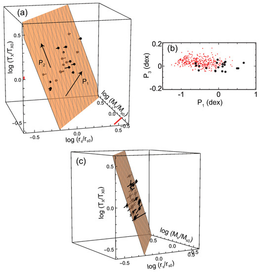
Figure 1.
(a) Black dots (pin heads) are the CLASH data in the space of , , , where kpc, , and keV are the sample geometric averages (log means) of , , and , respectively. The orange plane is the best fit of the data. The orange plane is translucent, and the grayish points are located below the plane. The lengths of the pins show the distance to the plane. The red bars show typical errors of the data. The arrow shows the direction to which the data distribution is most extended, and the arrow is perpendicular to on the plane. (b) The cross-section of the plane in (a). The large black dots are the CLASH data, and the small red dots are the MUSIC results shown in Figure 3. The latter is projected on the – plane determined for the former. The direction is the plane normal. Note that the scales of the vertical and horizontal axes are different. (c) The same as (a) but error bars for individual clusters are included. The viewing angle is changed so that the relation between the error bars and the plane is easily seen (Figure is reconstructed from Figure 1 of [23]).
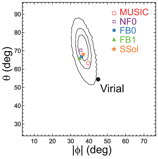
Figure 2.
The angle of the plane normal in the space of ; is the angle between and the axis, and is the azimuthal angle around the axis, measured anti-clockwise from the axis. The contours are for the CLASH observational data showing the 68% (1), 90% and 99% confidence levels from inside to outside. The large black dot (Virial) is the prediction of the simplified dimensional analysis or and is rejected at the >99% level. The directions of the plane normals estimated for the simulation samples MUSIC, NF0, FB0, and FB1 are shown by the open red circle, the open purple square, the filled blue square, and the filled green triangle, respectively. The prediction of the similarity solution (Equation (9) for ) is shown by the orange star (SSol) (Figure is reconstructed from Figure 2 of [23]).
The “fundamental plane” 2 has been reproduced by numerical simulations. Figure 3 shows the results of MUSIC N-body/hydrodynamical simulations (see details in [23,25]). These simulations do not include radiative cooling or non-gravitational feedback by active galactic nuclei (AGNs) and supernovae (SNe). The mass resolutions for the dark-matter particles that for the gas particles are and , respectively, where the Hubble constant is written as km s Mpc and . The gravitational softening is set to be 6 kpc for the both gas and dark-matter particles in high-resolution regions. We chose all 402 clusters at with regardless of dynamical state. In this analysis, we included the core because these simulations are non-radiative and thus do not present cool-core features. The absolute position of the plane is very close to that of the CLASH observational data (Figure 1b). Figure 2 shows that the plane angle for the MUSIC sample is consistent with the CLASH data at the 90% confidence level.
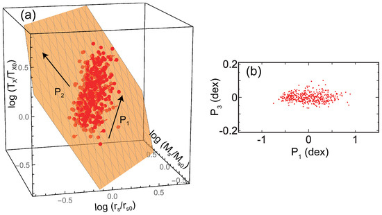
Figure 3.
(a) Red dots (pin heads) are the results of the adiabatic MUSIC simulations (). The axes are normalized by the average parameters of the sample ( kpc, , and keV). The orange plane is the best fit of the data. The arrow shows the direction to which the data distribution is most extended, and the arrow is perpendicular to on the plane. (b) The cross-section of the plane in (a). The direction is the plane normal (Figure is reconstructed from Figure 3 of [23]).
Figure 4 presents the results of other numerical simulations including phenomena such as heating by AGNs and SNe in addition to radiative cooling (see details in [23,37]). Sample FB0 (blue dots) consists of the clusters at , while sample FB1 (green dots) refers to the runs at . These runs simulate 29 Lagrangian regions around massive clusters with – at . The mass resolution for the dark-matter particles and the initial gas particles are and , respectively. In high-resolution regions the gravitational softening is set to be kpc [38]. For the gas particles, this is always in comoving units, while for the DM particles it changes to physical units from to . For these samples, the temperature is estimated for –500 kpc, and thus the influence of cool cores is removed. Both groups of dots are located on almost the same fundamental plane, and the plane angles for the two samples are almost the same (Figure 2). This means that clusters evolve along the unique plane in the direction of in Figure 4a. The plane angles for FB0 and FB1 are not much different from those for the CLASH data and the MUSIC adiabatic simulations (Figure 2). In Figure 2, NF0 is the result of a simulation that is the same as FB0 but not including radiative cooling and feedback. Since their angles are almost the same, this indicates that radiative cooling and feedback do not much affect the fundamental plane. This is because we are discussing cluster properties on a scale of kpc, and the influences of cool cores, where radiative cooling and feedback are especially important, are ignorable.
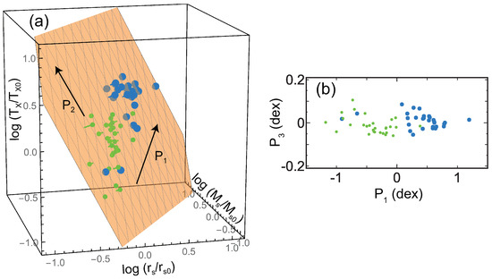
Figure 4.
(a) The results of simulations including radiative cooling and feedback. The blue (FB0) and the green dots (FB1) are the results for and 1, respectively. The axes are normalized by the average parameters of the combined sample ( kpc, , and keV). The orange plane is the best fit of the data. The arrow shows the direction to which the data distribution is most extended, and the arrow is perpendicular to on the plane. (b) The cross-section of the plane in (a). The direction is the plane normal (Figure is reconstructed from Figure 4 of [23]).
3. Origin of the Fundamental Plane and Cluster Growth
Fujita et al. [23] explained the origin of the fundamental plane using an analytic similarity solution developed by Bertschinger [39] (see also [40]). This solution treats spherical collapse of an overdense region in the Einstein–de Sitter universe () and subsequent matter accretion onto the collapsed object. In the solution, matter profiles are represented by non-dimensional radius, , density , pressure , and mass . The solution has a constant called the “entropy constant”.
where is the adiabatic index. The non-dimensional parameters are related to dimensional density , pressure p, and mass m:
where is the maximum radius that a mass shell reaches (the turnaround radius), is the density of the background universe, and t is the cosmological time. The non-dimensional radius is given by . We note that the similarity solution describes the matter profile in the region where the matter is later accreted (say, ). The solution was originally developed for objects totally composed of baryons, thus , p, and m are for the gas. However, the non-dimensional profiles (D, p, and M) are not much changed, even if objects are mostly composed of dark matter [39]. Thus, the profiles , p, and m can be regarded as the values for the gas as long as we do not discuss the normalizations. Although the solution is constructed for the Einstein–de Sitter universe, it well-reproduces the structure of objects except for the outermost region even for a CDM universe, because the inner region was established when the background density of the universe was large [39]. From Equations (5) and (6), we obtain , where and is time-independent. Here, and are the turnaround radius (the maximum radius before the collapse) and the turnaround time (the time when the radius reaches turnaround radius) of the overdense region, respectively. The evolution of the overdense region is described by the conventional spherical collapse model. Thus, it should follow the spectrum of initial density perturbations of the universe and the mass of the overdense region has scaling relations of
where n, the spectral index, is of the initial density perturbations [41] and is expected around the mass scales of clusters [42,43]. Here, we emphasize that Equation (7) is applied to the overdense region, and not to the entire cluster, because we separately treat the initial collapse of the overdense region and the subsequent matter accretion. Thus, we obtain . Assuming that , and at , it is written as
The radius 3 and the mass of the overdense region can be connected to the characteristic radius and mass of the NFW profile. This is because the evolution of both overdense region in the similarity solution and the inner region of the NFW profile () is related to the background universe, and they evolve in a similar way. In fact, the evolution of the former is described by the conventional spherical collapse of an overdense region [39], and thus the typical density is proportional to that of the background universe at the collapse. The same applies to the latter because the characteristic density is always ∼900 times as large as that of the background universe at the formation redshift [15]. Thus, we can assume that and , and that the collapse time of the overdense region (∼2 ; see, e.g., [44], Section 19) corresponds to the formation redshift . In summary, the similarity solution has scales such as and . Since and are proportional to and , respectively, the solution has scales of and . These scales represent the border between the initially-collapsed overdense region and the later-accreted region, although the actual transition is gradual. This also means that the initial collapse and the later accretion correspond to the fast-rate growth phase and the slow-rate growth phase, respectively. Finally, from Equation (8), we obtain
or . Equation (9) forms a plane in the space. The direction of the normal when is shown in Figure 2 as “SSol”, and it is consistent with the CLASH observations and the results of numerical simulations. Note that this relation (Equation (9)) is independent of redshift z at least (Figure 4), because and are physical values that have already reflected the high density of the background universe in the past.
The similarity solution indicates that clusters are not in virial equilibrium, because clusters are growing through matter accretion from their outer environments [39,40]. That is one reason clusters follow Equation (9) instead of , which could be realized if clusters are in virial equilibrium at their formation. The condition of the virial “equilibrium” is represented by , where K is the kinetic and/or thermal energy and W is the gravitational energy. However, according to the virial “theorem”, which is a higher-level concept of the virial “equilibrium”, additional terms are required when clusters are growing [39,40]. One is the term representing the increase of mass and size of clusters and another is the boundary term originating from the flux of inertia through the boundary and the pressure at the boundary. The boundary corresponds to the splashback radius for dark matter and the shock front for gas (see Section 1). Note that the similarity solution shows that clusters are almost in hydrostatic equilibrium in the sense that gas motion is negligible within clusters even if they are not in virial equilibrium [39]. The relation between matter accretion and the cluster structure has also been numerically studied (e.g., Reference [18]).
Figure 5 shows the projection of the fundamental plane shown in Figure 3 on the – plane. The solid arrow is parallel to the line of along which the distribution of the MUSIC clusters (red points) is elongated. This direction is also close to that of cluster evolution () in Figure 4 projected on the – plane [23]. Since we assumed that and , the line corresponds to the first relation of Equation (7) when . Considering the derivation of the relations in Equation (7) (see [41]), this indicates that the evolution of clusters on the fundamental plane reflects the spectrum of the initial density perturbations of the universe and follows [41]. Figure 5a also shows that the characteristic density decreases as a cluster moves in the direction of the solid arrow. While the formation redshift is formally related to the collapse time of the overdense region, in reality, it is often related to the time of major cluster mergers. That is, the formation redshift is reset when the cluster experiences a major merger, and estimated from for a given cluster at often corresponds to the time when the cluster underwent its last major merger. In fact, numerical simulations have shown that an individual cluster intermittently moves in the direction of the solid arrow in Figure 5 every time it undergoes mergers [23]. While the cluster temporarily deviates the general motion in the middle of a major merger, the deviation is confined in the fundamental plane and thus mergers do not much affect the thinness of the plane [23]. In other words, the effect of major cluster mergers introduces some random history that could be different for clusters of the same mass, but since the mergers move cluster properties within the limits of the plane, the scatter of the plane does not increase very much.
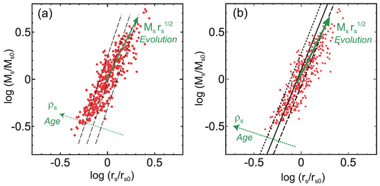
Figure 5.
Projection of the fundamental plane on the – plane shown in Figure 3. (a) The red points show the MUSIC clusters () and and are the same as those in Figure 3. The solid arrow shows the direction of cluster evolution () and increases in this direction. The cluster age and increase in the direction of the dotted arrow. Each dashed line satisfies = const or clusters on a particular line have the same formation redshift . (b) The same as (a) but – relation transformed from – relation is drawn (black solid line). Black dotted and dashed lines correspond to the dispersion of – relation (±0.1 dex) shown by numerical simulations (Figures are reconstructed from Figure 5a of [23] and Figure 2 of [47]).
We would like to point out that in Figure 5 simulated clusters are not tightly distributed along the line of (solid arrow), and there is a scatter about the line. This reflects the fact that the density perturbations of the universe are described by a Gaussian random field (see, e.g., [45]). Thus, while the variance of the perturbation field is a decreasing function of mass scale M, the amplitudes of the perturbations that collapse into objects with a given mass M are not always . Owing to this, for example, and are not perfectly in one-to-one correspondence, and has some range for a given , which produces the band-like distribution of clusters in Figure 5 and on the fundamental plane (Figure 1a, Figure 3a and Figure 4a). In other words, clusters form a two-parameter family. Thus, a correlation between two physical quantities is generally represented by a band rather than a line unless some special combination of quantities is chosen. In that sense, it is natural that the relation between and has a large dispersion [5,14,15,25,46], which will be discussed in Section 4. On the fundamental plane, different clusters move along nearly parallel but different tracks each of which approximately follows the relation of [23]. While the temperature of each cluster is affected by its formation time, it also depends on the track the cluster chooses.
4. Mass–Temperature Relation and the Concentration Parameter
The fundamental plane can be used to relate the cluster structure to the temperature. As an application, we discuss the mass–temperature relation in this section. It is well-known that the mass of clusters and the X-ray temperature has a relation of . This relation is obtained by both observations and numerical simulations [48,49,50,51]. Conventionally, this relation has been explained based on the following three assumptions: (i) the typical density of a cluster is (not ); (ii) clusters are well-relaxed or virialized, and they are almost isothermal within ; and (iii) the X-ray temperature is determined on a scale of (not ). Here, we consider cluster temperature outside cool cores.
The density is represented by , where is the Hubble parameter at redshift z normalized by the current value . Equation (3) is associated with Assumption (i). From Assumptions (ii) and (iii), we obtain . Eliminating by using the relation , the mass–temperature relation is obtained:
which well reproduces the results of observations and simulations [48,52,53]. However, the assumptions are clearly inconsistent with the inside-out scenario of cluster formation and the fundamental plane. For example, the inside-out scenario indicates that clusters are not well relaxed and keep the memory of their formation in their structure. The angle of the fundamental plane shows that clusters are not virialized, as discussed in Section 3. The NFW profile (Equation (1)) is not an isothermal profile (). These are inconsistent with Assumption (ii). Moreover, the tight correlation of the fundamental plane shows that is determined by and , which contradicts Assumption (iii).
In [47], Fujita et al. showed that the relation in Equation (10) can be derived using the fundamental plane and the halo concentration–mass (–) relation. The fundamental plane relation in Equation (9) is rewritten as
where corresponds to a representative point on the fundamental plane, and we adopt kpc, , and keV based on the results of the MUSIC simulations [23,25]. Based on the inside-out scenario, there are analytical forms of the concentration parameter represented as a function of and z. One example is
for that was obtained by Duffy et al. [46] (see also [25,43,54,55,56]). From Equation (3), we obtain
Equations (4), (12) and (13) indicate that is a function of for a given z. Moreover, Equation (2) suggests that is also a function of :
Thus, using Equation (11), can be represented as a function of for a given z. Figure 6a shows the results for using a general formula of developed by Correa et al. [15] instead of Equation (12). The slope is for and for (). The slope is close to but slightly smaller than . However, the derivation of the fundamental plane in Section 3 might be too simplified, and there might be some minor uncertainties on n [47]. In fact, if we take , the slope becomes for and for . Note that, even if we assume , the direction of the fundamental plane (Equation (9)) is consistent with observations and simulations [47]4. Thus, the relation of can be reproduced without the virial assumption or . Note that Figure 6 indicates that the red lines () are slightly below the black lines (). This may cause some bias about the slope index if clusters with various redshifts are plotted at the same time. For example, if higher-redshift clusters () tend to have smaller masses and lower temperatures than lower-redshift clusters (), the slope is slightly steepened (larger ). We note that Voit [57] (see also [58]) already addressed this issue. He considered accretion history of clusters and the effects of cluster surfaces as we do. While we focused on the inner structure of clusters, he studied the evolution of global properties of clusters. He concluded that the approximate agreement between the – relation derived via the traditional collapse model (Equation (10)) and those of simulations and observations is largely coincidental. Although our approach is different, our results support the conclusion.
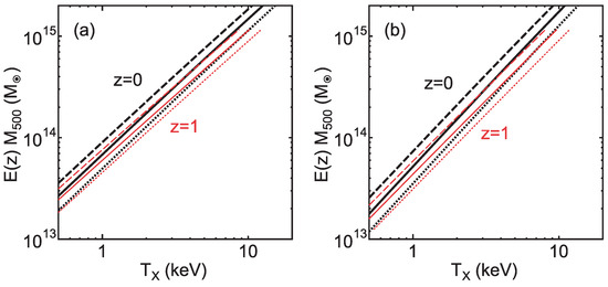
Figure 6.
– relation for derived from the fundamental plane and the – relation (solid lines): (a) ; and (b) . The thick black lines and the thin red lines represent and 1, respectively. Dotted and dashed-lines correspond to the dispersion of the – relation (±0.1 dex) shown by numerical simulations (Figures are reconstructed from Figure 1 of [47]).
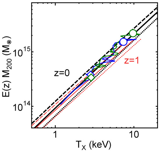
The relation of – or the function can be converted into the relation between and using Equations (3), (4), and (14), and the result is shown by the solid black line in Figure 5b. The black dotted and dashed lines correspond to the dispersion of – relation indicated by numerical simulations. The three black lines in Figure 5b are almost parallel to the lines of const or the three black dashed lines in Figure 5a. This means that the dispersion of – relation is almost the same as that of or the dispersion of cluster formation time . Figure 5b also indicates that the minor axis of the cluster distribution (red points) corresponds to the dispersion of the – relation. The dispersion of the – relation is also associated with that of the – relation, which is indicated by the black dotted and dashed lines in Figure 6. In Figure 7, we present the evolution of simulated clusters along the – relation. As expected, the clusters move along the bands enclosed by the dotted and dashed lines. The clusters frequently move in the horizontal direction, which corresponds to temporal temperature increase during cluster mergers. However, even during the mergers, the clusters are located within the bands, which means that the – relation is not much affected by mergers.
5. Cluster Mass Calibration
The thinness and solidity of the fundamental plane inspires applications in cosmology. Here, we show that the plane can be used to calibrate cluster mass [47]. Precise estimation of cluster mass is important. For example, when cosmological parameters are derived from cluster number counts, scaling relations among observables are used and they are affected by the calibration of cluster mass [59].
Figure 8a shows the cross sections of the fundamental plane. The red open circles are the clusters of the CLASH sample [24], for which and are derived through gravitational lensing. The black dots are those of an X-ray sample [60], for which and are derived through X-ray observations assuming that the ICM is in hydrostatic equilibrium. We discuss the fundamental plane formed by the CLASH sample (CFP) and the one formed by the X-ray sample (XFP) separately. Fixing the direction of the plane normals at the one shown by SSol in Figure 2, the distance between the two fundamental planes is estimated to be dex in the space of . Thus, the position of the fundamental planes are consistent with each other. However, the XFP seems to be located slightly above the CFP in Figure 8a. The shift may be caused by a possible systematic difference of observed or between CFP and XFP because they are obtained through different methods (gravitational lensing and X-ray observations). The plane shift in the direction of or can be estimated from . Then, assuming the NFW profile (Equation (1) or (2)), the shift in the direction of can be derived [47].
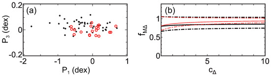
Figure 8.
(a) Cross sections of the fundamental plane. Red open circles are the CLASH clusters (CFP) and black dots are the X-ray clusters (XFP). (b) Relation between and concentration parameter . Solid lines are the fiducial relations and the dash-dotted lines show uncertainties. The difference of black and red lines come from the different assumptions of the plane shift (see [47]) (Figures are reconstructed from Figures 5 and 6 of [47]).
Figure 8b shows the systematic difference of , which is defined by , where is the mass of a cluster on the XFP, and is the mass of the same cluster on the CFP. While the ratio depends on the concentration parameter , the dependence is weak. Figure 8b shows that , which means that the cluster mass estimated through X-ray observations assuming hydrostatic equilibrium (hydrostatic mass) is ∼15% smaller than that estimated through gravitational lensing. Since the error is rather large, the current dataset may not be accurate enough for the calibration purpose. However, the error could be reduced by using larger and more accurate datasets in the future. Assuming that gravitational lensing mass is solid, the value of is consistent with the results of numerical simulations showing that hydrostatic mass tends to be smaller than the true mass [61,62,63,64].
6. Sparsity
Finally, we would like to make comments on the halo “sparsity”, which has been proposed recently [65,66] as a valid alternative to the full description of the dark matter profile. It measures the ratio of halo mass at two different radii (e.g., ) and, in the case that the halo follows a NFW profile, it is directly related to the halo concentration. The advantage in using the halo sparsity is that it has an ensemble average value at a given redshift with a scatter much smaller than that associated to the distribution in mass concentration and does not require any modeling of the mass density profile, which might significantly deviate from a NFW one in particular in systems still in the process of complete relaxation, but only the integrated mass measurements within two overdensities. The use of the halo sparsity has also been proposed as new cosmological probe for galaxy clusters [66] because it carries cosmological information encoded in the halo mass profile and, at given redshift, the average sparsity can be predicted from prior knowledge of the halo mass function.
Both the fundamental plane and the halo sparsity reflect the halo concentration of clusters. While the fundamental plane gives us the direct information of cluster formation time, it is generally difficult to measure and observationally, compared with the sparsity. In future study, we will discuss the relation between the fundamental plane and the halo sparsity.
7. Conclusions
It has been known that the concentration of dark halos reflects their formation history. In particular, the halo structure represented by the characteristic radius , and mass is related to the formation time of the halo. In this study, we showed that , , and the X-ray temperature of observed clusters form a plane (fundamental plane) in the space of with a very small orthogonal scatter. The tight correlation shows that is also affected by the formation time of individual clusters. Numerical simulations supported the results and showed that clusters evolve along the plane. The plane and its angle in the space of can be explained by a similarity solution, which indicates that clusters are still growing and have not reached a state of virial equilibrium. In other words, when cluster formation and the internal structure is considered, matter accretion after the initial collapse cannot be ignored. The motion of clusters on the plane was determined by the spectrum of the initial density perturbations of the universe. The spread of clusters on the fundamental plane is related to the scatter of the halo concentration–mass relation.
We also discussed applications of the fundamental plane. For example, we showed that the mass–temperature relation of clusters () can be explained by the fundamental plane and the halo concentration–mass relation without assuming virial equilibrium. We also showed that the solidity and thinness of the fundamental plane can be used to calibrate cluster mass. Since the fundamental plane associates the structure of dark halos with the gas temperature, other applications may be possible. For example, the gas temperature of a dark halo could be estimated from and obtained through N-body simulations without calculating gas dynamics.
Author Contributions
Y.F. coordinated the research, wrote the manuscript, obtained the fundamental plane, and made a theoretical interpretation. S.E. provided the X-ray data and contributed in the interpretation of the findings. K.U. analyzed the data of gravitational lensing and contributed in the interpretation of the findings. E.R. and M.M. analyzed the numerical simulations, kindly provided by the computational groups in Trieste and Madrid, and fit the data with the NFW profile. M.D., E.M., N.O., and M.P. contributed in the interpretation of the optical and X-ray results and provided extensive feedback on the study.
Funding
This work was supported by MEXT KAKENHI No. 18K03647 (YF). S.E. acknowledges financial contribution from the contracts NARO15 ASI-INAF I/037/12/0, ASI 2015-046-R.0 and ASI-INAF n.2017-14-H.0. K.U. acknowledges support from the Ministry of Science and Technology of Taiwan (grant MoST 106-2628- M-001-003-MY3) and from Academia Sinica (grant AS-IA-107-M01). E.R. acknowledge support from the ExaNeSt and EuroExa projects, funded by the European Union’s Horizon 2020 research and innovation programme under grant agreements No. 671553 and No. 754337, respectively.
Acknowledgments
We thank referees for their useful comments, which were very helpful to clarify explanations.
Conflicts of Interest
The authors declare no conflict of interest.
References
- Komatsu, E.; Smith, K.M.; Dunkley, J.; Bennett, C.L.; Gold, B.; Hinshaw, G.; Jarosik, N.; Larson, D.; Nolta, M.R.; Page, L.; et al. Seven-year Wilkinson Microwave Anisotropy Probe (WMAP) Observations: Cosmological Interpretation. Astrophys. J. Suppl. 2011, 192, 18. [Google Scholar] [CrossRef]
- Planck Collaboration; Aghanim, N.; Akrami, Y.; Ashdown, M.; Aumont, J.; Baccigalupi, C.; Ballardini, M.; Banday, A.J.; Barreiro, R.B.; Bartolo, N.; et al. Planck 2018 results. VI. Cosmological parameters. arXiv, 2018; arXiv:1807.06209. [Google Scholar]
- Navarro, J.F.; Frenk, C.S.; White, S.D.M. The Structure of Cold Dark Matter Halos. Astrophys. J. 1996, 462, 563. [Google Scholar] [CrossRef]
- Navarro, J.F.; Frenk, C.S.; White, S.D.M. A Universal Density Profile from Hierarchical Clustering. Astrophys. J. 1997, 490, 493–508. [Google Scholar] [CrossRef]
- Bullock, J.S.; Kolatt, T.S.; Sigad, Y.; Somerville, R.S.; Kravtsov, A.V.; Klypin, A.A.; Primack, J.R.; Dekel, A. Profiles of dark haloes: Evolution, scatter and environment. Mon. Not. R. Astron. Soc. 2001, 321, 559–575. [Google Scholar] [CrossRef]
- Eke, V.R.; Navarro, J.F.; Steinmetz, M. The Power Spectrum Dependence of Dark Matter Halo Concentrations. Astrophys. J. 2001, 554, 114–125. [Google Scholar] [CrossRef]
- Wechsler, R.H.; Bullock, J.S.; Primack, J.R.; Kravtsov, A.V.; Dekel, A. Concentrations of Dark Halos from Their Assembly Histories. Astrophys. J. 2002, 568, 52–70. [Google Scholar] [CrossRef]
- Zhao, D.H.; Mo, H.J.; Jing, Y.P.; Börner, G. The growth and structure of dark matter haloes. Mon. Not. R. Astron. Soc. 2003, 339, 12–24. [Google Scholar] [CrossRef]
- Shaw, L.D.; Weller, J.; Ostriker, J.P.; Bode, P. Statistics of Physical Properties of Dark Matter Clusters. Astrophys. J. 2006, 646, 815–833. [Google Scholar] [CrossRef]
- Neto, A.F.; Gao, L.; Bett, P.; Cole, S.; Navarro, J.F.; Frenk, C.S.; White, S.D.M.; Springel, V.; Jenkins, A. The statistics of Λ CDM halo concentrations. Mon. Not. R. Astron. Soc. 2007, 381, 1450–1462. [Google Scholar] [CrossRef]
- Gao, L.; Navarro, J.F.; Cole, S.; Frenk, C.S.; White, S.D.M.; Springel, V.; Jenkins, A.; Neto, A.F. The redshift dependence of the structure of massive Λ cold dark matter haloes. Mon. Not. R. Astron. Soc. 2008, 387, 536–544. [Google Scholar] [CrossRef]
- Zhao, D.H.; Jing, Y.P.; Mo, H.J.; Börner, G. Accurate Universal Models for the Mass Accretion Histories and Concentrations of Dark Matter Halos. Astrophys. J. 2009, 707, 354–369. [Google Scholar] [CrossRef]
- Prada, F.; Klypin, A.A.; Cuesta, A.J.; Betancort-Rijo, J.E.; Primack, J. Halo concentrations in the standard Λ cold dark matter cosmology. Mon. Not. R. Astron. Soc. 2012, 423, 3018–3030. [Google Scholar] [CrossRef]
- Ludlow, A.D.; Navarro, J.F.; Boylan-Kolchin, M.; Bett, P.E.; Angulo, R.E.; Li, M.; White, S.D.M.; Frenk, C.; Springel, V. The mass profile and accretion history of cold dark matter haloes. Mon. Not. R. Astron. Soc. 2013, 432, 1103–1113. [Google Scholar] [CrossRef]
- Correa, C.A.; Wyithe, J.S.B.; Schaye, J.; Duffy, A.R. The accretion history of dark matter haloes-III. A physical model for the concentration-mass relation. Mon. Not. R. Astron. Soc. 2015, 452, 1217–1232. [Google Scholar] [CrossRef]
- Correa, C.A.; Wyithe, J.S.B.; Schaye, J.; Duffy, A.R. The accretion history of dark matter haloes-II. The connections with the mass power spectrum and the density profile. Mon. Not. R. Astron. Soc. 2015, 450, 1521–1537. [Google Scholar] [CrossRef]
- More, S.; Diemer, B.; Kravtsov, A.V. The Splashback Radius as a Physical Halo Boundary and the Growth of Halo Mass. Astrophys. J. 2015, 810, 36. [Google Scholar] [CrossRef]
- Ragagnin, A.; Dolag, K.; Moscardini, L.; Biviano, A.; D’Onofrio, M. Dependency of halo concentration on mass, redshift and fossilness in Magneticum hydrodynamic simulations. arXiv, 2018; arXiv:1810.08212. [Google Scholar]
- Diemer, B.; Kravtsov, A.V. Dependence of the Outer Density Profiles of Halos on Their Mass Accretion Rate. Astrophys. J. 2014, 789, 1. [Google Scholar] [CrossRef]
- Adhikari, S.; Dalal, N.; Chamberlain, R.T. Splashback in accreting dark matter halos. J. Cosmol. Astropart. Phys. 2014, 11, 019. [Google Scholar] [CrossRef]
- Miniati, F.; Ryu, D.; Kang, H.; Jones, T.W.; Cen, R.; Ostriker, J.P. Properties of Cosmic Shock Waves in Large-Scale Structure Formation. Astrophys. J. 2000, 542, 608–621. [Google Scholar] [CrossRef]
- Ryu, D.; Kang, H.; Hallman, E.; Jones, T.W. Cosmological Shock Waves and Their Role in the Large-Scale Structure of the Universe. Astrophys. J. 2003, 593, 599–610. [Google Scholar] [CrossRef]
- Fujita, Y.; Umetsu, K.; Rasia, E.; Meneghetti, M.; Donahue, M.; Medezinski, E.; Okabe, N.; Postman, M. Discovery of a New Fundamental Plane Dictating Galaxy Cluster Evolution from Gravitational Lensing. Astrophys. J. 2018, 857, 118. [Google Scholar] [CrossRef]
- Postman, M.; Coe, D.; Benítez, N.; Bradley, L.; Broadhurst, T.; Donahue, M.; Ford, H.; Graur, O.; Graves, G.; Jouvel, S.; et al. The Cluster Lensing and Supernova Survey with Hubble: An Overview. Astrophys. J. Suppl. 2012, 199, 25. [Google Scholar] [CrossRef]
- Meneghetti, M.; Rasia, E.; Vega, J.; Merten, J.; Postman, M.; Yepes, G.; Sembolini, F.; Donahue, M.; Ettori, S.; Umetsu, K.; et al. The MUSIC of CLASH: Predictions on the Concentration-Mass Relation. Astrophys. J. 2014, 797, 34. [Google Scholar] [CrossRef]
- Umetsu, K.; Zitrin, A.; Gruen, D.; Merten, J.; Donahue, M.; Postman, M. CLASH: Joint Analysis of Strong-lensing, Weak-lensing Shear, and Magnification Data for 20 Galaxy Clusters. Astrophys. J. 2016, 821, 116. [Google Scholar] [CrossRef]
- Zitrin, A.; Fabris, A.; Merten, J.; Melchior, P.; Meneghetti, M.; Koekemoer, A.; Coe, D.; Maturi, M.; Bartelmann, M.; Postman, M.; et al. Hubble Space Telescope Combined Strong and Weak Lensing Analysis of the CLASH Sample: Mass and Magnification Models and Systematic Uncertainties. Astrophys. J. 2015, 801, 44. [Google Scholar] [CrossRef]
- Umetsu, K.; Medezinski, E.; Nonino, M.; Merten, J.; Postman, M.; Meneghetti, M.; Donahue, M.; Czakon, N.; Molino, A.; Seitz, S.; et al. CLASH: Weak-lensing Shear-and-magnification Analysis of 20 Galaxy Clusters. Astrophys. J. 2014, 795, 163. [Google Scholar] [CrossRef]
- Donahue, M.; Voit, G.M.; Mahdavi, A.; Umetsu, K.; Ettori, S.; Merten, J.; Postman, M.; Hoffer, A.; Baldi, A.; Coe, D.; et al. CLASH-X: A Comparison of Lensing and X-ray Techniques for Measuring the Mass Profiles of Galaxy Clusters. Astrophys. J. 2014, 794, 136. [Google Scholar] [CrossRef]
- Schaeffer, R.; Maurogordato, S.; Cappi, A.; Bernardeau, F. The Fundamental Plane of Galaxy Clusters. Mon. Not. R. Astron. Soc. 1993, 263, L21. [Google Scholar] [CrossRef]
- Adami, C.; Mazure, A.; Biviano, A.; Katgert, P.; Rhee, G. The ESO nearby Abell cluster survey. IV. The fundamental plane of clusters of galaxies. Astron. Astrophys. 1998, 331, 493–505. [Google Scholar]
- Fujita, Y.; Takahara, F. The X-ray Fundamental Plane and LX-T Relation of Clusters of Galaxies. Astrophys. J. 1999, 519, L51–L54. [Google Scholar] [CrossRef]
- Verde, L.; Haiman, Z.; Spergel, D.N. Are Clusters Standard Candles? Galaxy Cluster Scaling Relations with the Sunyaev-Zeldovich Effect. Astrophys. J. 2002, 581, 5–19. [Google Scholar] [CrossRef]
- Lanzoni, B.; Ciotti, L.; Cappi, A.; Tormen, G.; Zamorani, G. The Scaling Relations of Galaxy Clusters and Their Dark Matter Halos. Astrophys. J. 2004, 600, 640–649. [Google Scholar] [CrossRef]
- Ota, N.; Kitayama, T.; Masai, K.; Mitsuda, K. LX-T Relation and Related Properties of Galaxy Clusters. Astrophys. J. 2006, 640, 673–690. [Google Scholar] [CrossRef]
- Araya-Melo, P.A.; van de Weygaert, R.; Jones, B.J.T. Cosmology and cluster halo scaling relations. Mon. Not. R. Astron. Soc. 2009, 400, 1317–1336. [Google Scholar] [CrossRef]
- Rasia, E.; Borgani, S.; Murante, G.; Planelles, S.; Beck, A.M.; Biffi, V.; Ragone-Figueroa, C.; Granato, G.L.; Steinborn, L.K.; Dolag, K. Cool Core Clusters from Cosmological Simulations. Astrophys. J. 2015, 813, L17. [Google Scholar] [CrossRef]
- Biffi, V.; Planelles, S.; Borgani, S.; Rasia, E.; Murante, G.; Fabjan, D.; Gaspari, M. The origin of ICM enrichment in the outskirts of present-day galaxy clusters from cosmological hydrodynamical simulations. Mon. Not. R. Astron. Soc. 2017, 476, 2689–2703. [Google Scholar] [CrossRef]
- Bertschinger, E. Self-similar secondary infall and accretion in an Einstein-de Sitter universe. Astrophys. J. Suppl. 1985, 58, 39–65. [Google Scholar] [CrossRef]
- Shi, X. Locations of accretion shocks around galaxy clusters and the ICM properties: Insights from self-similar spherical collapse with arbitrary mass accretion rates. Mon. Not. R. Astron. Soc. 2016, 461, 1804–1815. [Google Scholar] [CrossRef]
- Kaiser, N. Evolution and clustering of rich clusters. Mon. Not. R. Astron. Soc. 1986, 222, 323–345. [Google Scholar] [CrossRef]
- Eisenstein, D.J.; Hu, W. Baryonic Features in the Matter Transfer Function. Astrophys. J. 1998, 496, 605–614. [Google Scholar] [CrossRef]
- Diemer, B.; Kravtsov, A.V. A Universal Model for Halo Concentrations. Astrophys. J. 2015, 799, 108. [Google Scholar] [CrossRef]
- Peebles, P.J.E. The Large-Scale Structure of the Universe; Princeton University Press: Princeton, NJ, USA, 1980. [Google Scholar]
- Barkana, R.; Loeb, A. In the beginning: The first sources of light and the reionization of the universe. Phys. Rep. 2001, 349, 125–238. [Google Scholar] [CrossRef]
- Duffy, A.R.; Schaye, J.; Kay, S.T.; Dalla Vecchia, C. Dark matter halo concentrations in the Wilkinson Microwave Anisotropy Probe year 5 cosmology. Mon. Not. R. Astron. Soc. 2008, 390, L64–L68. [Google Scholar] [CrossRef]
- Fujita, Y.; Umetsu, K.; Ettori, S.; Rasia, E.; Okabe, N.; Meneghetti, M. A New Interpretation of the Mass-Temperature Relation and Mass Calibration of Galaxy Clusters Based on the Fundamental Plane. Astrophys. J. 2018, 863, 37. [Google Scholar] [CrossRef]
- Bryan, G.L.; Norman, M.L. Statistical Properties of X-ray Clusters: Analytic and Numerical Comparisons. Astrophys. J. 1998, 495, 80–99. [Google Scholar] [CrossRef]
- Ettori, S.; De Grandi, S.; Molendi, S. Gravitating mass profiles of nearby galaxy clusters and relations with X-ray gas temperature, luminosity and mass. Astron. Astrophys. 2002, 391, 841–855. [Google Scholar] [CrossRef]
- Lieu, M.; Smith, G.P.; Giles, P.A.; Ziparo, F.; Maughan, B.J.; Démoclès, J.; Pacaud, F.; Pierre, M.; Adami, C.; Bahé, Y.M.; et al. The XXL Survey. IV. Mass-temperature relation of the bright cluster sample. Astron. Astrophys. 2016, 592, A4. [Google Scholar] [CrossRef]
- Truong, N.; Rasia, E.; Mazzotta, P.; Planelles, S.; Biffi, V.; Fabjan, D.; Beck, A.M.; Borgani, S.; Dolag, K.; Gaspari, M.; et al. Cosmological hydrodynamical simulations of galaxy clusters: X-ray scaling relations and their evolution. Mon. Not. R. Astron. Soc. 2018, 474, 4089–4111. [Google Scholar] [CrossRef]
- Borgani, S.; Kravtsov, A. Cosmological Simulations of Galaxy Clusters. Adv. Sci. Lett. 2011, 4, 204–227. [Google Scholar] [CrossRef]
- Planelles, S.; Schleicher, D.R.G.; Bykov, A.M. Large-Scale Structure Formation: From the First Non-linear Objects to Massive Galaxy Clusters. Space Sci. Rev. 2015, 188, 93–139. [Google Scholar] [CrossRef]
- Bhattacharya, S.; Habib, S.; Heitmann, K.; Vikhlinin, A. Dark Matter Halo Profiles of Massive Clusters: Theory versus Observations. Astrophys. J. 2013, 766, 32. [Google Scholar] [CrossRef]
- Dutton, A.A.; Macciò, A.V. Cold dark matter haloes in the Planck era: Evolution of structural parameters for Einasto and NFW profiles. Mon. Not. R. Astron. Soc. 2014, 441, 3359–3374. [Google Scholar] [CrossRef]
- Diemer, B.; Joyce, M. An accurate physical model for halo concentrations. arXiv, 2018; arXiv:1809.07326. [Google Scholar]
- Voit, G.M. Cluster Temperature Evolution: The Mass-Temperature Relation. Astrophys. J. 2000, 543, 113–123. [Google Scholar] [CrossRef]
- Voit, G.M.; Donahue, M. On the Evolution of the Temperature-Virial Mass Relation for Clusters of Galaxies. Astrophys. J. 1998, 500, L111–L114. [Google Scholar] [CrossRef]
- Planck Collaboration; Ade, P.A.R.; Aghanim, N.; Armitage-Caplan, C.; Arnaud, M.; Ashdown, M.; Atrio-Barandela, F.; Aumont, J.; Baccigalupi, C.; Banday, A.J.; et al. Planck 2013 results. XX. Cosmology from Sunyaev-Zeldovich cluster counts. Astron. Astrophys. 2014, 571, A20. [Google Scholar]
- Ettori, S.; Gastaldello, F.; Leccardi, A.; Molendi, S.; Rossetti, M.; Buote, D.; Meneghetti, M. Mass profiles and c-MDM relation in X-ray luminous galaxy clusters. Astron. Astrophys. 2010, 524, A68. [Google Scholar] [CrossRef]
- Nagai, D.; Vikhlinin, A.; Kravtsov, A.V. Testing X-ray Measurements of Galaxy Clusters with Cosmological Simulations. Astrophys. J. 2007, 655, 98–108. [Google Scholar] [CrossRef]
- Piffaretti, R.; Valdarnini, R. Total mass biases in X-ray galaxy clusters. Astron. Astrophys. 2008, 491, 71–87. [Google Scholar] [CrossRef]
- Laganá, T.F.; de Souza, R.S.; Keller, G.R. On the influence of non-thermal pressure on the mass determination of galaxy clusters. Astron. Astrophys. 2010, 510, A76. [Google Scholar] [CrossRef]
- Rasia, E.; Meneghetti, M.; Martino, R.; Borgani, S.; Bonafede, A.; Dolag, K.; Ettori, S.; Fabjan, D.; Giocoli, C.; Mazzotta, P.; et al. Lensing and x-ray mass estimates of clusters (simulations). New J. Phys. 2012, 14, 055018. [Google Scholar] [CrossRef]
- Balmès, I.; Rasera, Y.; Corasaniti, P.-S.; Alimi, J.-M. Imprints of dark energy on cosmic structure formation-III. Sparsity of dark matter halo profiles. Mon. Not. R. Astron. Soc. 2014, 437, 2328–2339. [Google Scholar] [CrossRef]
- Corasaniti, P.S.; Ettori, S.; Rasera, Y.; Sereno, M.; Amodeo, S.; Breton, M.-A.; Ghirardini, V.; Eckert, D. Probing Cosmology with Dark Matter Halo Sparsity Using X-ray Cluster Mass Measurements. Astrophys. J. 2018, 862, 40. [Google Scholar] [CrossRef]
| 1. | More precisely, the boundary radius between the inner and outer regions is a few times (e.g. [8]). |
| 2. | Other fundamental planes of clusters with different combinations of three parameters have also been studied [30,31,32,33,34,35,36]. |
| 3. | Note that, although the radius is the turnaround radius of the overdense region, it is proportional to the radius of the region after the collapse because the solution is similar. |
| 4. | Here, we see n as a parameter of the direction of the fundamental plane, and we do not intend to claim that the spectral index of the initial density perturbations is exactly −2.5. |
© 2019 by the authors. Licensee MDPI, Basel, Switzerland. This article is an open access article distributed under the terms and conditions of the Creative Commons Attribution (CC BY) license (http://creativecommons.org/licenses/by/4.0/).