The Hunt for Primordial Interactions in the Large-Scale Structures of the Universe


Institute for Theoretical Physics Amsterdam, University of Amsterdam, Science Park 904, 1098 XH Amsterdam, The Netherlands
Galaxies 2019, 7(3), 71; https://doi.org/10.3390/galaxies7030071
Submission received: 31 May 2019
/
Revised: 28 June 2019
/
Accepted: 7 August 2019
/
Published: 8 August 2019
(This article belongs to the Special Issue From Dark Haloes to Visible Galaxies)
Abstract
:The understanding of the primordial mechanism that seeded the cosmic structures we observe today in the sky is one of the major goals in cosmology. The leading paradigm for such a mechanism is provided by the inflationary scenario, a period of violent accelerated expansion in the very early stages of evolution of the universe. While our current knowledge of the physics of inflation is limited to phenomenological models which fit observations, an exquisite understanding of the particle content and interactions taking place during inflation would provide breakthroughs in our understanding of fundamental physics at high energies. In this review, we summarize recent theoretical progress in the modeling of the imprint of primordial interactions in the large-scale structures of the universe. We focus specifically on the effects of such interactions on the statistical distribution of dark-matter halos, providing a consistent treatment of the steps required to connect the correlations generated among fields during inflation all the way to the late-time correlations of halos.
1. Introduction
Cosmological observations reveal a universe filled with structures over a wide range of scales. The last three decades of research in the field of cosmology have seen a huge development in our understanding of how these cosmic structures were formed throughout the history of the universe. The current standard cosmological model can make a consistent timeline of the dynamical evolution of the universe over the course of 13 billion years. During the earliest known stage of cosmic evolution, an accelerated expansion phase known as cosmic inflation [1,2,3,4], primordial perturbations are believed to have formed, providing the seed for the formation of all structures at later times. In the inflationary scenario, these perturbations come from quantum fluctuations of scalar fields in an expanding background [5]. As they are produced, they are stretched to very large scales, outside of the causal horizon, where they remain frozen. In subsequent stages of the cosmic evolution, these perturbations reenter the horizon, providing small inhomogeneities over the whole universe. The inhomogeneities grow due to gravitational instability and form the cosmic structures that we observe today.
The characteristics of the primordial perturbations have been best constrained by the statistical analysis of the temperature anisotropies in the Cosmic Microwave Background (CMB), the relic light that decoupled from all interactions in the moment in which electrons and protons combined to form neutral hydrogen atoms, 380,000 years after inflation. Observations of the CMB temperature anisotropies require that (i) superhorizon, (ii) nearly scale-invariant, (iii) very close to Gaussian and (iv) adiabatic perturbations are produced in the early universe [6]. These features are strong hints that an inflationary mechanism indeed took place1. Despite the great success of observing such features, it is somewhat underwhelming to realize that the constraints from the CMB power spectrum are far from restrictive on inflationary models. Indeed, hundreds of models of inflation exist which can satisfy these constraints.
A deeper understanding of the physics of inflation would fill our knowledge of the universe up to seconds after the Big Bang. The theoretical and observational challenges pertaining such a search are somewhat hard to tackle. Other observational windows into the primordial universe, such as primordial nucleosynthesis (happened around 3 min after the Big Bang) and recombination (∼380,000 years), are governed by the laws of nuclear and atomic physics which have been established and extensively tested on Earth over the last century. On the other hand, the processes involved during inflation are still modeled using mostly simplified phenomenological mechanisms, because the typical energy scale at which inflation takes place is far above the TeV scale, thus inaccessible to experiments on Earth. Moreover, the inflationary environment most probably does not involve fields and interactions of our standard model of particle physics, the elementary particles we are made of being generated at a later stage of cosmic evolution. The bright side is that any new discovery is a clear window on new physics, being able to explore energies as high as GeV, just a couple of orders of magnitude away from the Planck energy scale, thus providing us the best hope of experimentally probing quantum gravity.
A strong prediction which is common to all inflationary constructions is the production of primordial gravitational waves. Unfortunately, we have not been able to observe them yet. The Planck data, combined with the BICEP/Keck array measurements, constrain primordial gravitational waves perturbations to have amplitude smaller than scalar ones [9]. While a minimal number of gravitational waves is necessarily produced by any model of inflation, lower bounds can be unobservably low. For instance, if the amplitude of tensor fluctuations scales as the fourth root of the energy scale of inflation [10], as expected for a large class of models of inflation, primordial gravitational waves might be as far as ∼40 orders of magnitude away from current limits2.
Beside the existence of primordial gravitational waves, a great deal of information is still hidden in the statistics of scalar perturbations. Indeed, the characteristics listed above concern only the power spectrum, which tells us about the underlying free-field theory of the inflaton. On the other hand, attempts at building inflationary models from string theory and even particle physics perspective are usually characterized by a very rich particle content and interactions (see [11,12] for reviews). Current limits on higher-order statistics impose interactions among fields to be rather weak, at least on the inflationary direction in field space [6]. Nevertheless, there is still plenty of room to explore possibilities. Moreover, even in the simplest model of single-field inflation a minimal coupling to gravity is present. This is usually called gravitational floor of interactions and it is a “must observe” feature of all inflationary models. Although the detection of such an imprint is still at least two orders of magnitudes away from the sensitivity of current experiments, it does represent a guaranteed discovery which should be a main focus in cosmological searches.
Given the importance of such a search, there has been a growing effort in finding new observables that can constrain inflation. A promising observational probe of inflation is the study of structure formation at large scales and late times. Primordial perturbations provide the initial conditions with which matter overdensities grew under the effect of gravitational instability and formed all the structures in the universe. It is, therefore, natural to hope to extract information about inflation by studying how matter is distributed in the universe. This task is complicated by the fact that gravitational instability is a non-linear process and most of the information on initial conditions is washed out once away from the linear regime. This is the reason CMB searches for primordial non-Gaussianities have dominated the efforts of the last two decades: at the last scattering surface, perturbations are still mostly linear. However, recent developments in large-scale structure (LSS) theory and observations have demonstrated that LSS can provide better constraints than the CMB in the near future. A recent analysis showed the first such example: using Baryon Acoustic Oscillations data from the BOSS collaboration [13], the authors of [14] have put constraints on primordial features that are stronger than CMB ones [6]. For primordial non-Gaussianity, results from eBOSS collaboration have given the most recent constraints on local-type primordial non-Gaussianity [15] and are expected to reach CMB sensitivity including the full set of data in the next few months. In the close future, the recently funded SPHEREx mission is one of the most promising examples of this great potential [16], along with Euclid [17], LSST [18] and SKA [19]. A strong feature of LSS observations is the fact that they explore a tridimensional volume, as opposed to the bidimensional photon last scattering surface probed by the CMB. The number of modes available to constrain the statistical distribution of perturbations is therefore greatly enhanced. Moreover, a variety of different probes can be exploited: the statistical distribution of galaxies can be mapped through spectroscopic and photometric surveys, while weak gravitational lensing can trace the dark-matter distribution directly. In addition, galaxy-intrinsic alignments can also provide constraints on primordial scalar and tensor perturbations [20,21,22]. Higher-redshift probes include the 21-cm neutral hydrogen line [23,24,25,26,27,28] and intensity mapping with other emission lines [29,30]. While experimental efforts on these directions are still not as developed as for lower-redshift ones, their potential is huge given that they explore various ranges in redshift and therefore observed volume.
Plan of the review. In this review, we want to summarize recent theoretical progress in the modeling of the imprint of primordial interactions, taking place during inflation, in the clustering of dark-matter halos. We follow primordial perturbations in chronological order from the very early universe to the present day, considering their impact in the statistics of rare objects and of the lowest order clustering statistics. Particular attention is devoted to reviewing the latest theoretical developments in characterizing interactions taking place during, or right after, inflation as a source of primordial non-Gaussianity. We will therefore start by providing a quick overview of the inflationary mechanism with a focus on the generation of primordial perturbations in Section 2. The following Section 3 investigates interactions taking place during inflation and their observable signature in the three-point function of the primordial curvature perturbation. Section 4 is a bridge connecting the primordial curvature perturbation to perturbations in the dark-matter density field. We then proceed with the two main sections of the review: the imprint of primordial interactions in one- and two-point statistics of dark-matter halos, Section 5 and Section 6 respectively. We conclude by providing an overview of observational prospects in Section 7.
Not in this review. Before we begin, we find it useful to briefly stress what this review will not be about. On the inflationary side, this review will deal with interactions among fields, or self-interactions, which generate a non-zero three-point correlation function of primordial perturbations, neglecting all higher-order correlations which are also generated. This choice is partially justified by the fact that we expect most models to respect a perturbative expansion, and therefore higher-order correlations to be increasingly suppressed. On the other hand, there are various examples in which the study of the four-point correlation function is interesting and can lead to observable imprints. Another limitation on the inflationary side is that, even restricting to interactions generating three-point correlations only, the list of models investigated here is not exhaustive. On the LSS side, the main limitation of this review is that it does not deal with the real observable, i.e., galaxies and clusters of galaxies. While luminous galaxies are the main observable tracers of the dark-matter statistical distribution, dark-matter halos provide the building blocks for their formation. Their study is therefore a crucial step for connecting theoretical predictions from inflation to observable imprints in LSS. It is clearly not the last, nor the only step: indeed, this review will not deal with several interesting issues, such as, for instance, the way in which galaxies populate halos. Even within the modeling of dark-matter halos, we will restrict mostly to the analytic treatment of the evolution of perturbations, from inflation all the way to the present universe, although short paragraphs will be devoted to recent numerical progress in the study of structure formation. A further limitation is that we will not make any computation in redshift space, which is where galaxies are observed. Finally, we will not investigate the three-point correlation function of halos (nor galaxies), which is a natural observable for primordial three-point functions.
2. Inflation and Primordial Perturbations
It is a remarkable achievement of the generic inflationary scenario to provide a mechanism to generate primordial perturbations, which source the formation of structure in the universe, considering that it was not designed for it, but to solve the well-known hot Big Bang problems [1,2,3]. There are countless good introductions to inflation and the production of primordial perturbations, including textbook material [31,32,33,34,35,36] and reviews [11,37,38,39]. The reader is encouraged to look at these references for a detailed analysis. Here we will give the main physical intuition without enter any technical detail.
2.1. Background Evolution
A good simple model to start with is a single scalar field, called generically the inflaton, coupled to gravity through the metric and slowly rolling down its potential. Its vacuum energy drives the accelerated expansion of the universe. The corresponding action reads
where is the reduced Planck mass, the first term is the Einstein–Hilbert action and is the slow-roll potential. The background evolution is studied by assuming a flat Friedmann–Lemaître–Robertson–Walker (FLRW) metric
where is the scale factor, for which the equations of motion are
Here the prime on the potential V indicates derivation with respect to the background field , while the dot denotes the time derivative with respect to cosmic time t. The expansion rate , known as the Hubble parameter, is determined by the first equation, while the evolution of the background field is determined by the third equation and the two are connected by the second equation. Inflation can be achieved when the potential V dominates over the kinetic energy of the inflation. Consequently, and the scale factor grows exponentially. Observations of the CMB require a minimum duration for inflation to solve the horizon and flatness problems. This is usually quantified in number e-folds N
here measured from a time t during inflation until the end of inflation, . In this parametrization, inflation is required by CMB to run for e-folds [6] and as a consequence the Hubble parameter has to stay almost constant within a typical Hubble time . The slow-roll conditions therefore are
and must be satisfied during inflation. Using Friedmann equations, we can impose the slow-roll conditions on the shape of the potential as well
Within the approximation of perfectly constant rate of expansion, the scale factor grows exponentially in time and the space-time is called De-Sitter (DS) space-time.
2.2. Quantum Fluctuations of the Inflaton
Let us now turn to perturbations. The inflaton field sets a “clock” for the amount of the expansion that the universe goes through during this phase and this amount is dictated, as a lower limit, by observations. A quantum-mechanical clock cannot be infinitely precise though, as a consequence of Heisenberg’s uncertainty principle, instead it has a variance. The inflaton is therefore subject to spatially varying fluctuations, such that
These spatial fluctuations determine small differences in the time at which inflation ends, so that the universe inflates by different amounts in different regions. This physical phenomenon is at the basis of the generation of the primordial perturbations throughout the density distribution in the universe.
Because of the quantum nature of these primordial perturbations, the full computation would involve the quantization of the coupled fluctuations of the inflaton and the metric. For this review, it is sufficient to only show the case of a perturbed scalar field in DS without coupling to gravity. Counter-intuitively, this treatment captures most of the crucial points of the full coupled system and it is somewhat technically simpler. We also ignore terms suppressed by the slow-roll parameters for now, so that for example, the inflaton is effectively massless, being the second derivative of the potential constrained by Equation (8). The action for the perturbed massless free field at second order reads
where we have defined conformal time as . Please note that . The equations of motion in Fourier space for this action read
where is the Hubble parameter in conformal time. The generic solution to this differential equation is3
To quantize the perturbations, we promote the field and its conjugate momentum to operators and write canonical commutation relations
It is useful to decompose the field defining time-independent creation and annihilation operators in Fourier space
with commutation relations
which follow from the fact that -independent constant. We would like now to fix the initial conditions and . The first constraint comes from the normalization conditions
and the second from choosing the vacuum state. To do this, we notice that on sub-horizon scales, i.e., for , the system changes on time scales much shorter than the typical time scale of expansion, . In this limit, the first term of the solution Equation (12) approaches the vacuum mode of Minkowski space-time and hence defines a preferable set of mode functions and a unique physical vacuum, usually referred to as Bunch–Davies state [40]. With this choice of initial conditions, the solution reads
While well within the horizon, , this solution is highly oscillatory, in the opposite limit, on superhorizon scales, the amplitude asymptotes to a constant. This is the essential feature of models of inflation, because it states that patches of the size of the horizon or bigger evolve classically with spatially modulated amplitude given by the different values of at horizon exit for that patch. Consequently, the “inflation clock” stops at slightly different times in different patches of the universe, or, in other words, the inflationary e-folding has space-dependent variations of size
where the approximate equality indicates again corrections suppressed by slow-roll parameters. An analysis extended to the coupled inflaton-metric fluctuations would show that can be defined as a Gauge-invariant quantity, called comoving curvature perturbation, which is conserved on superhorizon scales and it is directly related to the temperature anisotropies we observe in the CMB, . Correlation functions of this quantity therefore characterize perturbations produced during inflation. The power spectrum is defined as
Combining Equations (21), (15) and (20) we get
where it is customary to define a dimensionless power spectrum as . Here * indicates that the quantities are computed at horizon crossing, , and we reinstated slow-roll suppressed parameters in the last factor, giving the power spectrum a spectral index
It is remarkable to notice that the deviation of from 1 is statistically significant, indicating the first direct measurement of time dependence in the inflationary evolution. On the other hand, since there is no direct constraint on the slow-roll parameter , the value of the Hubble parameter during inflation, which is related to the energy scale of inflation, is still unknown. A measurement of the primordial gravitational waves power spectrum would break the degeneracy.
3. Interactions from Inflationary Models
In the previous section, we have shown how a simple phenomenological model of inflation with a single scalar field driving the accelerated expansion is able to produce primordial perturbations with characteristics that match CMB observations. Constructing an inflationary setting featuring these predictions is not as hard as it would seem: indeed, a wide range of viable inflation models are available in the market. For this reason, it becomes crucial to extract information about higher-order primordial correlators, which would indicate that the statistics of is not Gaussian and that non-linear interactions are taking place during or after inflation. As we briefly show in this section, the nature of these non-linear couplings is encoded in the higher-order correlators.
Plan of the section. We start by briefly introducing the basic points of the in-in formalism and connect it to the deviation from Gaussian statistics of the primordial perturbation in Section 3.1, we then review different types of interactions as produced by various models, or classes of models, of inflation in Section 3.2 and we conclude with remarks about the current status and future prospects of detection of primordial non-Gaussianity, Section 3.3.
3.1. Interactions as Non-Gaussianities
The computation of correlation functions in inflation is somewhat different than the usual quantum field theory methods applied to particle physics. In the latter case, scattering amplitudes are considered to be non-interacting at some very early and very late times, far enough from the interaction region. In this way, the boundary conditions are taken to be vacuum states of the free theory on these limits, respectively called in and out states. On the other hand, during inflation the universe undergoes accelerating expansion and correlation functions are to be computed at fixed time. As we have seen in the previous section, only modes with wavelengths much smaller than the horizon can be approximated as living in a flat Minkowski space. This is the limit where the Bunch–Davies vacuum has been defined. Boundary conditions are therefore defined only at very early times, when most of the wavelengths are well within the horizon. The formalism to compute correlation functions in cosmological settings is called the in-in formalism [41,42,43,44,45]. A generic form for an in-in correlator is
where represents the operator of the product of n-curvature perturbation s so that and is the in state, the vacuum of the interacting theory. Please note that more in general, there could be combinations of both and , the tensor perturbation, in . In this review, we only focus on , but tensor perturbations are equally important in constraining the inflationary scenario [46,47,48,49,50].
The time at which the correlator is computed is usually either at horizon crossing for the modes of interest or at the end of inflation. The strategy to compute correlators such as the one in Equation (27) is to evolve back to initial time where the vacuum state is defined. To do that, the interaction picture is used, in which the background time dependence is determined by the quadratic Hamiltonian , while interactions arise as corrections to through the interaction Hamiltonian . Equation (27) is therefore evaluated formally as
where T and are time and reversed time-ordering symbols and and are evaluated using interaction picture operators. The prescription allows projection of the interacting vacuum state, to the free one. The above expression can be expanded as a power series in . Interactions are then organized as usual using Feynman diagrams. As an example, let us take the three-point correlator of expanding Equation (28) to first order
where and is the perturbed Lagrangian up to cubic order in and we have taken the superhorizon limit . This is how interactions connect to non-Gaussianities through the perturbed action: they generate higher-order correlators, such as the bispectrum in Equation (29).
In this review, we exclusively consider non-Gaussian signatures which come from a non-zero three-point correlation function, or more frequently used, its equivalent in Fourier space, the bispectrum
It is customary to decompose as
where we assumed statistical homogeneity and isotropy and we evaluate the dimensionless power spectrum, at pivot value, neglecting the small-scale dependence from now on. All the momentum dependence goes therefore in the function , which encodes all the crucial information about the bispectrum. This information can be categorized into three features:
- the shape of the bispectrum, which is usually expressed through the dependence of on the ratio of the momenta, for instance and .
- the running of the bispectrum, which refers to the dependence of on the sum of the amplitude of the wave numbers .
- the amplitude of the bispectrum, usually denoted as and defined aswhere, as we can see, can generically depend on K.
3.2. Interactions in Models of Inflation
Having made the connection between interactions and non-Gaussianities, we now classify models of inflation by the interactions, and consequently non-Gaussianities, they produce during inflation. All these models satisfy the minimal current constraints on inflation that we outlined in the previous Section 2. Therefore, the only way to discriminate among them is to observe some degree of non-Gaussianity in the CMB temperature anisotropies or in the LSS.
In the phenomenological example we outlined in Section 2, inflation is run by a single, scalar field. Even in this simple case, non-Gaussianities through various types of interactions are produced, leading to a rich phenomenology in correlation functions of the curvature perturbation . On the other hand, it is reasonable to think that inflation was populated by many fields. The case of more than one field during inflation is clearly even richer, as it includes all the features of single-field models plus the possible interactions among the fields. These fields might have very diverse functions: (i) contribute to the background, some/all of which (ii) generate primordial perturbations, or some might simply (iii) spectate, i.e., they do not give a substantial contribution to neither the accelerated expansion nor the perturbations. Here we are interested in the effects that a multi-field scenario has on the correlation functions of the curvature perturbation , and consequently on structure formation, thus we will restrict to the study of perturbations. We distinguish between two cases: first, the case of massive particles present during inflation, which decay right after horizon crossing and therefore their signature is left in the curvature perturbation during inflation. Second, the case in which perturbations from massless particles survive even on superhorizon scales and imprint non-Gaussianities after inflation.
3.2.1. Interactions in Single-Field Models
In this section, we review different ways to produce non-Gaussianities in single-field models. They range from very small (though never zero), i.e., of order of the slow-roll parameters and , to possibly larger amplitudes when relaxing the assumption of minimal interaction of the inflaton with gravity. The list that follows is not complete, but rather it gives a schematic idea of the class of models that can generate non-Gaussianities in single-field inflation.
Gravitational Floor
The example in Equation (29) was not selected casually: it is the case of non-linearities produced by the lowest-order interaction of the inflaton with gravity. Therefore, it is called gravitational floor: every model of inflation is expected to have this minimal amount of interaction and non-Gaussianity produced. The integral in Equation (29) was first performed in the seminal paper by Maldacena [47] and we redirect directly to it for details on the computation. The dimensionless bispectrum that results from the computation reads
where . By taking the limit where all the momenta are equal and using Equation (32) we extract the amplitude . The running of this shape is typically small, given that it is of order the running of the slow-roll parameters.
The squeezed limit of the bispectrum, i.e., the limit where one of the momenta is soft, provides the single-field consistency relation
Extensions and generalizations of this statement have been made in several subsequent efforts [47,49,51,52,53,54]. This relation is valid for any single-field model of inflation, not necessarily slow-roll, since it can be demonstrated on the sole assumption that the curvature perturbation is constant on superhorizon scale, i.e., that it is adiabatic. It follows from the fact that a long-wavelength perturbation, if adiabatic, corresponds to a local rescaling of the background experienced by short-wavelength ones. The direct consequence of Equation (34) is that any detection of non-Gaussianity for a bispectrum computed in the squeezed limit indicates that perturbations were generated by more than one field during or after inflation.
The consistency relation can be extended to finite long wavelengths by an expansion in
where and is also fixed by symmetries, corresponding to a local constant gradient rescaling of short modes. Owing to the consistency relation, all powers of the expansion are integer. Interestingly, the presence of additional fields introduces non-analytic scalings, as we will show below for the case of quasi-single-field inflation.
Higher-Derivative Kinetic Terms
A first extension of the model presented in the previous section, Equation (1) is done by writing the most general Lorentz-invariant Lagrangian as a function of the inflaton and its derivative [55]
where . In the context of an effective field theory of inflation, the form of is constrained by the following considerations:
- Non-derivative operators, such as , being the largest energy scale where the effective description holds, contribute directly to the inflaton potential and are therefore strongly constrained by the background [56].
- Derivative operators of the form do not suffer this limitation. However, a simple estimation of the amplitude of the leading correction to the slow-roll Lagrangian, , givesNon-Gaussianities of order unity are therefore generated when , which is the regime where the effective description breaks down. In other words, the effective Lagrangian becomes unstable to radiative corrections. Non-Gaussianities of order unity of this type therefore represent a particularly well-motivated target for observational searches, because is already a relevant energy scale for the dynamics of the inflationary background, being the scale related to the breaking of exact DS background evolution.
Following these considerations, the only way to escape the breakdown of the effective description and to have sizeable non-Gaussianities is to write down a UV-complete model. One such example is provided by the Dirac–Born–Infeld (DBI) model [57,58], for which
where is the (squared) warp factor of the AdS-like throat related to these models4. The dimensionless bispectrum for a generic model can be written in a rather model-independent way [60]
where the subscript HD stands for “Higher-Derivative” terms and
and we have defined the following quantities [55]
where denotes the derivative of P with respect to X and we stopped at the third derivative because we limit to the bispectrum and we quoted only the leading order in slow-roll parameters. In models, is the speed of propagation of the scalar perturbations and can be typically different then unity, thus leading to sizeable bispectra. The bispectrum amplitude for these models indeed is given by
As it is clear from Equation (39), models with large non-Gaussianity, as the DBI model, need to have and/or . In the specific case of the DBI model, by combining Equation (38) into Equations (39) and (42), Equation (45) vanishes so that only contributes with a sizeable non-Gaussianity.
This bispectrum peaks in the equilateral triangle configuration, where all the momenta are similar. The physical intuition for this fact is straightforward: modes that are much longer than the others, once out of the horizon, cannot interact with those within the horizon. Large interactions can occur only when all momenta are similar and therefore exit the horizon at the same time. The running of this bispectrum is small.
Features during Inflation
The presence of features in the primordial power spectrum is frequently linked to a sizeable bispectrum. From the observational point of view, a feature represents a breaking of scale invariance of the primordial spectrum within a range of scales. From the point of view of building inflationary models based on quantum gravity, or string theory, constructions, scale invariance is often a result of various mechanisms, while features can appear rather naturally [61,62]. These features can be broadly classified into two categories: sharp features or periodic oscillations. Sharp features in the potential or in the internal field space can arise from a variety of models [63,64,65,66,67] and they can also be studied in the context of the effective field theory of inflation [68]. Such features typically show up primarily in the power spectrum and constrains can be put with observations both of the CMB [9] and LSS [14], so non-Gaussianities can be used as a cross-check.
Sharp feature. The feature causes the inflaton to momentarily exit the attractor phase and consequently the slow-roll parameters to vary over a few e-folds. If we characterize the feature by its relative height ∼ and width , it can be easily shown on general grounds that observations of the power spectrum from the CMB constrain the ratio [9]. The slow-roll parameter on the other hand can change a lot if the change in occurs within a short time. If we take ∼∼ and ∼∼ we get
For most models with a sharp feature, the calculation of the bispectrum requires to use numerical solutions. Here we quote an approximated shape [61]
where is the oscillatory frequency in Fourier space corresponding to the feature. The exponential cuts off long-wavelength modes which are much longer than and feature is smoothed with a power n to be fit with numerical results, along with m. The most important property of this type of non-Gaussianity is the running of the bispectrum, which is explicit in the dependence on K.
Resonant running. A different type of features might be generated by an oscillatory component in the background evolution, as predicted, for instance, by axion-monodromy inspired models of inflation [69,70]. In these models, the inflaton potential is characterized by an oscillatory term added to the usual slow-roll one
where here is some high energy scale and f is the axion decay constant. As we have already seen, each mode oscillates during inflation with decreasing frequency as it is stretched by the accelerated expansion, until it reaches H where it becomes frozen. Therefore, for any oscillatory feature with frequency , we might expect a resonance between couplings and modes which sources non-Gaussianities [71,72]. This type of non-Gaussianity, differently from the other cases analyzed before, is generated on sub-horizon scales. It can be shown that the parameter space for this type of resonance can be large, since
being the slow-roll parameter and is predicted in string theory constructions with sub-Planckian decay constants [73,74]. The corresponding dimensionless bispectrum for this type of models reads
where is constrained to be large by Equation (50) and is the pivot scale at which the amplitude of the dimensionless power spectrum is defined. As with the sharp feature case, this type of non-Gaussianity has sizeable running.
Non-Bunch–Davies Vacua
The choice of the vacuum state during inflation is not unique. To address the ambiguity from basic principles one would need to know the full theory at the highest energies, where we expect the free-field approximation to break down, as well as the physics preceding inflation. Notwithstanding this, the issue can be addressed phenomenologically: any deviation from the attractor solution of the inflaton, such as the ones related to sharp features studied above, lead generically to a deviation from the standard Bunch–Davies vacuum. This is because the Bunch–Davies vacuum is chosen out the asymptotic limit of of the attractor solution. Non-Gaussianities produced by choosing different prescriptions for the vacua are rather model-dependent and have been explored in several papers (see [71] for a summary and list of references). A common feature of non-Gaussianities resulting from non-Bunch–Davies vacua is the fact that they are enhanced in the folded triangle limit, i.e., for . The intuitive explanation can be understood looking at Equation (12): in the Bunch–Davies case, only positive frequencies are considered and therefore the second term proportional to is neglected. Negative frequencies are instead produced when deviating from the attractor solution, and the leading-order deviation in the in-in calculation of the bispectrum of has therefore at least one contribution from them. Effectively, this translates into sending one of the three momenta from .
Solid Inflation
Solids can be described in the context of field theory [75] by introducing three scalar fields whose background values are identified with spatial coordinates
and they are time-independent. Using this framework, Reference [76] showed that inflation can be driven by a particular type of solid which has approximate dilation symmetry and exact rotational and translational internal symmetries. These symmetries allow consistent building of a solid that stretches during the accelerated expansion by many orders of magnitude. Even though the treatment of this model is done in the context of an effective field theory, the time-independence of the background fields implies that there is no breaking of time-translational invariance as in conventional effective field theory approaches of inflation. The computation of cosmological perturbations also shows peculiarities: for instance, adiabatic perturbations during inflation are absent [76].
Most interestingly for this review, the three-point function of scalar perturbations drastically violates [77] the standard single-field consistency relation of Equation (34). The dimensionless bispectrum is calculated to be [76]
where F and are free parameters of the solid Lagrangian, plays the role of the slow-roll parameter, and are the speeds of longitudinal and transverse phonons of the solid, respectively, is the conformal time at which the longest modes of observational relevance today exit the horizon, while is the conformal time at the end of inflation. The functions Q and U are given in Equation (7.4) and (7.13) of [76], respectively. It is important to notice that Equation (53) is computed for not-too-squeezed momenta, i.e., for . The squeezed limit was investigated in detail in [77], at leading order in slow-roll expansion it can be written in a much more compact form as
which should be compared to the consistency relation of Equation (34). Here is the angle between and . The fact that the angular dependence is that of a quadrupole and the overall amplitude not being constrained to be small are clear signals of the breaking of the consistency relation, even though solid inflation propagates only a single scalar mode.
3.2.2. Multi-Field Interactions during Inflation
In this section, we provide a schematic summary of the interactions between massive particles and the inflaton taking place during inflation, which lead to non-Gaussian signatures in the correlation functions of .
Massive particles might be spontaneously created in the expanding space-time during inflation through non-perturbative effects [78,79,80].
Their production is particularly interesting as a probe to ultraviolet completions of inflation motivated by string theory constructions [12]. We must specify that they are massive since their mass cannot be arbitrarily light: to avoid back-reaction on the inflationary background, their typical mass must be of order H or higher.
On the other hand, the production rate is exponentially suppressed as a function of mass in De-Sitter space-time, roughly as . Therefore, very massive particles, , decay exponentially fast after horizon crossing and their effect can be integrated out from the dynamics of .
In this case, inflation is effectively single-field, so that for instance, the inflationary consistency relation of Equation (34) must be satisfied. Particles with mass of order H instead produce characteristic non-local signatures in the correlation functions of and will generically violate the single-field consistency relations.
Here we want to stress that we are not only restricting to scalar fields: indeed, a tower of high-spin states can arise in string theory constructions [81,82]. While the effect of massive scalar fields have been thoroughly investigated in the context of quasi-single-field inflation [12,54,83,84,85,86,87,88,89,90,91,92], higher-spin particles studies arose more recently [87,88,91,93,94,95,96,97].
Massive Particles in De-Sitter
In the De-Sitter background space-time of inflation, particles can be classified as unitary irreducible representations of the De-Sitter group Spherical Overdensity (SO) (1,4). Particles are characterized by their spin and mass, and the condition of unitarity imposes three allowed categories [98,99] for particles with spin
for . Similarly, scalar particles with mass belong to the principal series, while lightest particles belong to the complementary series. Massless scalar particles are conformally invariant in DS. Notice that particles with spin are required to have a minimal mass, , unless they belong to the discrete series5. For these values, the system acquires an additional gauge invariance and the corresponding fields are called partially massless fields [101]. Partially massless fields produce sizeable tensor-scalar-scalar bispectra and the scalar trispectra [91,93,95]. In the case of study here, i.e., the scalar bispectrum, partially massless fields do not contribute, as their lack of a longitudinal degree of freedom kinematically prevents them to oscillate into a single scalar field.
| principal series | complementary series | discrete series |
As we already anticipated, massive particles decay at late times. The DS group acts as conformal group on the three-dimensional Euclidean space for the super-Hubble fluctuations, so that the asymptotic scaling at late times of a scalar particles is
where and
where the massless case corresponds to a conformally coupled field that does not decay at late times. We will investigate this case in the next section. Similarly, for a spin-s field we get
where is conformal time and is the conformal weight of the field and
will be a crucial parameter in the non-Gaussian shapes, as we will show shortly. For finite mass fields, the decay scales as the conformal weight and can be distinguished in real values of , for which the wavefunction oscillates logarithmically in conformal time, and imaginary , for which particles belong to the complementary series and survive longer at late times.
Effective Approach to Interactions of Massive Particles
The interactions of the massive particles described above in the context of inflation has been investigated using the effective field theory of inflation in [88]. This extends earlier works focusing only on scalar fields. At tree-level, Reference [88] distinguished three diagrams, illustrated in Figure 1, which represent three different ways in which spin-s fields can be exchanged in the three-point correlator .
The corresponding dimensionless bispectrum for these three diagrams can be written in the following compact form
where and represents the three diagrams, are dimensionless parameters, are functions of the angles between momenta (typically Legendre polynomials) and are complicated integrals whose expressions can be found in [88]6 and is the sound speed of the Goldstone boson in the effective field theory of inflation. Although in a compact form, the importance of Equation (59) is manifest: depends on the mass and spin of the particle which mediates the exchange, so it provides a promising way to detect new particles at the high energies at which inflation takes place [87].
To get a more explicit idea of this type of bispectra, let us restrict to the squeezed limit of the single-exchange diagram . Looking at the squeezed limit is relevant because of the single-field consistency relation, Equation (34), which implies that in this limit non-Gaussianity of order is only sourced by the presence of multi-field scenarios. In this limit, the bispectrum splits into an analytic part and a non-analytic part. The analytic part reflects local effects of massive particles with a scaling similar to the case of single-field models, Equation (33) and it does not contain information on the spin and mass of the particle at leading order,
The non-analytic part for scalar particles has been derived in the context of quasi-single-field inflation [83]. It must be distinguished into two cases: for massive particles belonging to the principal series, it reads
while for particles belonging to the complementary series for which becomes imaginary, the scaling changes to
where is real. The case of higher-spin particles proceeds analogously: massive particles belonging to the principal series, , have a squeezed limit of the form
for even spins, where the is the Legendre polynomial of order s and is a phase that is uniquely fixed in terms of and [88]. This oscillatory scaling is the distinctive feature of this type of interactions and it tells information about the mass and spin of the particle involved in the exchange.
For particles belonging to the complementary series for which becomes imaginary, the scaling changes to
where is real. In the case of odd spins, for symmetry reasons the squeezed limit of the non-analytic part is suppressed by at least an additional power of , therefore the leading piece is always the analytic one of Equation (60). Both in the case of scalar and higher-spin massive particles, the least suppressed scaling in powers of the squeezed ratio is the limiting case of and corresponds to a constant shape .
3.2.3. Multi-Field Interactions after Inflation
Massive particles necessarily decay after horizon crossing during inflation, as seen in the previous section. This is not the case for massless particles: they survive at late times and typically have a non-linear evolution in multi-field space on superhorizon scales, which generate isocurvature perturbations (see [39] for recent lectures on the topic). Observations of the CMB constrain the amount of isocurvature perturbations to be very small [9]. Nevertheless, there are several mechanisms with which isocurvature perturbations can be converted to curvature ones after inflation and evade CMB constraints [102,103,104,105,106,107,108,109]. We will not go into details of specific realizations of this conversion mechanism. Instead, we will summarize the results obtained in the framework of the -formalism [110,111,112], which is rather model-independent. It will quickly become clear that the shape of this type of non-Gaussianities is generic and goes under the name of local non-Gaussianity. Local-type non-Gaussianities are the most studied in the literature (see [102,113,114,115] for the earliest studies) and can be realized by a wide range of models. The name local comes from the fact that it can be expressed as a simple Taylor expansion around a Gaussian field at position ,
The corresponding dimensionless bispectrum in Fourier space is of the form
and it has the nice feature of being already factorizable and simple to implement as optimal estimator in observed quantities. Moreover, it is a distinctive signature of multi-field models, since it peaks in the squeezed limit, where single-field models are necessarily producing very small non-Gaussianity as implied by the consistency relation Equation (34).
The -Formalism
In the single-field model we introduced in Section 2, the comoving curvature perturbation is constant on superhorizon scales. Let us consider the gauge in which the inflaton perturbations are zero and only fluctuations on the metric are present. In this gauge, the spatial metric is simply given by . Each comoving superhorizon patch in the universe will have its own frozen value of which determines the local evolution in space, independently of the other disconnected patches, through the scale-dependent scale factor. It can be shown that this is equivalent to say that each patch evolves as a separate universe each with slightly different number of e-folds, , at different positions. This interpretation is dubbed -formalism.The generalization of this picture to the case of multi-field inflation is well summarized in [61], here we broadly follow its steps.
Let us consider a set of scalars during inflation. We are interested in the behavior of the perturbations of these fields on superhorizon scales, looking at different causally disconnected patches. We choose an initial spatially flat slice where scalar metric fluctuations are zero. Please note that modes we are interested in are already superhorizon on this slice, so we will evolve them classically. Moreover, we assume their statistics to be Gaussian. We now select uniform density final slices, i.e., slices with the same energy density at each point of them. We define as the number of e-folds between the initial and final slices for the unperturbed field , while the one for the perturbed fields will be . The curvature perturbation can be expressed as a Taylor expansion of the variation of N around the initial values as
where the subscripts on N denote partial derivatives with respect to and indices are summed using the Einstein convention, with , being N the number of fields. Correlation functions of are then related to correlation functions of , which we assumed to be Gaussian distributed massless fields. We have computed the mode functions of each of these fields in Equation (20), their power spectrum is
where the prime indicates that we are leaving the usual delta function implicit and is the Hubble parameter at horizon exit. Consequently, using Equation (67) we can express the bispectrum of the curvature perturbation as
and it can be easily shown that the corresponding dimensionless bispectrum is the local one of Equation (66) and
The fact that this shape is local should not come as a surprise: this bispectrum is sourced by local interactions of fields on superhorizon scales. Several multi-field models can be described using the -formalism, such as the curvaton model, the modulated reheating and preheating scenarios (see [116] for a review).
3.3. Final Remarks of This Section
We have identified three main features that we can extract from the bispectrum of the curvature perturbation : shape, running, and amplitude. Among these three, the amplitude, parametrized via a single parameter , is the easiest to constrain from data and it tells us already a lot about what is the source of non-Gaussianity, as shown schematically in Figure 2.
The limit of ∼ is particularly important for interactions generated by non-trivial higher-order kinetic terms in single-field inflation: it would signal that interactions come at an energy scale which coincides with , which is the scale at which the exact DS background evolution is broken. These are non-Gaussianities typically peaking on equilateral shapes of the bispectrum (i.e., with ). Furthermore, a positive detection of an order unity for squeezed bispectra (i.e., with ) would rule out single-field models of inflation in one shot. The ultimate goal is to measure down to the level of slow-roll parameters, . At these limits, inflation predicts that non-Gaussianity must be there no matter the inflationary model. Experimental sensitivity seems to be still far from this goal.
Current best limits on non-Gaussianity are set by observations of the bispectrum of CMB temperature anisotropy from the Planck satellite [6]
at confidence level. While these limits refer directly to Equation (66) for the local shape, the equilateral and orthogonal constraints come from templates, rather than one of the shapes presented above. This is because the analysis from data require optimal estimators of the bispectrum which need to sum over all modes available in the survey. This implies that only factorizable shapes, such as the local one of Equation (66), are usable in practice [117,118]. For this reason, templates need to be used for CMB constraints in place of the realistic predictions we have outlined above and the two can be related using so-called “fudge-factors”. This has been applied also to LSS [119,120,121]. We will only briefly mention this issue in Section 6.3.2 in the context of N-body simulations.
In this section, we have shown that interactions during and after inflation necessarily take place even in the minimal scenario of single-field models through minimal coupling with gravity. This implies that there is a gravitational floor for detectable non-Gaussianities in the CMB and LSS and therefore a guaranteed signal. In non-minimal scenarios, consistency relations and constraints from current observations allow classification of interactions from realistic models of the early universe and in some cases even open the possibility to use inflation as a cosmological particle collider [87] and explore new physics at energies as high as GeV. Such powerful predictions are rare in cosmology, and should be a primary target for experimental searches.
4. From Primordial Interactions to Matter Overdensities
In this section, we briefly review how non-Gaussianities are transferred from the primordial curvature perturbation to the distribution of dark matter and its correlation functions. We will show how non-Gaussian initial conditions affect directly the mass density probability function and generate additional terms in the correlation functions of dark matter at different positions. We will argue that these effects are typically very small and their search is complicated by the fact that we do not have direct access to dark-matter correlation functions7.
The initial conditions for structure formation are set by connecting the primordial curvature perturbation to the Newtonian potential via a transfer function, . At the linear level and using the Poisson equation, we can write the useful relation
which defines the linear (L) matter overdensity. Here is the linear growth factor normalized to unity at present day and and H are the matter density and Hubble parameter today, respectively. The linear relation is reliable as long as the matter overdensity is much smaller than unity. In this regime, one can solve the (Newtonian) dynamical equations perturbatively (see [127] for a review and [128,129,130,131,132,133,134,135,136,137,138,139,140,141,142] for an approach using effective field theory). Even pushing perturbation theories to their limits, theoretical predictions describing the evolution of matter are valid only in the weakly non-linear regime, that is for h/Mpc at redshift 0, even in the case of Gaussian initial conditions. Consequently, for all practical purposes, it is convenient to smooth small-scale perturbations with a window function , being R the smoothing scale, and we indicate the smoothed field as . Commonly used window functions in LSS are spherically symmetric functions, such as top-hat filters in real space or Gaussian windows. Consequently, the linear density power spectrum smoothed on a scale R is given by
and its variance
To avoid clutter, we will condense the transfer function and the smoothing window into and drop the redshift dependence unless needed.
4.1. The Density Probability Distribution
The probability distribution function (PDF) of the smoothed density field at early times is usually assumed to be Gaussian at each fixed point in space ,
i.e., the value of the smoothed density field at each is drawn from a Gaussian distribution. We know however from the previous section that small initial non-Gaussianities are always present, even in the minimal case in which only a single-field and gravity are present during inflation.
These non-Gaussianities source higher-than-two reduced smoothed cumulants, defined as
where is the connected n-point moment. Please note that in the linear regime, and therefore , which means that for , higher-order cumulants are increasingly suppressed by powers of the linear growth factor D. As a working example, let us compute the lowest-order cumulant which is non-zero in the presence of non-Gaussianity, the skewness
where
It is easy to recognize the inflationary three-point function as a source of the skewness. The minimal amount of skewness produced in the initial conditions can be computed by making use of Equation (33) and gives , being A and B mild functions of the scale R and with amplitude for . Similar values apply also for the local-type non-Gaussianities of Equation (66). To get the physical intuition of how the PDF changes, it is enough to take the simplest approach and perform an Edgeworth expansion on the smoothed field , or more commonly the so-called peak height , to get
where are Hermite polynomials. Please note that as a consequence of how the reduced cumulants scale with the linear growth factor, the combinations and are redshift independent in the linear regime. More details on this expansion, and its refinements, can be found in several analyses dating back to the 90 s [143,144,145,146,147].
The generic effect of a positive (negative) skewness on the PDF is to produce more overdense (underdense) regions in the matter distribution. As perturbations grow from the initial time to later times, gravitational instabilities generate a positive skewness in the PDF which eventually dominates over primordial contributions. The effect of the skewness from gravitational evolution can be easily computed within perturbation theory to be at lowest order [127], which is much larger than the one sourced by primordial bispectra respecting the current constraints from the CMB.
Beside studies in N-body simulations, the PDF of the matter density field is not a direct observable. Nevertheless, a PDF with non-Gaussian initial conditions has a direct impact on the abundance of clustered objects and on the clustering statistics. This is what we discuss in the following Section 5.
4.2. Dark-Matter Correlation Functions
Primordial perturbations are transferred to the matter density field via Equation (73) and correlation functions are necessarily affected. The matter N-point correlation functions reads, at the linear level,
It is immediately clear from Equation (81) that a bispectrum, or higher-order correlations, of source at least the corresponding matter field correlator. As remarked above, gravitational evolution also sources secondary non-Gaussianities though, and these eventually dominate on the primordial ones. In the next section, we will show that the most promising observables for disentangling secondary non-Gaussianities from primary ones involve biased tracers of the matter field, rather than directly probing the dark-matter field. Nevertheless, let us review a few essential points about dark-matter correlation functions with non-Gaussian initial conditions, while we redirect the interested reader to the latest analyses in the context of the effective field theory for a wide range of non-Gaussianities [138].
In standard Eulerian perturbation theory (EPT) (see [127] for a review), one follows the evolution in time of the matter density contrast at position . In the weakly non-linear regime, the Fourier mode of the density field reads
where we simply denote as the unsmoothed, non-linear matter field and is the PT kernel
and is the cosine between and . For the present analysis, it is not essential to smooth the matter field, so we work only with the unsmoothed . A contribution from a non-zero primordial bispectrum therefore arises already on the matter power spectrum at the 1-loop order and reads
where notice that here we have used the statistical homogeneity and isotropy to write the momentum dependence of . The full 1-loop power spectrum is defined as
where and are the 1-loop contributions to the Gaussian case [127]. It is interesting to notice that this term scales as , while 1-loop terms from purely Gaussian initial conditions scale as . The non-Gaussian correction is suppressed at large scales, since the kernel vanishes in that limit. On the other hand, at small scales late-time non-linearities become quickly important as mildly non-linear scales h/Mpc are approached. Moreover, in [138] it was shown that the 2-loop Gaussian terms are comparable to the non-Gaussian ones at 1-loop even in the mildly non-linear regime. Therefore, deviations from the Gaussian case are hardly reaching the percent level for non-Gaussianities within current constraints.
The matter bispectrum is sensitive at tree-level to primordial corrections as well as to gravitational non-linearities,
Extensions to higher loops have been computed in the context of perturbation theory (see [138,148] for a treatment in the effective field theory of LSS). It is customary to define a reduced bispectrum
which is time- and scale-independent in the Gaussian case at tree-level in perturbation theory for equilateral configurations, so it is the appropriate quantity to study different types of non-Gaussianities. Several studies have tested theoretical predictions against N-body simulations [149,150,151]. The prospects for observing the imprint of non-Gaussianities in the matter bispectrum are also rather weak for two main reasons: first, the dark-matter field is not directly observable, with the exception of the case of weak-lensing bispectrum measurements, for which, however, it was shown that the sensitivity to primordial non-Gaussianity is around two orders of magnitude away from current limits [152]. Secondly, the amplitude of late-time non-linearities largely surpasses the primordial contributions on all scales of interests for future observations. Moreover, similarly to the case of the one-loop power spectrum, the contribution from the two-loop Gaussian bispectrum is larger than the one-loop non-Gaussian one [148].
5. Imprints of Primordial Interactions on One-Point Halo Statistics
As anticipated in the previous Section 4.1, any higher-order correlation function generated during or right after inflation sources non-Gaussian terms on the PDF of the dark-matter field. At early times, this is the only source of non-Gaussianity on the matter distribution and it implies a deviation from an equally probable abundance of overdense and underdense regions. Even as gravitational evolution generates secondary non-Gaussianities, the trace of the initial conditions can be disentangled to a certain degree by looking at very massive halos, whose formation is highly sensitive to the tails of the initial PDF. Massive halos are also more likely to be associated with peaks of the early time density field as shown in multiple studies in N-body simulations [153,154,155], confirming that they are sensitive to the initial PDF. The pioneers in the analytic treatment of non-Gaussianities in the mass density PDF and in the abundance of DM tracers date back to the 1980s [156,157,158,159,160,161,162]. Almost as early, numerical methods have been used to test predictions and provide fits to data [163,164,165,166,167,168]. Since then, the growing interest in primordial non-Gaussianity has pushed for multiple developments in both directions.
Plan of the Section. This section has two main goals: (i) broadly summarize the theoretical advances by providing a background with the earliest attempts and then focusing on some of the most recent progress (Section 5.1) and (ii) presenting the most recent numerical attempts at testing current predictions and providing with semi-analytic or fully fitted phenomenological models in Section 5.2. We then conclude with a few remarks in Section 5.3. This plan is far from being exhaustive and will inevitably refer the reader to the available literature for many details.
5.1. Analytic Approaches
To extract most efficiently information about the early PDF of the matter field, which would give constraints on primordial non-Gaussianity, a consistent theoretical framework of halo formation is needed. In practice, however, what we really measure is number counts of biased tracers, such as galaxies and clusters of galaxies. It is, therefore, sufficient to have a working model for the number density of halos of a certain mass per unit volume, known as the halo mass function. Since the earliest attempts of modeling the abundance of bound objects in the presence of non-Gaussian initial conditions, this search has progressed side to side with models of the simpler Gaussian case: for instance, several attempts tried to extend the Press and Schechter (PS) mass function [169] to local-type non-Gaussianities in the initial conditions [170,171,172,173,174,175]. This extension was also studied for higher-order primordial non-Gaussianities [172,176,177] and a range of other bispectrum shapes [178]; the excursion-set approach [179,180,181,182,183], which was introduced to solve problems suffered by the PS model, was thoroughly also investigated with non-Gaussianity in the initial conditions [173,174,175,184,185,186,187,188,189,190,191,192,193,194,195]. Lastly, the peak model [196], which was recently combined with the excursion-set approach in the Excursion-Set Peaks (ESP) model [197,198], has been applied to non-Gaussian peak statistics [199,200,201,202,203,204]. Recently, methods based on spherically averaging cosmic densities have been shown to successfully disentangle primordial non-Gaussianities with late-time ones [204].
5.1.1. The Press-Schechter Mass Function
The PS model [169] is a good framework to make simple analytic computations, hence we use it here to show the main physical intuition on the problem and then briefly mention extensions which improve it. It is based on the fundamental assumption that collapse is spherical [205]. Let us first take the case of Gaussian initial conditions. The PDF for the density field smoothed on a scale , where M is the halo mass, is a simple Gaussian with zero mean and variance . In the PS approach the halo mass function reads
where is the mean matter density, is the level excursion probability that the density field smoothed on a scale M has overcome the threshold for spherical collapse, 8, and is the peak height9. Here we have corrected for a factor of 2 which accounts for the cloud-in-cloud problem, that is, the fact that the PS mass function does not include the possibility that overdense regions can be contained in bigger, underdense, ones. Excursion-set models solve this problem [179,180,181,182,183]. The halo mass function of Equation (88) represents the differential number density of halos per unit mass and volume and it is an exponentially decreasing function of , i.e., more massive halos are rarer. Even though the linear theory value of the threshold for spherical collapse is used, , the calculation is fully non-linear [205]. A feature of Equation (88), and common to all universal mass functions10, is that it is entirely specified by a function of only,
where is called multiplicity function and we have dropped a subscript to avoid clutter, but the smoothing on a scale R, corresponding to a halo of mass M, is understood. In the PS case we have
The PS mass function of Equation (88) provides a decent fit to data in the intermediate halo mass regime, but poorly predicts the high-mass regime. Nevertheless, an estimation of the non-Gaussian mass function was first given in [161] by performing a saddle-point approximation on an Edgeworth expansion on and computing the ratio of the non-Gaussian-to-Gaussian multiplicity functions
where is introduced to enforce the normalization of the halo mass function. The non-Gaussian mass function was then obtained by multiplying Equation (91) to the Gaussian PS mass function. Alternatively, Reference [170] directly expanded the PDF, Equation (80), to calculate and then the ratio
where here we only considered the skewness. Combining the two predictions to better match numerical simulations, Reference [172] got
where from Equation (91) was expanded to first order in . Earliest checks of these predictions against N-body simulations showed that they tend to overestimate the effect of non-Gaussianity at increasing mass and redshift [208,209,210].
5.1.2. The Excursion-Set Approach
Press-Schechter models are known to suffer the cloud-in-cloud problem. The excursion-set approach solves this issue and provides an elegant method to count regions above a certain threshold. The goal of this approach is precisely to find regions that are sufficiently overdense on a given smoothing scale, but not on larger ones. To perform this check, one needs to consider the density field at any given point as a function of the smoothing scale. This function looks similar to a random walk, the starting point being the limit of infinitely large smoothing scales, where the overdensity is zero. In this case, the critical density for collapse defines another curve, typically independent of the point of space, namely a “barrier” for the random walk. In the spherical collapse model, this barrier is constant and flat (in R), , but one may consider more involved, and more realistic, models. The cloud-in-cloud problem is solved by identifying the largest smoothing scale on which the walk first crosses the barrier. The excursion-set ansatz therefore relates the abundance of halos of mass M to the fraction of random walks that first cross a barrier on the scale R, the halo mass being the one contained inside a sphere of radius R,
With a similar meaning to the multiplicity function, the first crossing fraction is defined as
where it is customary in this framework to use the variance as the reference variable for the random walk. As we said, the excursion-set ansatz consists of requiring that for all . This is an infinite set of conditions and, in a generic case, calculating the first crossing distribution can be very complicated. Let us assume that when the walk is strongly correlated, we can instead impose the condition on the one preceding step, i.e., that for . We can then Taylor expand in and B and get the following condition:
with at , which is a condition on the ‘velocity’ of being greater than the tilt of the barrier [197,211,212]. This implies that now we have to deal with a bivariate distribution on and its velocity , , but with the simplification of having only one condition to impose, rather than an infinite number of them. The first crossing distribution reads
If we now take the limit and change the integration variable we get the general formula
As an example, we can compute Equation (99) for Gaussian initial conditions and a constant barrier, . In this case, it is convenient to work with the following change of variables
and we have defined
We obtain therefore the following first crossing distribution, as a function of ,
where the subscript indicates the Gaussian distribution and we have used the conditional probability .
There are several efforts that extend the excursion set to non-Gaussian initial conditions [173,174,175,184,185,186,187,188,189,191,192,193,194,195], some of which also relax the assumption of spherical collapse and consider, for instance, ellipsoidal barriers motivated by the fact that the tidal shear of the local density field contributes to the threshold for collapse. Here we will review the main results of [187,188,213], which build up on results obtained for the Gaussian case [214,215,216]
- They formulated the excursion set using top-hat filtering in real space, which is the preferred filter to compare with data and simulations [187]. Such a choice of filter introduces non-Markovianity of the random walks, i.e., walks are correlated not only with their direct predecessor, but with the whole preceding path (see also [217,218] for another approach).
- Non-Gaussianities also introduce non-Markovian corrections, they were able to include them in their framework using the results from the Gaussian case with non-Markovianity [187].
- They extended the formalism to a generic moving barrier in [188].
These findings are summarized in the following prediction for the non-Gaussian multiplicity function
where being the diffusion coefficient of the barrier, which advocates 2. of the previous list,
is the correction due to the use of top-hat filtering (addressing 1.), is the incomplete Gamma function and
is the correction due to non-Gaussianity (addressing 3.), being and first and second derivatives of the skewness , respectively.
Equation (103) is not generalized to account for moving barriers ( improvement 4. in the list above), such a generalization can be found in [188], where they also used an improved method based on the saddle-point approximation proposed by [191]. Another series of papers analyzes drifting diffusing barriers in the context of the excursion-set approach [193], also including an extension to a class of primordial trispectra [195]. In general, the introduction of a consistent barrier for collapse is a non-trivial task because it requires a detailed modeling of halo formation, which at present day is not understood, being a fully non-linear process.
5.1.3. The Excursion-Set Peaks Model
It is rather natural to think that to some degree of approximation, virialized halos at late time may have formed out of maxima of the initial density field [196]. This amounts to saying that if we trace back halos of a certain mass M to the initial conditions, they sit on a peak of the initial density field. The corresponding Lagrangian patch is called “proto-halo” and it defines the halo Lagrangian scale . This assumption has been extensively analyzed in numerical N-body simulations and shown to work rather well for a wide range of masses [153,154,155,222]. Several authors have developed the technical tools to deal with local density maxima in the presence of non-Gaussian initial conditions [159,196,199,200,203,204]. Here we want to collect all their progress and include it in the effort of combining the peak model and the excursion-set approach. Only recently it has been realized that the two methods can be unified into one ESP model by imposing that peaks of the density field at a given smoothing scale satisfy a first crossing condition, in such a way as to have a first crossing distribution for peaks [197]. A full review and detailed description of the peak model and its extension to the ESP is nicely presented in [207]. Here we highlight the main results.
The Gaussian Case
We can generally define the number density of points that are local maxima of the Gaussian field as a point process,
where is the 3-dimensional delta function. The continuous field can be Taylor expanded around a peak position ,
where we imposed the peak condition on the first derivative, . In a similar manner, we can Taylor expand around the peak as
Using Equations (107) and (108), we can express the delta functions of Equation (106) as
provided that the hessian is definite negative, to ensure to be looking at maxima, and non-singular in .
The identification of proto-halos inserts a scale into the problem, as we want to model the clustering of halo centers, and not their internal substructure. We therefore need to smooth the DM field on the Lagrangian size . Moreover, we may impose a high enough threshold on the value of the density at the peak, i.e., a peak height, to make sure that we are dealing with regions sufficiently dense as to favor virialization, in the spirit of [223].
As a result, the number density of peaks of height at position x can be expressed in terms of the smoothed field and its derivatives as [196]
where is the characteristic radius of the peak and we have conveniently defined the normalized peak density and its derivatives as
and we will adopt the following notation for the variance of the smoothed density field, (linearly extrapolated to present day) and its derivatives,
We have imposed explicitly that the stress tensor is definite negative through the positivity of , its lowest eigenvalue.
The number density can be used, in principle, to compute any N-point correlation functions among the peaks of the density field by ensemble averaging products of ,
and in the Gaussian initial conditions considered here, multivariate normal distributions are assumed to perform the ensemble average. The case of is the averaged peak number density
being since is symmetric and the joint probability distribution is given by
where M is the corresponding covariance matrix. Owing to rotational invariance, we have regrouped the set of variables into the following vector
where is the peak curvature, and , being the components of the traceless part of the Hessian. We can then factorize the exponential into the following form
and we define the correlation
This decomposition allows the writing of Equation (117) in a more compact way as a product of a bivariate Gaussian in the variables and and 3- and 5- degrees of freedom -squared distributions in and respectively,
and represents the probability distribution of the five remaining d.o.f.. Since they are all angular variables, they do not generate bias factors because the peak (and halo) overabundance can only depend on scalar quantities (see e.g., [224,225]). The variable is uniformly distributed and constrained to satisfy by the fact that is symmetric.
We now want to apply the excursion-set ansatz to the statistics of peaks of the density field. This amounts to impose to select only those peaks which are found at a certain scale R which have a smaller height on the next larger smoothing scale, i.e.,
where we just adapted Equation (96) to the variable , with the condition that , where now the prime indicates derivative with respect to . Hence, the corresponding ESP discrete number density can be written as
where we have defined the variable and extended the vector of variables to . Combining Equations (97) and (116) we get [201]
and using a similar approach to Equation (A1), we can calculate the ESP multiplicity function to be
where , and is defined in Appendix A.1.
The multiplicity function of Equation (125) is a theoretical prediction of the halo mass function which does not depend on any free parameter. Its limits of applicability are directly related to the assumptions it is based on, namely
- Halos form out of peaks of the Lagrangian density field,
- The barrier for collapse is described as a sole function of the density field.
- Walks are correlated enough on large scales such that we can impose the up-crossing condition on the one preceding step only, rather than the full walk.
The most important extension to be worked out on this model is the inclusion of the effect of tidal shear on the gravitational collapse of halos. The formalism has been written down in [207] for a generic collapse barrier which depends on the tidal field shear field. The next step would be to understand the particular form which this barrier should have, for the model to provide a prediction on the halo mass function. As argued in [207] and in Section 6.2.3, this extension is particularly relevant for primordial non-Gaussianity.
The Non-Gaussian Extension
The goal is now to embed a non-Gaussian initial PDF for peaks and therefore a non-Gaussian ESP mass function. The important point here is that in order to compute a non-Gaussian probability through an expansion similar to Equation (80), we need to expand all the variables in . This expansion takes the name of Gram–Charlier expansion and it has been developed in several papers [199,203,226,227].
For generic non-Gaussian initial conditions we define and the Gram–Charlier11 expansion up to third order in gives
where we define the Hermite polynomials
the generalized Laguerre polynomials
and the correlations as
where we have assumed and the average is weighted by the ESP mass function to ensure that only peaks of the density field are selected. The non-Gaussian correction to the mass function is
Here we notice an important feature of the expansion: each Hermite, or Laguerre, polynomial that multiplies the Gaussian mass function and PDF, when integrated over defines itself a bias parameter for the Gaussian case, for instance
Hence we have found that each term in Equation (131) defines a third-order bias multiplied by the corresponding “skewness” of the type . If we were to include terms involving the kurtosis, they would generate fourth-order bias Gaussian parameters and so on. We refer to the Appendix A.2 for the full expression for , which is rather lengthy, but straightforward to calculate. Here we quote only the first three terms
where we define the skewnesses as
where g and vary for each variable X considered.
5.2. Numerical Approaches
In parallel with analytic approaches, N-body simulations have been exploited both to test theoretical predictions and to find semi-analytic or fully fitted phenomenological formulas to be used in real data. The earliest fits to the non-Gaussian mass function from simulations with non-Gaussian initial conditions [208,209] focused on local-type non-Gaussianity with an amplitude of 100 s. In [209] they fitted the multiplicity function as
where , and D each follow the functional form
This fit showed agreement within ∼10% of the measurements.
In [193,229], the halo mass function from excursion-set theory with a drifting diffusive barrier was tested against N-body simulations. Their prediction is an extension of Equation (103) to include a stochastic barrier with linearly drifting average up to next-to-leading order. The idea is to allow for stochastic deviations from the usual spherical collapse threshold value , parametrizing the deviation with two quantities: the rate at which the collapse threshold deviates on average from the spherical collapse and the amplitude of a constant scatter around the average collapse threshold at a given mass scale. They compare their model with measurements of the halo mass function in simulations with local-type non-Gaussianity in the initial conditions, first fitting and and then calibrating them on the Gaussian simulations. Using the first fit, their prediction agrees within 5% with simulations. When calibrating on the Gaussian simulations, they find dependence of the parameters on non-Gaussianity, indicating that the stochastic nature of the barrier is correlated with it.
An important study of the large-scale density field was performed in [230] using N-body simulations to understand whether measurements of the moments of large-scale structure can yield constraints on primordial non-Gaussianity. They found that most of the information is included in the variance of the galaxy density field, because of the effect of the scale-dependent bias, which we will discuss in the next Section 6. The result on the variance was recently further refined in [231], where they use maxima and minima counts of the halo density field of N-body simulations to show that primordial non-Gaussianity of the local-type could be constrained at the level of with the Euclid survey using this method. Although these figures are not competitive with direct constraints from the power spectrum of galaxies (see for instance [17]), the estimate of [231] is still preliminary and should be refined.
In [232], N-body simulations with primordial non-Gaussianity generated by a range of two-field models of inflation were run. The measurements were compared to semi-analytic estimations of the non-Gaussian mass function based on the Edgeworth expansion. The type of primordial non-Gaussianity they consider is such that cumulants of higher-order than the skewness are more important than in the single-field local case. Their comparison with data shows that different prescriptions for the scaling of higher moments give appreciably different results. The analysis of multi-field inflation in N-body simulations proves an important point on being careful when truncating the Edgeworth expansion. Given that recent theoretical progress has demonstrated that the local-type non-Gaussianity for single-field models is not observable [53,233,234,235,236,237,238,239] (see discussion in the next Section 6.1.3), this type of searches should be investigated further.
5.3. Final Remarks of This Section
In this section, we have focused on the effect of primordial non-Gaussianity on the probability distribution of dark-matter halos. We have showed how the strongest effects are in the tails of the probability distribution. For this reason, studies on the very high-mass tail of what observed in a galaxy survey, such as extreme-mass clusters [240,241] and x-ray detected clusters [242,243,244], have been investigated as well. Similarly, very large voids probe the low-density tail of the PDF. Early studies of N-body simulations showed that this could be a promising venue for large values of of the local type [245]. On the theoretical side, calculations within the context of the extended Press-Schechter mass function were performed in [175,246,247] and later using the excursion-set formalism [190]. It is also possible to directly constrain the dark-matter density field using weak-lensing measurements [171,186,248,249,250,251].
Despite almost 40 years of research into the possibility of constraining primordial non-Gaussianity using the probability distribution of dark matter, and dark-matter tracers, in the universe, it remains a great challenge to obtain competitive figures as compared to other probes, such as the CMB and correlation functions of dark-matter tracers (see the following Section 6). The main reason for this is that most of the relevant information is in the high-mass tail of the halo (or possibly other tracers) distribution, where we lack the statistics to have high signal-to-noise ratios. Moreover, current limits on non-Gaussianity constrain the correction to the probability distribution to be very small: for instance, a local-type non-Gaussianity of order unity implies a correction at the subpercent level in the halo mass function.
6. Imprints of Primordial Interactions on Two-Point Halo Statistics
The interactions taking place during inflation that we introduced in Section 3.2 manifest themselves as non-trivial correlation functions of the primordial curvature perturbation, which provides the seed for structure formation. We have focused in particular on three-point correlation functions: the natural choice for looking for these primordial correlations in the large-scale structures of the late universe would be the three-point correlation function of galaxies, which is sourced by the primordial correlator at tree-level in a similar way as for the dark-matter case of Equation (86).
It came as a breakthrough the finding that the two-point function of halos on large scales contains a great deal of information about the class of primordial interactions whose bispectrum shape peak in the squeezed limit. The discovery of a characteristic scale dependence at large scales in the linear bias of halos came as a surprise since it was a generic prediction of clustering models with Gaussian initial conditions that the bias at large scales was scale-independent. As we will show in this section, there are two main features that make this observable so promising to constrain primordial interactions: firstly, the presence of primordial non-Gaussianity manifests the strongest on the largest scales. In this regime, non-linear biasing, non-linear gravitational interaction, and redshift space distortions have negligible effects. Secondly, it manifests as a peculiar scale dependence, which is not produced by any other phenomenon on those scales. The particular scaling depends on the primordial bispectrum shape that generates it, hence a good constraint on the scale dependence could discriminate among different models of inflation.
This finding opened an entire new stream of research on the effects of PNG on the power spectrum of galaxies and it provides one of the most promising observables in LSS as of today. This section is devoted in reviewing recent efforts both on the theoretical side and on the numerical side.
Plan of the Section. We start by introducing the imprint of local-type non-Gaussianity on the halo power spectrum (almost) as it was discovered, with a derivation using the peak-background split ansatz in Section 6.1. We then proceed by generalizing to any model of primordial non-Gaussianity in Section 6.2, describing different methods for modeling structure formation and halo clustering in the presence of such an effect. We then overview the current status of numerical analyses in Section 6.3, complementing the analytic part. We conclude with final remarks in Section 6.4.
6.1. The Breakthrough: Scale-Dependent Bias from Local PNG
In [208], the effect of primordial non-Gaussianity in the halo power spectra was measured using N-body simulations with non-Gaussian initial conditions of the local type. The measurements exhibit a strong scaling at large scales. First physical interpretations and predictions were given in the context of the high peak approximation [252,253,254], multivariate bias expansions [255,256], and using a peak-background split (PBS) ansatz [257,258,259,260,261,262]. As a first step into the study of this topic, in this section we provide a pedagogical derivation for the case of local-type primordial non-Gaussianity in the context of the peak-background split ansatz, loosely following [257].
6.1.1. Derivation with the Peak-Background Split Ansatz
The peak-background split approach [196,223] gives a very clean physical interpretation of the effect and it provides a rather model-independent prediction. The starting point of a peak-background split ansatz is separating long- and short-wavelengths modes of the density field . A typical short mode can be thought of as the Lagrangian radius of a proto-halo, i.e., the scale relevant for the formation of virialized objects. The long modes act as a local rescaling of the amplitude of short ones. The basic assumption for being able to perform such a separation is that the two regimes are decoupled. This is the case for Gaussian distributed fields. Here, we want to consider the case of non-Gaussian initial conditions, which by definition introduce coupling between long and short modes already at the primordial level. This coupling is manifest when considering the local ansatz for the primordial perturbations,
If the initial conditions are non-Gaussian, as in Equation (137), the separation of scales has to be performed not at the level of the density field , but on Gaussian primordial fluctuations
where ℓ indicates long modes and s short ones. Applying the split to Equation (137) we get
On sufficiently large scales, the relation
holds, while the short-wavelengths modes of the density field are affected, at first order, as
which can be interpreted as a local modulation of the amplitude of matter fluctuations by the long modes proportional to ,
As a result, the local number density of halos of mass M is not a function of only, but also of this local modulation and, more in general, on all cumulants of the density field. The expansion in Lagrangian space for the halo overdensity reads, at first order in , as
From this expression we can define the first-order bias in Fourier space in the presence of primordial non-Gaussianity
being
the usual Gaussian Lagrangian bias and
the amplitude of the so-called scale-dependent bias. Here is the variance of the density field for a smoothing at Mpc/h, the typical reference amplitude of matter fluctuations. This result is general, at first order, as we did not make assumptions other than the scale separation in .
The characteristic feature of this additional bias contribution at first order is that it scales as at large scales, since in this limit. It implies that the two-point correlation function of halos at large separations should show a clear enhancement, or suppression if is negative, with respect to the Gaussian case. In Fourier space, we therefore have
where here we should remember that also the matter auto-power spectrum has non-Gaussian corrections, according to Equation (84). Also, here we have not evolved the density field from its Lagrangian position. The Eulerian expression for has the only difference in the linear bias, which changes into the Eulerian linear bias . A detailed explanation of the matching from Lagrangian to Eulerian treatment with primordial non-Gaussianity can be found in [263]. As first argued in [257], the amplitude of this non-Gaussian correction depends on the halo formation history, suppressing the amplitude of recently formed halos and enhancing it if they are formed early. We will not discuss the effect here and defer the reader to the available literature [257,264].
6.1.2. Universality of the Mass Function
The amplitude of Equation (146) cannot be directly measured from galaxy surveys, as we do not have multiple realizations of the universe with varying . The simplest way around this problem is to assume universal mass functions of the form of Equation (89), as in the case of the Press & Schechter mass function, Equation (88). In this case, the logarithmic derivative of the mass function with respect to the normalization amplitude takes the simple form
The above expression also assumes spherical collapse. In this way, the linear bias in the presence of local-type PNG can be characterized via a single bias parameter .
The assumption of universality of the mass function has been thoroughly investigated for Gaussian initial conditions in the last decade (see for instance [265,266,267]), but not as precisely for non-Gaussian initial conditions. Indeed, studies of N-body simulations have shown that the assumption is not as reliable as needed by the increasing precision required by data. We expand on these studies in the next Section 6.3.1.
6.1.3. The Single-Field Consistency Relation
Single-field models of inflation generate a minimal amount of non-Gaussianity, as explained in Section 3.2.1. The minimal interaction of a single scalar field with gravity produces a minimal amount of non-Gaussianity, Equation (33), of order . For squeezed configurations of the bispectrum, the inflationary consistency relation Equation (34) states that all single-field models of inflation are constrained to have small non-Gaussianity, . This non-Gaussianity can be connected to a local-type one by an appropriate matching [47], so that one would be tempted to state that we are expected to see a minimal amount of non-Gaussianity in the scale-dependent bias. However, following an interesting debate [53,233,234,235,236,237,238,239,268,269], it has been shown that the single-field consistency relation is equivalent to the statement that long-wavelength perturbations are not physically coupled to small-scale ones and therefore there is no scale-dependent bias for single-field models of inflation. The argument follows from studying how to connect the result of [47], which was computed in comoving gauge at the epoch of inflation, with actual observations of galaxy number counts at the present day. The positive side of this finding is that any detection of a scale-dependent bias on large scales of the type of Equation (144) would rule out the possibility that primordial perturbations were generated at early times by a single field.
In fact, the statement is not only restricted to local-type non-Gaussianity, but to all squeezed limits of inflationary bispectra: one way to show it is to remove the unphysical contributions from any bispectrum by calculating it in Conformal Fermi Coordinates [270,271]. An example in which this subtraction is done for the resonant running model of Equation (51) is found in [272].
6.2. Analytic Approaches
After warming up with the effect of local PNG on the clustering of halos in the previous section, here we discuss how to extend it to any type of primordial interaction. We will begin by introducing a framework which allows for minimal assumptions on the physics of halo formation and collapse using an effective field theory approach to LSS. This treatment is extremely powerful in characterizing the most promising signatures from the early universe. Subsequently, we proceed with applying a few well-motivated ansatzes on the physics of structure formation at late times thereby increasing the predictive power of the theory, but losing control of theoretical errors. The trade-off between model-independence and predictivity plays a major role in constraining PNG using the power spectrum of tracers from galaxy surveys.
6.2.1. The Squeezed Limit of the Primordial Bispectrum
The finding that the presence of a coupling between long and short modes in the initial conditions modulates the local number density of halos and therefore their clustering at large scales has great importance: it implies that there is a specific kinematic regime of the initial conditions in which halo clustering at large scales is particularly sensitive to early universe physics. This kinematic regime is the squeezed limit of the bispectrum, which is precisely the triangle shape by which the power spectrum on short modes is modulated by long ones.
By defining long and short modes for a bispectrum triangle as
we can expand the primordial bispectrum of for and get
where are Legendre polynomials which appear only with even orders since in the squeezed limit , removing the degree of freedom for odd number of exchanges of into . The factor encodes information about the primordial interaction we want to describe. Table 1 and Table 2 gathers the values of for the models introduced in Section 3.2, excluding interactions involving features: these cases generically break scale invariance and need to be handled with extra care. We expand on this in the next paragraph.
Notice that as long as we are constraining non-Gaussianity using the halo power spectrum only, any information on the angle between and is lost. One needs to look at the bispectrum [273,274,275,276,277,278,279,280,281,282,283,284,285,286,287,288] or, alternatively, to galaxy shapes [20,21] and intrinsic alignments [22] to be sensitive to it.
Scale-Invariant Primordial Bispectra
The coefficients of the expansion contain information on the specific inflationary model from which the interaction giving rise to the bispectrum generates. It is instructive to start from the sub-class of models we defined in Section 3.2 which are scale-invariant. It is straightforward to show that
for scale-invariant bispectra. We can then explicitly write the modulation of a specific long mode on the local power spectrum around a small Lagrangian patch centered in as
where in the second term in the square brackets we have wrote explicitly the second-order Legendre polynomial , factorizing out short modes, and the ellipses indicate higher-order terms in J. Here it is important to stress that the modulation is imprinted in the initial conditions for structure formation, at the Lagrangian position , as compared to the Eulerian position at which we usually make observations of the (galaxy) density field, [256,273,289]. Equation (152) suggests a generalization of Equation (142) by defining operators such as
for and
for . The integration accounts for the collective contribution from all long modes and has generically support for , where is an arbitrary scale splitting long from short modes. Higher orders can be calculated by using J-th-order trace-free projection operators with respect to . These fields can be evaluated at the Eulerian position by expanding around , being the Lagrangian displacement, in perturbation theory
Using a similar reasoning as in the local case, we then have a scale-dependent bias term in the halo auto-power spectrum of the form
for the case of at leading order. Here is the bias parameter corresponding to the operator of Equation (153), which is a generalization of Equation (146). Using a similar argument on the separation of scales leading to the expression of Equation (146), the rescaling of the short-wavelengths modes by the long ones in this case reads
where we have defined . Consequently, we get
The peak-background split is extremely powerful to derive expressions for bias parameters based on the response of the local number density of halos to the variation of a particular physical quantity. These relations are inherently renormalized, physical quantities that can be directly used to compute n-point correlation functions of halos and tracers in general. To use them as predicted parameters, a specific modeling of halo formation needs to be implemented, as we discuss in the next section.
The local-type non-Gaussianity corresponds to and . For any the enhancement on large scales is reduced. For instance, non-Gaussianity from DBI inflation has , as indicated in Table 1. In this case, the non-Gaussian contribution to the halo power spectrum is scale-independent and thus degenerate with the linear bias . This can be understood by looking at Equation (153): is directly proportional to the matter density. Similarly, higher values of give contributions which are degenerate with bias parameters related to higher-derivative operators of the form . The intermediate range is explored by models with massive particles of various spins produced during inflation, as discussed in Section 3.2.2.
The second term in Equation (156) is the leading-order correction to the linear bias in the presence of generic scale-invariant primordial bispectra. For , the correction comes at higher orders: for instance for , the operator needs to be multiplied by some operator in order to appear in the bias expansion of Equation (143), simply because the halo overdensity is a scalar quantity. We make this statement more precise in a few paragraphs.
Let us first discuss how to extend the squeezed limit expansion of the bispectrum of Equation (150). The extension is motivated by the fact that the limit is strictly valid until the modes k we observe do not affect the local formation of halo. This can be diagnosed by checking how the variance smoothed on the small-scale is affected by k, and it approximately coincides with modes at the peak of the matter power spectrum, k∼0.02 h/Mpc. Given that observational data hardly constrain modes much larger than k∼ h/Mpc, it is important to understand how much we can exploit from analytic methods before resorting to N-body simulations.
If we restrict to the scale-invariant case, we can perturbatively add terms in higher powers of and get
where N runs also only on even powers. Since the correction comes in the same form as the leading term at each order in J, we then just must add operators of order to the bias expansion. For instance, for we get for the halo auto-power spectrum
As mentioned in the squeezed limit case, these higher-order terms are potentially degenerate with other bias terms: in addition with bias operators from higher-derivative terms present even with Gaussian initial conditions, in this case there is degeneracy also when combining lower-order scale-dependent bias from non-Gaussian initial condition with Gaussian ones. For instance, if we combine with a bias generated by the operator , we get a contribution approximately of the same order as . Moreover, the transfer function also contributes in this expansion when considering the full matter bispectrum in the squeezed limit [290] with terms which become relevant at the matter-radiation equality scale, .
Beyond Scale Invariance
In the previous paragraph we have made the approximation of a scale-invariant primordial bispectrum, which excludes non-Gaussianities generated by features during inflation, or any case in which a particular scale is involved in the primordial interaction which generates the bispectrum (or higher-order correlators). The effect of models with features on the scale-dependent bias was first investigated in [291]. The results above can be generalized to the case of features, here we consider a simple example to illustrate the calculation. Let us consider a simplified form of the sharp feature shape of Equation (48) by defining
being A some overall amplitude and the scale of the feature. Here we are neglecting the constant phase of the oscillations, the power law and damping factor of Equation (48) as they are not relevant for the argument. Let us also suppose that this bispectrum is generated by a single-field model of inflation, e.g., a sharp feature on the potential (see [68] for a treatment in the context of the EFT of inflation). According to what discussed in Section 6.1.3, when expanding in the squeezed limit, terms of order and are not observable. Let us suppose therefore that we have made the calculation in CFC and removed such terms. The squeezed limit at leading order will then look like
where we have also integrated over the angle between and . We have now to distinguish two regimes: the ultra-squeezed limit, in which , can be described by the scale-invariant ansatz of Equation (151) with . On the other hand, as approaches , the product of from the second term of Equation (162) becomes order unity. It is straightforward to show that going to higher orders does not help, and indeed each order becomes equally important. The method therefore fails unless we can resume the expansion. In [272] it was shown in the case of resonant running corresponding to the shape of Equation (51) that this can be done under certain assumptions on the dependence of halo abundance on the statistics of short modes. We consider such methods in the Section 6.2.3.
6.2.2. The Bias Expansion
The extension of the scale-dependent bias signature from local-type non-Gaussianity to a wider range of models provides the basic information to write a generic bias expansion with which we can systematically compute correlators of the halo density field. Here we highlight the main steps required to include PNG to the bias expansion, while we defer details on the Gaussian terms to the recent review [263].
A perturbative bias expansion connecting the distribution of halos (or tracers in general) to the dark-matter field relies on the assumption that the formation of halos takes place over a very long period of cosmic time, but it is affected by a relatively short range of spatial scales. In other words, if we assume that the halo formation process develops within some scale , which is typically the Lagrangian radius of the halo, and we study the halo distribution on much larger scales, then we can effectively write this process as local in space (but non-local in time). In this picture, the equivalence principle applied to the “free-falling” small region of size imposes that only second derivatives of the gravitational potential appear in the expansion. Therefore, we can write the expansion
where are bias parameters related to the operators O which are all the scalar combinations that can be made, order by order, out of the matter density field and the tidal field12. Because of non-locality in time, i.e., the fact that the halo formation process happens over a long range of time, the terms of the expansion will in general include convective time derivatives [289,292]. The square brackets indicate that the operators need to be renormalized, as typically, excepting the simple linear term, they involve products of fields evaluated at the same point, generating ultraviolet divergencies [225,293,294,295,296,297]. Moreover, small deviations from locality can be accounted for perturbatively in terms of higher-derivative terms such as to be added to the expansion.
The final ingredient to be added to this expansion is stochasticity, i.e., the impact of small-scale perturbations on the formation of galaxies [298,299,300]. We can include these effects using techniques from the effective field theory approach, introducing stochastic fields in the expansion which do not correlate with long-wavelength mode fields. Stochasticity in the presence of PNG becomes especially relevant in the case in which non-Gaussianity is sourced in the initial conditions by a superposition of two or more fields (see Section 3.2.2 and Section 3.2.3). These models are characterized by large trispectra, which are not discussed here, therefore we will neglect stochasticity. A complete treatment, including the case of primordial non-Gaussian initial conditions, can be found in [263], while original papers date back a few years earlier [301,302]13.
The assumption of separation of long- and short-scales is no longer valid in the case of primordial non-Gaussianity: indeed, we have seen above that more operators derived from , or equivalently , itself are allowed in the expansion. The coupling in this case takes place at the Lagrangian position , since it is imprinted in the initial conditions of structure formation. Following [263] we quote here the full bias expansion with PNG up to order in the scale-invariant approximation of Equation (151)
where we defined the tidal field
The first line is leading order in and the non-Gaussian correction , where we have considered the leading order in Equation (155), while the second line is second order. We do not include terms which are second order in given that from current CMB observations we expect PNG corrections to be small [6]. We have only implicitly listed stochastic terms: at first order, one needs to introduce an additional field, with respect to the Gaussian case, which has only [289]. We have truncated the expansion on three different levels:
- The squeezed limit expansion with . This corresponds to contributions from higher-spin fields. As highlighted in Section 3.2.2 a particular feature of this interaction is that the primordial bispectrum has dependence on the angle between the long and short mode. This information though is integrated over in the halo power spectrum. Moreover, we have suppressed powers of as we expect s to be small from current constraints.
- At third order in the density field. Since most of the effect of PNG is at large scales, where , the series expansion can be safely truncated at third order. As smaller and smaller scales are probed, higher orders need to be introduced.
- Higher-derivatives terms. At large enough scales , higher-derivatives terms such as can be neglected, as they typically scale as [263].
Up to the order considered, Equation (164) is the most generic bias expansion for the halo density field. The unknowns in this expansion are the bias parameters : similarly to other effective field theory expansions, these need to be measured from data, in this case either via direct observations of the galaxy statistical distribution or by analyzing N-body simulations of the universe. A series of recent efforts have focused on extracting these parameters from high-resolution simulations for Gaussian simulations [304,305,306,307], while analyses on universes with primordial non-Gaussianity are still missing.
6.2.3. Models of Halo Clustering
The results of the previous paragraphs do not rely on a specific modeling of halo formation and clustering. On the assumption that on large enough scales, the formation of structures is well described by the sole action of gravity, it is possible to describe the statistics of tracers with a finite set of operators, with related bias parameters. Given a set of initial conditions, the perturbative treatment of the clustering of halos (or tracers in general) allows the adoption of a rather agnostic stance about the small-scale details of the late universe evolution, and predictions have a calculable theoretical error at each order in the expansion. The drawback of this approach is that it has to rely on observations: the parameters of the expansion are free to vary and Equation (164) clearly shows that, especially in the case of non-Gaussianity in the initial conditions, there are many of them to fit to observations or N-body simulations.
For this reason, a certain degree of modeling can be combined to the perturbative expansion to provide reliable priors on the bias parameters. Chronologically, models of halo and galaxy formation and clustering date back even before the first perturbative methods were applied, with the models of spherical collapse first introduced in the 70 s. Since then, progress has developed into two main directions: the excursion-set approach and the peak model, which we briefly introduced in the previous Section 5. The common underlying idea of these models is to build a correspondence between low redshift halos and their progenitors at early times based on a few simple, but well-motivated, assumptions on the statistics and physical processes of the initial conditions of structure formation. They are therefore inherently Lagrangian models, as opposed to the Eulerian expansion of Equation (164). The advantage of the Lagrangian description, in the context of primordial non-Gaussianity, is that no additional operators must be introduced with respect to the Gaussian case. There are several efforts in the literature to model the two-point correlation function of tracers including primordial non-Gaussianity, using thresholded regions [252,260,308], the excursion-set approach [201,260,308,309,310,311], the peak model [201] (see also [263] for an overview). As in the previous Section 5, we choose the example of the Excursion-Set Peaks model to derive the non-Gaussian contribution to the halo power spectrum and conclude by making the connection with the generic bias expansion of Equation (164).
Excursion-Set Peaks
To compute the non-Gaussian correction to the power spectrum of peaks, we make use of the effective ESP bias expansion developed in several recent papers [201,203,207,312,313]. The basic idea is to write the peak overdensity field as an effective perturbative expansion constructed from the rotational invariants of the system, namely the components of the vector defined in Equation (118)
where are bias parameters and we have not respected any particular order in the expansion, but rather just shown that any combination of the invariants enter the expansion. To refine the expansion and make it useful to calculate correlation functions, we have to (i) find a way to predict bias parameters and (ii) ensure to remove all zero-lag terms such as for example that are generated when using the expansion to compute correlators of . The way to go is to write the expansion in terms of an entire set of orthogonal polynomials
where the indices correspond to the six variables of , is an abbreviation for , where we have defined
as the variance of the up-crossing variable and is the dual of O. The polynomials are found by looking at the probability distributions of the rotational invariants, namely
- The trivariate Hermite polynomials are associated with the trivariate normal distribution
- The Laguerre polynomial is associated with the -distribution with 3 degrees of freedom of and
- The polynomials of the formwhere are Legendre Polynomials and .
It is straightforward to verify that indeed these polynomials satisfy the orthogonality conditions and that they are a complete basis for the variables of the system [203]. The coefficients are renormalized bias parameters which can be measured through 1-point ensemble averages [203]
where the presence of the moments , , and ensures that the expansion is written in terms of the physical variables and rather than the normalized ones (cfr. Equations (111)–(113)). Putting everything together, we can write down the effective ESP expansion up to second order in
where we have adopted the notation
following previous literature. Let us make a few comments on this expansion. As compared to the Eulerian expansion of Equation (164), there are two crucial differences: first of all, this effective ESP expansion is done in the initial conditions in Lagrangian space, therefore it does not account for any non-linearity generated by gravitational evolution. The perturbative treatment in the context of Lagrangian space, as well as the connection to Eulerian space can be done using the formalism of Integrated Perturbation Theory [276,314,315,316,317]. This particular formulation of perturbation theory is specifically suited to embed the ESP framework. For this review, working with Equation (171) is enough to get the intuition of the physics at play. Secondly, Equation (171) does not include any tidal shear, i.e., scalar combinations of the field defined in Equation (165). In the presence of non-Gaussianity, including the tidal shear in the modeling of the ESP is tightly connected with the universality of the mass function and the way one models the scatter in the collapse barrier, so we dedicate the following paragraph to discuss it properly. For the time being, let us assume that the collapse is spherical and that we can neglect the tidal shear in the expansion of Equation (171).
We want now to compute the non-Gaussian correction to the power spectrum of peaks as predicted by the ESP model. To get a contribution from the primordial bispectrum of in the power spectrum, we need at least terms proportional to . At leading order, this is possible only by combining a first-order bias term with a second-order one, so that in Fourier space, we get
where
and
are the first- and second-order ESP bias parameters in Fourier space. Please note that from now on we will neglect all the zero-lag correction terms from the calculation, leaving implicit that we subtract them whenever needed. The expression of Equation (177) allows computation of the leading-order non-Gaussian contribution for any given primordial bispectrum.
It is instructive to take the squeezed limit of Equation (177) to make the connection with Equation (156) of the previous Section 6.2.1. For scale-invariant primordial bispectra of the type Equation (151), we get
where we defined
where primes denote derivation with respect to R. At first sight, this result seems at odds with the model-independent prediction from the peak-background split ansatz of Equation (158). Nevertheless, in [227] it was proven that the two expressions are equivalent
for any deterministic barrier for collapse. In the case of local PNG and in the approximation of spherical collapse, one recovers the well-known results, , where now the linear bias is a direct prediction of the ESP model. Although this result holds in general for universal mass functions, in this case it is true also for the ESP mass function, Equation (125), which is clearly not universal, since it depends non-trivially not only on but also the spectral moments . As argued in [201,202], the ESP mass function recovers the result for universal mass functions due to the fact that spectral moments appear only in ratios such as or .
Tidal Shear, the Collapse Barrier and Primordial Non-Gaussianity
The results above can be used to predict the halo power spectrum at late redshift under the (strong) approximation that all halos form around peaks of the early matter density field that overcome a flat spherical collapse barrier. Several analyses [154,155,193,194,210,222,318,319,320,321,322,323,324] of N-body simulations show that the collapse barrier is not really flat, but mass-dependent, and has significant scatter around the mean. The ESP model was therefore extended to allow for a non-spherical barrier with log-normally distributed scatter,
being the log-normally distributed variable and the parameters of the distribution are fitted to what found in the N-body analyses. This phenomenological barrier was shown to fit rather well simulations with Gaussian initial conditions. In parallel, it was realized that non-Gaussian bias amplitude prediction for universal mass functions, , did not reproduce well some N-body simulation measurements, systematically underestimating the signal (see discussion in the next paragraph Section 6.3). Attempts at improving the agreement by considering ellipsoidal collapse barriers, to have moving barriers, but without scatter, have been proposed [258]. In the context of the ESP model, in [202] it was argued that the phenomenological barrier of Equation (181) might improve the fitting to simulations. However, for this barrier, the equivalence of Equation (180) does not hold. Since the PBS result was derived in full generality, the ESP prediction of the non-Gaussian bias using the barrier Equation (181) is not consistent. The validity of the PBS prediction was also directly verified in N-body simulations [206], as we will show in the next section.
These considerations bring us to the tidal shear. It has been long known that the local tidal shear has an impact on the collapse threshold [220]. As remarked above, tidal shear is completely missing from the ESP model as we presented it up to now. As shown in [323], a significant part of the scatter in the collapse barrier is related to the local value of the tidal shear at halo formation. In [263], it was demonstrated that if tidal shear is properly included in the ESP model, then the prediction of the non-Gaussian bias amplitude does agree with the PBS result. The crucial difference with respect to the phenomenological barrier of Equation (181) is that a physically motivated barrier should be determined by the mean density and tidal shear within the collapse region, and therefore it should not explicitly depend on . The reason this is particularly important in the non-Gaussian bias prediction is that according to the PBS derivation, the effect precisely comes from the modulation of the halo mass function to local changes in . While [263] clarifies this issue and lays down all the necessary ingredients to model tidal shear in the context of the ESP model, a full implementation is still to be done. If tidal shear constitutes most of the observed scatter of the collapse barrier, one should expect that the ESP model successfully predicts the non-Gaussian bias amplitude.
6.3. Numerical Approaches
Having discussed in detail various predictions from analytical approaches, we turn now to numerical studies. Calibrating the amplitude of the non-Gaussian bias from local PNG has been one of the main goals in the last decade [119,121,206,208,209,210,262,325,326,327]. Extensions to other shapes than the local case have also been investigated [119,121,254,308]. The importance of this task is clear from Equation (144): the non-Gaussian bias amplitude is degenerate in scale with , so any theoretical or numerical uncertainty in its prediction affects the measurement of . Generalizations to different types of PNG, such as Equation (156), show that we expect the degeneracy to remain, or even increase, since the non-Gaussian term becomes less and less distinguishable from the Gaussian one as the scaling in k is weaker for . The degeneracy can be alleviated by measuring the scaling in the power spectrum of tracer populations with different mass and redshift using the multi-tracers technique originally proposed in [328], optimal weighting [326,329] and shot-noise suppression [330], but it is nonetheless important to have a handle on the uncertainty of . In this sense, the major feature of Lagrangian models presented in the previous section, i.e., being able to predict the value of , loses part of its advantage since the theoretical error is unknown and therefore it cannot be reliably used in data analyses. In the next paragraphs, we briefly summarize the most recent efforts in understanding PNG using N-body simulations.
6.3.1. Local-Type PNG
For N-body simulations with local-type primordial non-Gaussian initial conditions, measurements of the power spectrum at large scales should show the characteristic scaling which is absent in Gaussian ones. The measurement of the non-Gaussian power spectrum has several contributions, other than the non-Gaussian bias we are after, as first pointed out in [209,325]. At leading order, it reads
where and are the measured power spectra from simulations with non-Gaussian and Gaussian initial conditions respectively and the subscripts ’hm’ and ’mm’ indicate the halo-matter and matter-matter correlations, respectively. Let us go through each term separately:
- is the linear Gaussian bias, which can be measured from simulations by measuring the ratio at large scales,
- is the scale-independent correction which arises as a consequence of the change of the halo mass function in the presence of PNG, which we extensively discussed in Section 5. This effect grows with increasing halo mass, since the presence of affects the high-mass tale of . For the same reason, the correction has opposite sign with respect to , since the bias decreases (increases) whenever the halo mass function is enhanced (suppressed) with positive (negative) ,
- is the correction due to the change of the matter power spectrum in the presence of PNG, which can be computed using perturbation theory methods (see [148] for a recent computation) or directly measured from simulations,
- is the term we want to measure which is proportional to ,
- indicates that the leading order has corrections from two different directions: non-linear biasing and higher-order primordial correlators. Next-to-leading-order corrections can be canceled out combining non-Gaussian simulations with opposite sign [206].
Most studies of the non-Gaussian bias from local-type PNG in N-body simulations have used the assumption that the mass function maintains universality even for mildly non-Gaussian initial conditions. Universality simplifies considerably the measurement of the components of , because the non-Gaussian bias amplitude is proportional to the linear Gaussian bias . Since the earliest measurements [209,325], it was noticed though that this prescription did not match the measurements with the expected precision, and moreover this discrepancy often changed depending on the halo finding algorithm used. In [209], it was argued that fitted formulas based on the universality assumption deviate from the measured halo mass function from 10% up to 30% for low mass halos found using a FoF (Friends-of-Friends) algorithm. Moreover, the fit also degraded as a function of decreasing redshift, deviating 10% even for more massive halos. In [210], the amplitude of the measured scale-dependent bias deviated about 25% from the prediction of Equation (148). Later analyses on both SO and FoF halos confirmed similar discrepancies [121,262,325,326,327].
To settle this problem, Ref. [206] has compared the measurements of the non-Gaussian bias amplitude both with the universal prescription of and the peak-background split model-independent amplitude , see Figure 3.
The latter prescription was directly measured from simulations by running a set of Gaussian simulations with varying matter amplitude and calculating the numerical derivative of the mass function . The measurements clearly show that the PBS prediction works extremely well, while the universal mass function approximation systematically underestimates the amplitude. To clarify this mismatch, they also measured the ratio of the non-Gaussian bias amplitude as predicted by the PBS split ansatz, , to the standard universal prediction as a function of for a combination of three mass bins and at redshifts and 2, see Figure 4. The discrepancy between the two prescriptions is evident at the level of or more for all the halo finder algorithms used.
These results call again for a more accurate modeling of the collapse process, which we already discussed in the context of the ESP model in the previous section. Without invoking a specific prescription for the collapse barrier, several attempts in the literature have been made to partially explain these discrepancies. For instance, it is known that FoF halos with linking length tend to have an effective spherical collapse threshold at the high-mass end of the halo mass function. This would possibly explain why with overestimates at high mass [210]. However, a change in cannot explain the fact that the amplitude changes sign, as a function of mass, at a different value for the two different prescriptions. The positive outcome of this analysis is that there is indeed a way to calibrate in a model-independent way the non-Gaussian bias amplitude, by measuring the response of the halo mass function to a change in the local value of . Besides running simulations with different as done in [206], one could also perform this measurement using separate universe simulations [327].
6.3.2. N-Body Simulations with Generic Non-Gaussian Initial Conditions
While the effects of local-type PNG in the power spectrum of halos have been extensively investigated in N-body simulations, we know that a plethora of other possible interactions may arise from inflation, see Section 3.2. In [262], a code to generate initial conditions to run simulations with equilateral and orthogonal templates was developed and used to analyze power spectrum and bispectrum measurements. Multi-field inflation was also implemented in N-body simulations, allowing the making of precise considerations about the stochasticity generated by the presence of more than one field in the initial conditions [232,301]. The implementation of a generic primordial bispectrum in the initial conditions of an N-body simulation is not trivial. The main challenge is the fact that physical bispectrum shapes from inflation are not separable, i.e., they cannot be factorized as a product of functions of , and . Separability is a crucial feature for efficient computational algorithm for simulations not only in LSS [119,120], but also in CMB applications [117,118]. This is the reason templates are often used in practical applications. In [121], it was argued though that, since the non-Gaussian contribution on the power spectrum is peaked in the squeezed limit, one should check that the templates reproduce correctly the physical shape in this limit, even in the case in which the physical shape does not peak in that limit. For instance, the orthogonal template [333] generates a non-Gaussian bias which scales as in the squeezed limit, while typical orthogonal physical shapes from the effective field theory of inflation [334] generate a scale-independent correction.
As a consequence of these considerations, [120,121] have introduced methods to implement a generic inflationary bispectrum in the initial conditions of N-body simulations. For instance, Reference [121] has introduced the following ansatz
which, however, is not separable and therefore is computationally expensive. Please note that the integration is bounded from both above and below, since the simulation has a finite box size and resolution. The method of [120] is separable, but the power spectrum of receives spurious corrections at large scales [121].
6.4. Final Remarks of This Section
The last decade has seen an intense theoretical and numerical work in analyzing the effect of primordial non-Gaussianity in the statistics of biased tracers. The appearance of a scale-dependent feature at large scales, sourced by certain types of interactions during inflation, has motivated observational efforts and even pushed the funding of a tailored experiment, SPHEREx [16], which is scheduled to be launched in 2023. We have argued the importance of two main aspects of this search: on the inflationary side, a selection of theoretically motivated models with observable imprints; on the structure formation modeling side, the need for combining effective approaches with model-dependent ansatz in order to be able to accurately handle the astrophysical uncertainties which hamper our ability to extract the primordial signature. This procedure becomes more and more important when refining the prediction to include halo occupation distributions algorithms for the modeling of galaxy statistics, redshift space distortions and survey-related uncertainties and when considering higher-order statistics such as the three-point correlation function of halos and galaxies. Another important ingredient, as for all LSS studies, is the use of N-body simulations. Not only the theoretical modeling has to be meticulously tested against numerical results, but also an accurate matching of the N-body outputs against real data needs to be performed. In the case of primordial non-Gaussianity, these two tasks are complicated by the fact that each inflationary prediction effectively realizes a different cosmology and therefore requires a different set of N-body simulations to run and test. For this reason, numerical efforts have concentrated mainly on simple templates for known non-Gaussianities, such as the local type. More work is surely needed to properly model the large amount of possible interactions, most of which we have summarized in Section 3.2. Indeed, as remarked in the previous section, the risk of using simplified templates is to lose constraining power on more complicated, yet well motivated, inflationary signatures.
7. Observational Prospects
While the focus of this review has been restricted to the theoretical study of the imprint of inflationary interactions on the statistics of dark-matter halos, the discussion can, and must, be extended towards several directions. First of all, the imprint of primordial interactions which we reviewed in Section 5 and Section 6 has effects on several observables other than halos and galaxies number counts, which we summarize in the following list
- The Sunyaev-Zeldovich (SZ) effect [336] can be exploited to observe dense clusters of galaxies which constrain the high tail of the density distribution function of galaxies which is sensitive to primordial non-Gaussianity [337]. The thermal SZ power spectrum [338] and kinetic SZ tomography [339] have also been used to put constraints on local-type non-Gaussianity.
- The two-point statistics of voids, when combined with halos, give an order improvement in local-type non-Gaussianity constraints [343]
- The covariance of galaxy number counts also helps in combination with number counts and variance [344]
This review has also neglected any general relativistic effects. These become important when probing the largest scales of the galaxy power spectrum, where the imprint of sizeable primordial bispectra in the squeezed configuration is strongest. Several analyses have computed these corrections [234,283,353,354,355,356,357,358,359,360] and the importance of these relativistic corrections has been quantified for forthcoming surveys [361,362,363].
So far, we have been concerned only with one- and two-point statistics of LSS observables. Higher-order tracer statistics can directly trace primordial interactions. For instance, the bispectrum of galaxies is sourced at tree-level by all the non-Gaussian shapes in Section 3.2. Differently than for the power spectrum, where only the squeezed configurations contribute to the signature, the full shape of non-Gaussianity can be probed in the bispectrum. Theoretical and numerical work has been also making progress in this direction in the last decade [273,274,275,276,277,278,279,280,281,282,283,284,285,286,287,288,364]. The main challenges to overcome with the galaxy bispectrum is the fact that gravitational non-linearities developed at late times dominate over primordial ones. The accurate modeling of these non-linearities requires introducing many new parameters, as compared to the case of the power spectrum. Nevertheless, combining power spectrum and bispectrum information can significantly improve constraints, see for instance the forecast for the SPHEREx mission [16].
Besides improving the modeling and combining different statistics, several optimization techniques have been proposed. One of the major problems to overcome, common to both CMB and LSS, is sampling variance. The multi-tracer technique [328,365,366,367] is based on the assumption that on large scales halos are biased, but not stochastic, tracers of the dark-matter density field. Recently it has been argued that similar improvements to the sampling variance can be achieved by selecting tracers with no bias with respect to the dark-matter density field [368]. One can therefore eliminate the cosmic variance error by correlating a highly biased population of galaxies against an unbiased one. Another limitation is caused by the discrete nature of the galaxy distribution statistics. This is taken into account usually by adding a Poisson shot-noise term to the galaxy power spectrum. This term is particularly relevant for populations of galaxies with a large mass, due to their low density. These are also the galaxies which are more sensitive to the imprint of primordial non-Gaussianity, as showed in Section 5 and Section 6. A mitigation of this problem is provided by optimally weighting populations of galaxies [326,330,369].
The current best constraints on primordial non-Gaussianities as set by CMB observations by the Planck satellite. Constraints are given in terms of the local, equilateral and orthogonal templates to be , and at confidence level, respectively. LSS searches have been also putting constraints since more than a decade [15,244,257,370,371,372,373,374,375,376,377,378,379,380,381,382], but they do not give competitive constraints with these figures for any of the observables listed above. The latest constraint was put by the eBOSS collaboration [15] and gives at confidence level and the full data analysis of the experiment including quasars might reach the CMB sensitivity. A strong effort in forecasting the possible imprint of primordial non-Gaussianity in LSS has been pushing the limits to order for local-type non-Gaussianities14 and for equilateral and orthogonal ones [16,19,21,30,281,282,286,343,383,384,385,386,387,388,389,390,391,392,393,394,395,396,397,398,399,400,401,402,403,404,405,406,407,408,409,410,411,412,413,414,415,416]. Several future surveys such as SPHEREx [16], Euclid [386], MeerKAT+DES [411] and SKA [19] might achieve these limits.
Funding
This research was funded by the Nederlands Organisation for Scientific Research (NWO) under the VENI grant 016.Veni.192.210.
Acknowledgments
The author thanks Daniel Baumann, Guilherme Pimentel and Toni Riotto for useful discussions and Vincent Desjacques, Azadeh Moradinezhad Dizgah, Guilherme Pimentel and Toni Riotto for comments on a draft.
Conflicts of Interest
The author declares no conflict of interest.
Abbreviations
The following abbreviations are used in this manuscript:
| DS | De-Sitter |
| CMB | Cosmic Microwave Background |
| LSS | Large-Scale Structures |
Appendix A. ESP Model
Appendix A.1. The Curvature Function of Density Peaks
Without entering into the details of the full calculation (see [196]), the integral Equation (116) can be simplified into the only integration over
where we define
and
and we used Bayes’ theorem to write and consequently written the conditional Gaussian distribution with shifted mean and variance . The integral can be computed analytically and gives the final result
where we define the integrals
and the 0-th order is the curvature function of density peaks [196]
Appendix A.2. The non-Gaussian ESP Mass Function
References
- Guth, A.H. The Inflationary Universe: A Possible Solution to the Horizon and Flatness Problems. Phys. Rev. D 1981, 23, 347–356. [Google Scholar] [CrossRef]
- Starobinsky, A.A. A New Type of Isotropic Cosmological Models Without Singularity. Phys. Lett. B 1980, 91, 99–102. [Google Scholar] [CrossRef]
- Linde, A.D. A New Inflationary Universe Scenario: A Possible Solution of the Horizon, Flatness, Homogeneity, Isotropy and Primordial Monopole Problems. Phys. Lett. B 1982, 108, 389–393. [Google Scholar] [CrossRef]
- Albrecht, A.; Steinhardt, P.J. Cosmology for Grand Unified Theories with Radiatively Induced Symmetry Breaking. Phys. Rev. Lett. 1982, 48, 1220–1223. [Google Scholar] [CrossRef]
- Mukhanov, V.F.; Chibisov, G.V. Quantum Fluctuations and a Nonsingular Universe. JETP Lett. 1981, 33, 532–535. [Google Scholar]
- Akrami, Y.; Arroja, F.; Ashdown, M.; Aumont, J.; Baccigalupi, C.; Ballardini, M.; Banday, A.J.; Barreiro, R.B.; Bartolo, N.; Basak, S.; et al. Planck 2018 results. IX. Constraints on primordial non-Gaussianity. arXiv 2019, arXiv:1905.05697. [Google Scholar]
- Ijjas, A.; Steinhardt, P.J. Implications of Planck2015 for inflationary, ekpyrotic and anamorphic bouncing cosmologies. Class. Quant. Grav. 2016, 33, 044001. [Google Scholar] [CrossRef]
- Khoury, J.; Ovrut, B.A.; Steinhardt, P.J.; Turok, N. The Ekpyrotic universe: Colliding branes and the origin of the hot big bang. Phys. Rev. D 2001, 64, 123522. [Google Scholar] [CrossRef]
- Akrami, Y.; Arroja, F.; Ashdown, M.; Aumont, J.; Baccigalupi, C.; Ballardini, M.; Banday, A.J.; Barreiro, R.B.; Bartolo, N.; Basak, S.; et al. Planck 2018 results. X. Constraints on inflation. arXiv 2018, arXiv:1807.06211. [Google Scholar]
- Lyth, D.H. What would we learn by detecting a gravitational wave signal in the cosmic microwave background anisotropy? Phys. Rev. Lett. 1997, 78, 1861–1863. [Google Scholar] [CrossRef]
- Lyth, D.H.; Riotto, A. Particle physics models of inflation and the cosmological density perturbation. Phys. Rept. 1999, 314, 1–146. [Google Scholar] [CrossRef] [Green Version]
- Baumann, D.; McAllister, L. Inflation and String Theory; Cambridge Monographs on Mathematical Physics; Cambridge University Press: Cambridge, UK, 2015. [Google Scholar] [CrossRef]
- Beutler, F.; Seo, H.; Ross, A.J.; McDonald, P.; Saito, S.; Bolton, A.S.; Brownstein, J.R.; Chuang, C.H.; Cuesta, A.J.; Eisenstein, D.J.; et al. The clustering of galaxies in the completed SDSS-III Baryon Oscillation Spectroscopic Survey: baryon acoustic oscillations in the Fourier space. Mon. Not. R. Astron. Soc. 2017, 464, 3409–3430. [Google Scholar] [CrossRef]
- Beutler, F.; Biagetti, M.; Green, D.; Slosar, A.; Wallisch, B. Primordial Features from Linear to Nonlinear Scales. arXiv 2019, arXiv:1906.08758. [Google Scholar]
- Castorina, E.; Hand, N.; Seljak, U.; Beutler, F.; Chuang, C.; Zhao, C.; Gil-Marín, H.; Percival, W.J.; Ross, A.J.; Choi, P.D.; et al. Redshift-weighted constraints on primordial non-Gaussianity from the clustering of the eBOSS DR14 quasars in Fourier space. arXiv 2019, arXiv:1904.08859. [Google Scholar] [CrossRef]
- Doré, O. Cosmology with the SPHEREX All-Sky Spectral Survey. arXiv 2014, arXiv:1412.4872. [Google Scholar]
- Amendola, L.; Appleby, S.; Bacon, D.; Baker, T.; Baldi, M.; Bartolo, N.; Blanchard, A.; Bonvin, C.; Borgani, S.; Branchini, E.; et al. Cosmology and fundamental physics with the Euclid satellite. Living Rev. Rel. 2013, 16, 6. [Google Scholar] [CrossRef] [PubMed]
- Abate, A. Large Synoptic Survey Telescope: Dark Energy Science Collaboration. arXiv 2012, arXiv:1211.0310. [Google Scholar] [Green Version]
- Bacon, D.J.; Battye, R.A.; Bull, P.; Camera, S.; Ferreira, P.G.; Harrison, I.; Parkinson, D.; Pourtsidou, A.; Santos, M.G.; Wolz, L.; et al. Cosmology with Phase 1 of the Square Kilometre Array: Red Book 2018: Technical specifications and performance forecasts. arXiv 2018, arXiv:1811.02743. [Google Scholar]
- Chisari, N.E.; Dvorkin, C. Cosmological Information in the Intrinsic Alignments of Luminous Red Galaxies. J. Cosmol. Astropart. Phys. 2013, 2013, 029. [Google Scholar] [CrossRef]
- Chisari, N.E.; Dvorkin, C.; Schmidt, F.; Spergel, D. Multitracing Anisotropic Non-Gaussianity with Galaxy Shapes. Phys. Rev. D 2016, 94, 123507. [Google Scholar] [CrossRef]
- Kogai, K.; Matsubara, T.; Nishizawa, A.J.; Urakawa, Y. Intrinsic galaxy alignment from angular dependent primordial non-Gaussianity. J. Cosmol. Astropart. Phys. 2018, 2018, 014. [Google Scholar] [CrossRef]
- Joudaki, S.; Dore, O.; Ferramacho, L.; Kaplinghat, M.; Santos, M.G. Primordial non-Gaussianity from the 21 cm Power Spectrum during the Epoch of Reionization. Phys. Rev. Lett. 2011, 107, 131304. [Google Scholar] [CrossRef] [PubMed]
- Chongchitnan, S.; Silk, J. The 21cm radiation from minihalos as a probe of small primordial non-Gaussianity. Mon. Not. R. Astron. Soc. 2012, 426, L21–L25. [Google Scholar] [CrossRef]
- Chongchitnan, S. The 21cm Power Spectrum and the Shapes of Non-Gaussianity. J. Cosmol. Astropart. Phys. 2013, 2013, 037. [Google Scholar] [CrossRef]
- Camera, S.; Santos, M.G.; Ferreira, P.G.; Ferramacho, L. Cosmology on Ultra-Large Scales with HI Intensity Mapping: Limits on Primordial non-Gaussianity. Phys. Rev. Lett. 2013, 111, 171302. [Google Scholar] [CrossRef] [PubMed]
- Sekiguchi, T.; Takahashi, T.; Tashiro, H.; Yokoyama, S. Probing primordial non-Gaussianity with 21 cm fluctuations from minihalos. J. Cosmol. Astropart. Phys. 2019, 2019, 033. [Google Scholar] [CrossRef]
- Witzemann, A.; Alonso, D.; Fonseca, J.; Santos, M.G. Simulated multi-tracer analyses with HI intensity mapping. Mon. Not. R. Astron. Soc. 2019, 485, 5519. [Google Scholar] [CrossRef]
- Moradinezhad Dizgah, A.; Keating, G.K.; Fialkov, A. Probing Cosmic Origins with CO and [CII] Emission Lines. Astrophys. J. 2019, 870, L4. [Google Scholar] [CrossRef]
- Moradinezhad Dizgah, A.; Keating, G.K. Line intensity mapping with [CII] and CO(1-0) as probes of primordial non-Gaussianity. Astrophys. J. 2019, 872, 126. [Google Scholar] [CrossRef]
- Kolb, E.W.; Turner, M.S. The Early Universe. Front. Phys. 1990, 69, 1–547. [Google Scholar]
- Liddle, A.R.; Lyth, D.H. Cosmological Inflation and Large Scale Structure; Cambridge Univerisity Press: Cambridge, UK, 2000. [Google Scholar]
- Dodelson, S. Modern Cosmology; Academic Press: Amsterdam, The Netherlands, 2003. [Google Scholar]
- Linde, A.D. Particle physics and inflationary cosmology. Contemp. Concepts Phys. 1990, 5, 1–362. [Google Scholar]
- Mukhanov, V. Physical Foundations of Cosmology; Cambridge University Press: Cambridge, UK, 2005. [Google Scholar]
- Weinberg, S. Cosmology; Oxford University Press: Oxford, UK, 2008. [Google Scholar]
- Malik, K.A.; Wands, D. Cosmological perturbations. Phys. Rept. 2009, 475, 1–51. [Google Scholar] [CrossRef] [Green Version]
- Baumann, D. Inflation. Physics of the large and the small, TASI 09. In Proceedings of the Theoretical Advanced Study Institute in Elementary Particle Physics, Boulder, CO, USA, 1–26 June 2009; pp. 523–686. [Google Scholar] [CrossRef]
- Riotto, A. Inflation and the Theory of Cosmological Perturbations. Available online: http://webtheory.sns.it/ggilectures2018/riotto/riotto.pdf (accessed on 8 August 2019).
- Bunch, T.S.; Davies, P.C.W. Quantum Field Theory in de Sitter Space: Renormalization by Point Splitting. Proc. Roy. Soc. Lond. A 1978, 360, 117–134. [Google Scholar] [CrossRef]
- Schwinger, J.S. Brownian motion of a quantum oscillator. J. Math. Phys. 1961, 2, 407–432. [Google Scholar] [CrossRef]
- Bakshi, P.M.; Mahanthappa, K.T. Expectation value formalism in quantum field theory. 1. J. Math. Phys. 1963, 4, 1–11. [Google Scholar] [CrossRef]
- Keldysh, L.V. Diagram technique for nonequilibrium processes. Zh. Eksp. Teor. Fiz. 1964, 47, 1515–1527. [Google Scholar]
- Calzetta, E.; Hu, B.L. Closed Time Path Functional Formalism in Curved Space-Time: Application to Cosmological Back Reaction Problems. Phys. Rev. D 1987, 35, 495. [Google Scholar] [CrossRef] [PubMed]
- Weinberg, S. Quantum contributions to cosmological correlations. Phys. Rev. D 2005, 72, 043514. [Google Scholar] [CrossRef] [Green Version]
- Arutyunov, G.; Frolov, S. Three point Green function of the stress energy tensor in the AdS/CFT correspondence. Phys. Rev. D 1999, 60, 026004. [Google Scholar] [CrossRef]
- Maldacena, J.M. Non-Gaussian features of primordial fluctuations in single field inflationary models. J. High Energy Phys. 2003, 5, 013. [Google Scholar] [CrossRef]
- Maldacena, J.M.; Pimentel, G.L. On graviton non-Gaussianities during inflation. J. High Energy Phys. 2011, 2011, 045. [Google Scholar] [CrossRef]
- Creminelli, P.; Noreña, J.; Simonovic, M. Conformal consistency relations for single-field inflation. J. Cosmol. Astropart. Phys. 2012, 2012, 052. [Google Scholar] [CrossRef]
- Hinterbichler, K.; Hui, L.; Khoury, J. An Infinite Set of Ward Identities for Adiabatic Modes in Cosmology. J. Cosmol. Astropart. Phys. 2014, 2014, 039. [Google Scholar] [CrossRef]
- Creminelli, P.; Zaldarriaga, M. Single field consistency relation for the 3-point function. J. Cosmol. Astropart. Phys. 2004, 2004, 006. [Google Scholar] [CrossRef]
- Cheung, C.; Fitzpatrick, A.L.; Kaplan, J.; Senatore, L. On the consistency relation of the 3-point function in single field inflation. J. Cosmol. Astropart. Phys. 2008, 2008, 021. [Google Scholar] [CrossRef]
- Creminelli, P.; D’Amico, G.; Musso, M.; Noreña, J. The (not so) squeezed limit of the primordial 3-point function. J. Cosmol. Astropart. Phys. 2011, 2011, 038. [Google Scholar] [CrossRef]
- Assassi, V.; Baumann, D.; Green, D. On Soft Limits of Inflationary Correlation Functions. J. Cosmol. Astropart. Phys. 2012, 2012, 047. [Google Scholar] [CrossRef]
- Garriga, J.; Mukhanov, V.F. Perturbations in k-inflation. Phys. Lett. B 1999, 458, 219–225. [Google Scholar] [CrossRef] [Green Version]
- Copeland, E.J.; Liddle, A.R.; Lyth, D.H.; Stewart, E.D.; Wands, D. False vacuum inflation with Einstein gravity. Phys. Rev. D 1994, 49, 6410–6433. [Google Scholar] [CrossRef] [Green Version]
- Silverstein, E.; Tong, D. Scalar speed limits and cosmology: Acceleration from D-cceleration. Phys. Rev. D 2004, 70, 103505. [Google Scholar] [CrossRef] [Green Version]
- Alishahiha, M.; Silverstein, E.; Tong, D. DBI in the sky. Phys. Rev. D 2004, 70, 123505. [Google Scholar] [CrossRef]
- Chen, X. Fine-Tuning in DBI Inflationary Mechanism. J. Cosmol. Astropart. Phys. 2008, 2008, 009. [Google Scholar] [CrossRef]
- Seery, D.; Lidsey, J.E. Primordial non-Gaussianities in single field inflation. J. Cosmol. Astropart. Phys. 2005, 2005, 003. [Google Scholar] [CrossRef]
- Chen, X. Primordial Non-Gaussianities from Inflation Models. Adv. Astron. 2010, 2010, 638979. [Google Scholar] [CrossRef]
- Chluba, J.; Hamann, J.; Patil, S.P. Features and New Physical Scales in Primordial Observables: Theory and Observation. Int. J. Mod. Phys. 2015, 24, 1530023. [Google Scholar] [CrossRef]
- Adams, J.A.; Cresswell, B.; Easther, R. Inflationary perturbations from a potential with a step. Phys. Rev. D 2001, 64, 123514. [Google Scholar] [CrossRef]
- Chen, X.; Easther, R.; Lim, E.A. Large Non-Gaussianities in Single Field Inflation. J. Cosmol. Astropart. Phys. 2007, 2007, 023. [Google Scholar] [CrossRef]
- Bean, R.; Chen, X.; Hailu, G.; Tye, S.H.H.; Xu, J. Duality Cascade in Brane Inflation. J. Cosmol. Astropart. Phys. 2008, 2008, 026. [Google Scholar] [CrossRef]
- Achucarro, A.; Gong, J.O.; Hardeman, S.; Palma, G.A.; Patil, S.P. Features of heavy physics in the CMB power spectrum. J. Cosmol. Astropart. Phys. 2011, 2011, 030. [Google Scholar] [CrossRef]
- Miranda, V.; Hu, W.; Adshead, P. Warp Features in DBI Inflation. Phys. Rev. D 2012, 86, 063529. [Google Scholar] [CrossRef]
- Bartolo, N.; Cannone, D.; Matarrese, S. The Effective Field Theory of Inflation Models with Sharp Features. J. Cosmol. Astropart. Phys. 2013, 2013, 038. [Google Scholar] [CrossRef]
- McAllister, L.; Silverstein, E.; Westphal, A. Gravity Waves and Linear Inflation from Axion Monodromy. Phys. Rev. D 2010, 82, 046003. [Google Scholar] [CrossRef]
- Flauger, R.; McAllister, L.; Pajer, E.; Westphal, A.; Xu, G. Oscillations in the CMB from Axion Monodromy Inflation. J. Cosmol. Astropart. Phys. 2010, 2010, 009. [Google Scholar] [CrossRef]
- Chen, X.; Easther, R.; Lim, E.A. Generation and Characterization of Large Non-Gaussianities in Single Field Inflation. J. Cosmol. Astropart. Phys. 2008, 2008, 010. [Google Scholar] [CrossRef]
- Flauger, R.; Pajer, E. Resonant Non-Gaussianity. J. Cosmol. Astropart. Phys. 2011, 2011, 017. [Google Scholar] [CrossRef]
- Banks, T.; Dine, M.; Fox, P.J.; Gorbatov, E. On the possibility of large axion decay constants. J. Cosmol. Astropart. Phys. 2003, 2003, 001. [Google Scholar] [CrossRef]
- Svrcek, P.; Witten, E. Axions In String Theory. J. High Energy Phys. 2006, 6, 051. [Google Scholar] [CrossRef]
- Dubovsky, S.; Gregoire, T.; Nicolis, A.; Rattazzi, R. Null energy condition and superluminal propagation. J. High Energy Phys. 2006, 3, 025. [Google Scholar] [CrossRef]
- Endlich, S.; Nicolis, A.; Wang, J. Solid Inflation. J. Cosmol. Astropart. Phys. 2013, 2013, 011. [Google Scholar] [CrossRef]
- Endlich, S.; Horn, B.; Nicolis, A.; Wang, J. Squeezed limit of the solid inflation three-point function. Phys. Rev. D 2014, 90, 063506. [Google Scholar] [CrossRef] [Green Version]
- Parker, L. Particle creation in expanding universes. Phys. Rev. Lett. 1968, 21, 562–564. [Google Scholar] [CrossRef]
- Parker, L. Quantized fields and particle creation in expanding universes. 1. Phys. Rev. D 1969, 183, 1057–1068. [Google Scholar] [CrossRef]
- Parker, L. Quantized fields and particle creation in expanding universes. 2. Phys. Rev. D 1971, 3, 346–356. [Google Scholar] [CrossRef]
- Rindani, S.D.; Sivakumar, M. Gauge—Invariant Description of Massive Higher—Spin Particles by Dimensional Reduction. Phys. Rev. D 1985, 32, 3238. [Google Scholar] [CrossRef] [PubMed]
- Aragone, C.; Deser, S.; Yang, Z. Massive Higher Spin From Dimensional Reduction of Gauge Fields. Ann. Phys. 1987, 179, 76. [Google Scholar] [CrossRef]
- Chen, X.; Wang, Y. Quasi-Single Field Inflation and Non-Gaussianities. J. Cosmol. Astropart. Phys. 2010, 2010, 027. [Google Scholar] [CrossRef]
- Baumann, D.; Green, D. Signatures of Supersymmetry from the Early Universe. Phys. Rev. D 2012, 85, 103520. [Google Scholar] [CrossRef]
- Noumi, T.; Yamaguchi, M.; Yokoyama, D. Effective field theory approach to quasi-single field inflation and effects of heavy fields. J. High Energy Phys. 2013, 6, 051. [Google Scholar] [CrossRef]
- Gong, J.O.; Pi, S.; Sasaki, M. Equilateral non-Gaussianity from heavy fields. J. Cosmol. Astropart. Phys. 2013, 2013, 043. [Google Scholar] [CrossRef]
- Arkani-Hamed, N.; Maldacena, J. Cosmological Collider Physics. arXiv 2015, arXiv:1503.08043. [Google Scholar]
- Lee, H.; Baumann, D.; Pimentel, G.L. Non-Gaussianity as a Particle Detector. J. High Energy Phys. 2016, 12, 040. [Google Scholar] [CrossRef]
- Bordin, L.; Creminelli, P.; Mirbabayi, M.; Noreña, J. Tensor Squeezed Limits and the Higuchi Bound. J. Cosmol. Astropart. Phys. 2016, 2016, 041. [Google Scholar] [CrossRef]
- Flauger, R.; Mirbabayi, M.; Senatore, L.; Silverstein, E. Productive Interactions: Heavy particles and non-Gaussianity. J. Cosmol. Astropart. Phys. 2017, 2017, 058. [Google Scholar] [CrossRef]
- Baumann, D.; Goon, G.; Lee, H.; Pimentel, G.L. Partially Massless Fields During Inflation. J. High Energy Phys. 2018, 4, 140. [Google Scholar] [CrossRef]
- McAneny, M.; Ridgway, A.K. New Shapes of Primordial Non-Gaussianity from Quasi-Single Field Inflation with Multiple Isocurvatons. arXiv 2019, arXiv:1903.11607. [Google Scholar] [CrossRef]
- Kehagias, A.; Riotto, A. Inflation and Conformal Invariance: The Perspective from Radial Quantization. Fortsch. Phys. 2017, 65, 1700023. [Google Scholar] [CrossRef]
- Kehagias, A.; Riotto, A. On the Inflationary Perturbations of Massive Higher-Spin Fields. J. Cosmol. Astropart. Phys. 2017, 2017, 046. [Google Scholar] [CrossRef]
- Franciolini, G.; Kehagias, A.; Riotto, A. Imprints of Spinning Particles on Primordial Cosmological Perturbations. J. Cosmol. Astropart. Phys. 2018, 2018, 023. [Google Scholar] [CrossRef]
- Biagetti, M.; Dimastrogiovanni, E.; Fasiello, M. Possible signatures of the inflationary particle content: Spin-2 fields. J. Cosmol. Astropart. Phys. 2017, 2017, 038. [Google Scholar] [CrossRef]
- Dimastrogiovanni, E.; Fasiello, M.; Tasinato, G. Probing the inflationary particle content: Extra spin-2 field. J. Cosmol. Astropart. Phys. 2018, 2018, 016. [Google Scholar] [CrossRef]
- Wigner, E.P. On Unitary Representations of the Inhomogeneous Lorentz Group. Ann. Math. 1939, 40, 149–204. [Google Scholar] [CrossRef]
- Bargmann, V.; Wigner, E.P. Group Theoretical Discussion of Relativistic Wave Equations. Proc. Natl. Acad. Sci. USA 1948, 34, 211. [Google Scholar] [CrossRef] [PubMed]
- Bordin, L.; Creminelli, P.; Khmelnitsky, A.; Senatore, L. Light Particles with Spin in Inflation. J. Cosmol. Astropart. Phys. 2018, 2018, 013. [Google Scholar]
- Deser, S.; Waldron, A. Gauge invariances and phases of massive higher spins in (A)dS. Phys. Rev. Lett. 2001, 87, 031601. [Google Scholar] [CrossRef] [PubMed]
- Salopek, D.S.; Bond, J.R. Nonlinear evolution of long wavelength metric fluctuations in inflationary models. Phys. Rev. D 1990, 42, 3936–3962. [Google Scholar] [CrossRef] [PubMed]
- Bartolo, N.; Matarrese, S.; Riotto, A. Nongaussianity from inflation. Phys. Rev. D 2002, 65, 103505. [Google Scholar] [CrossRef]
- Bernardeau, F.; Uzan, J.P. NonGaussianity in multifield inflation. Phys. Rev. D 2002, 66, 103506. [Google Scholar] [CrossRef]
- Bernardeau, F.; Uzan, J.P. Inflationary models inducing non-Gaussian metric fluctuations. Phys. Rev. D 2003, 67, 121301. [Google Scholar] [CrossRef] [Green Version]
- Rigopoulos, G.I.; Shellard, E.P.S.; van Tent, B.J.W. Non-linear perturbations in multiple-field inflation. Phys. Rev. D 2006, 73, 083521. [Google Scholar] [CrossRef]
- Rigopoulos, G.I.; Shellard, E.P.S.; van Tent, B.J.W. Large non-Gaussianity in multiple-field inflation. Phys. Rev. D 2006, 73, 083522. [Google Scholar] [CrossRef]
- Seery, D.; Lidsey, J.E. Primordial non-Gaussianities from multiple-field inflation. J. Cosmol. Astropart. Phys. 2005, 2005, 011. [Google Scholar] [CrossRef]
- Vernizzi, F.; Wands, D. Non-gaussianities in two-field inflation. J. Cosmol. Astropart. Phys. 2006, 2006, 019. [Google Scholar] [CrossRef]
- Starobinsky, A.A. Multicomponent de Sitter (Inflationary) Stages and the Generation of Perturbations. JETP Lett. 1985, 42, 152–155. [Google Scholar]
- Sasaki, M.; Stewart, E.D. A General analytic formula for the spectral index of the density perturbations produced during inflation. Prog. Theor. Phys. 1996, 95, 71–78. [Google Scholar] [CrossRef]
- Lyth, D.H.; Rodriguez, Y. The Inflationary prediction for primordial non-Gaussianity. Phys. Rev. Lett. 2005, 95, 121302. [Google Scholar] [CrossRef] [PubMed]
- Gangui, A.; Lucchin, F.; Matarrese, S.; Mollerach, S. The Three point correlation function of the cosmic microwave background in inflationary models. Astrophys. J. 1994, 430, 447–457. [Google Scholar] [CrossRef]
- Verde, L.; Wang, L.M.; Heavens, A.; Kamionkowski, M. Large scale structure, the cosmic microwave background, and primordial non-gaussianity. Mon. Not. R. Astron. Soc. 2000, 313, L141–L147. [Google Scholar] [CrossRef]
- Komatsu, E.; Spergel, D.N. Acoustic signatures in the primary microwave background bispectrum. Phys. Rev. D 2001, 63, 063002. [Google Scholar] [CrossRef] [Green Version]
- Bartolo, N.; Komatsu, E.; Matarrese, S.; Riotto, A. Non-Gaussianity from inflation: Theory and observations. Phys. Rept. 2004, 402, 103–266. [Google Scholar] [CrossRef]
- Creminelli, P. On non-Gaussianities in single-field inflation. J. Cosmol. Astropart. Phys. 2003, 2003, 003. [Google Scholar] [CrossRef]
- Fergusson, J.R.; Liguori, M.; Shellard, E.P.S. General CMB and Primordial Bispectrum Estimation I: Mode Expansion, Map-Making and Measures of fNL. Phys. Rev. D 2010, 82, 023502. [Google Scholar] [CrossRef]
- Wagner, C.; Verde, L.; Boubekeur, L. N-body simulations with generic non-Gaussian initial conditions I: Power Spectrum and halo mass function. J. Cosmol. Astropart. Phys. 2010, 2010, 022. [Google Scholar] [CrossRef]
- Fergusson, J.R.; Regan, D.M.; Shellard, E.P.S. Rapid Separable Analysis of Higher Order Correlators in Large Scale Structure. Phys. Rev. D 2012, 86, 063511. [Google Scholar] [CrossRef]
- Wagner, C.; Verde, L. N-body simulations with generic non-Gaussian initial conditions II: Halo bias. J. Cosmol. Astropart. Phys. 2012, 2012, 002. [Google Scholar] [CrossRef]
- Bartelmann, M.; Schneider, P. Weak gravitational lensing. Phys. Rept. 2001, 340, 291–472. [Google Scholar] [CrossRef] [Green Version]
- Loeb, A.; Zaldarriaga, M. Measuring the small - scale power spectrum of cosmic density fluctuations through 21 cm tomography prior to the epoch of structure formation. Phys. Rev. Lett. 2004, 92, 211301. [Google Scholar] [CrossRef] [PubMed]
- Cooray, A. Large-scale non-Gaussianities in the 21 cm background anisotropies from the era of reionization. Mon. Not. R. Astron. Soc. 2005, 363, 1049. [Google Scholar] [CrossRef]
- Pillepich, A.; Porciani, C.; Matarrese, S. The bispectrum of redshifted 21-cm fluctuations from the dark ages. Astrophys. J. 2007, 662, 1–14. [Google Scholar] [CrossRef]
- Pritchard, J.R.; Furlanetto, S.R. 21 cm fluctuations from inhomogeneous X-ray heating before reionization. Mon. Not. R. Astron. Soc. 2007, 376, 1680–1694. [Google Scholar] [CrossRef]
- Bernardeau, F.; Colombi, S.; Gaztanaga, E.; Scoccimarro, R. Large scale structure of the universe and cosmological perturbation theory. Phys. Rept. 2002, 367, 1–248. [Google Scholar] [CrossRef]
- Baumann, D.; Nicolis, A.; Senatore, L.; Zaldarriaga, M. Cosmological Non-Linearities as an Effective Fluid. J. Cosmol. Astropart. Phys. 2012, 2012, 051. [Google Scholar] [CrossRef]
- Carrasco, J.J.M.; Hertzberg, M.P.; Senatore, L. The Effective Field Theory of Cosmological Large Scale Structures. J. High Energy Phys. 2012, 9, 082. [Google Scholar] [CrossRef]
- Pajer, E.; Zaldarriaga, M. On the Renormalization of the Effective Field Theory of Large Scale Structures. J. Cosmol. Astropart. Phys. 2013, 2013, 037. [Google Scholar] [CrossRef]
- Carrasco, J.J.M.; Foreman, S.; Green, D.; Senatore, L. The 2-loop matter power spectrum and the IR-safe integrand. J. Cosmol. Astropart. Phys. 2014, 2014, 056. [Google Scholar] [CrossRef]
- Mercolli, L.; Pajer, E. On the velocity in the Effective Field Theory of Large Scale Structures. J. Cosmol. Astropart. Phys. 2014, 2014, 006. [Google Scholar] [CrossRef]
- Carrasco, J.J.M.; Foreman, S.; Green, D.; Senatore, L. The Effective Field Theory of Large Scale Structures at Two Loops. J. Cosmol. Astropart. Phys. 2014, 2014, 057. [Google Scholar] [CrossRef]
- Carroll, S.M.; Leichenauer, S.; Pollack, J. Consistent effective theory of long-wavelength cosmological perturbations. Phys. Rev. D 2014, 90, 023518. [Google Scholar] [CrossRef]
- Porto, R.A.; Senatore, L.; Zaldarriaga, M. The Lagrangian-space Effective Field Theory of Large Scale Structures. J. Cosmol. Astropart. Phys. 2014, 2014, 022. [Google Scholar] [CrossRef]
- Senatore, L.; Zaldarriaga, M. The IR-resummed Effective Field Theory of Large Scale Structures. J. Cosmol. Astropart. Phys. 2015, 2015, 013. [Google Scholar] [CrossRef]
- Baldauf, T.; Schaan, E.; Zaldarriaga, M. On the reach of perturbative descriptions for dark matter displacement fields. J. Cosmol. Astropart. Phys. 2016, 2016, 017. [Google Scholar] [CrossRef]
- Assassi, V.; Baumann, D.; Pajer, E.; Welling, Y.; van der Woude, D. Effective theory of large-scale structure with primordial non-Gaussianity. J. Cosmol. Astropart. Phys. 2015, 2015, 024. [Google Scholar] [CrossRef]
- Baldauf, T.; Mercolli, L.; Zaldarriaga, M. Effective field theory of large scale structure at two loops: The apparent scale dependence of the speed of sound. Phys. Rev. D 2015, 92, 123007. [Google Scholar] [CrossRef]
- Baldauf, T.; Schaan, E.; Zaldarriaga, M. On the reach of perturbative methods for dark matter density fields. J. Cosmol. Astropart. Phys. 2016, 2016, 007. [Google Scholar] [CrossRef]
- Lewandowski, M.; Senatore, L. IR-safe and UV-safe integrands in the EFTofLSS with exact time dependence. J. Cosmol. Astropart. Phys. 2017, 2017, 037. [Google Scholar] [CrossRef]
- Senatore, L.; Trevisan, G. On the IR-Resummation in the EFTofLSS. J. Cosmol. Astropart. Phys. 2018, 2018, 019. [Google Scholar] [CrossRef]
- Juszkiewicz, R.; Weinberg, D.H.; Amsterdamski, P.; Chodorowski, M.; Bouchet, F. Weakly nonlinear Gaussian fluctuations and the Edgeworth expansion. Astrophys. J. 1995, 442, 39. [Google Scholar] [CrossRef]
- Fry, J.N.; Scherrer, R.J. Skewness and nonGaussian initial conditions. Astrophys. J. 1994, 429, 36–42. [Google Scholar] [CrossRef]
- Chodorowski, M.J.; Bouchet, F.R. Kurtosis in large scale structure as a constraint on nonGaussian initial conditions. Mon. Not. R. Astron. Soc. 1996, 279, 557–563. [Google Scholar] [CrossRef]
- Gaztanaga, E.; Fosalba, P. Cosmological perturbation theory and the spherical collapse model: Part 2. NonGaussian initial conditions. Mon. Not. R. Astron. Soc. 1998, 301, 524. [Google Scholar] [CrossRef]
- Durrer, R.; Juszkiewicz, R.; Kunz, M.; Uzan, J.P. Skewness as a probe of nonGaussian initial conditions. Phys. Rev. D 2000, 62, 021301. [Google Scholar] [CrossRef]
- Welling, Y.; van der Woude, D.; Pajer, E. Lifting Primordial Non-Gaussianity Above the Noise. J. Cosmol. Astropart. Phys. 2016, 2016, 044. [Google Scholar] [CrossRef]
- Sefusatti, E.; Crocce, M.; Desjacques, V. The Matter Bispectrum in N-body Simulations with non-Gaussian Initial Conditions. Mon. Not. R. Astron. Soc. 2010, 406, 1014–1028. [Google Scholar] [CrossRef]
- Figueroa, D.G.; Sefusatti, E.; Riotto, A.; Vernizzi, F. The Effect of Local non-Gaussianity on the Matter Bispectrum at Small Scales. J. Cosmol. Astropart. Phys. 2012, 2012, 036. [Google Scholar] [CrossRef]
- Lazanu, A.; Giannantonio, T.; Schmittfull, M.; Shellard, E.P.S. Matter bispectrum of large-scale structure with Gaussian and non-Gaussian initial conditions: Halo models, perturbation theory, and a three-shape model. Phys. Rev. D 2017, 95, 083511. [Google Scholar] [CrossRef] [Green Version]
- Schaefer, B.M.; Grassi, A.; Gerstenlauer, M.; Byrnes, C.T. A weak lensing view on primordial non-Gaussianities. Mon. Not. R. Astron. Soc. 2012, 421, 797–807. [Google Scholar] [CrossRef] [Green Version]
- Ludlow, A.D.; Porciani, C. The Peaks Formalism and the Formation of Cold Dark Matter Haloes. Mon. Not. R. Astron. Soc. 2011, 413, 1961–1972. [Google Scholar] [CrossRef]
- Elia, A.; Ludlow, A.D.; Porciani, C. The spatial and velocity bias of linear density peaks and proto-haloes in the Lambda cold dark matter cosmology. arXiv 2011, arXiv:1111.4211. [Google Scholar]
- Ludlow, A.D.; Porciani, C.; Borzyszkowski, M. The formation of CDM haloes—I. Collapse thresholds and the ellipsoidal collapse model. Mon. Not. R. Astron. Soc. 2014, 445, 4110–4123. [Google Scholar] [CrossRef]
- Adler, R.J. The Geometry of Random Fields; Wiley: Chichester, UK, 1981. [Google Scholar] [CrossRef]
- Matarrese, S.; Lucchin, F.; Bonometto, S.A. A Path Integral Approach to Large Scale Matter Distribution Originated by Nongaussian Fluctuations. Astrophys. J. 1986, 310, L21–L26. [Google Scholar] [CrossRef]
- Lucchin, F.; Matarrese, S. The Effect of nonGaussian statistics on the mass multiplicity of cosmic structures. Astrophys. J. 1988, 330, 535–544. [Google Scholar] [CrossRef]
- Catelan, P.; Lucchin, F.; Matarrese, S. Peak Number Density of Nongaussian Random Fields. Phys. Rev. Lett. 1988, 61, 267–270. [Google Scholar] [CrossRef]
- Borgani, S.; Bonometto, S.A. Galaxy density in biased theories of galaxy origin. Astron. Astrophys. 1989, 215, 17–20. [Google Scholar]
- Matarrese, S.; Verde, L.; Jimenez, R. The Abundance of high-redshift objects as a probe of non-Gaussian initial conditions. Astrophys. J. 2000, 541, 10. [Google Scholar] [CrossRef]
- Scoccimarro, R.; Sefusatti, E.; Zaldarriaga, M. Probing primordial non-Gaussianity with large—Scale structure. Phys. Rev. D 2004, 69, 103513. [Google Scholar] [CrossRef]
- Moscardini, L.; Matarrese, S.; Lucchin, F.; Messina, A. NonGaussian initial conditions in cosmological N body simulations: 2. Cold dark matter models. Mon. Not. R. Astron. Soc. 1991, 248, 424–438. [Google Scholar] [CrossRef]
- Weinberg, D.H.; Cole, S. NonGaussian fluctuations and the statistics of galaxy clustering. Mon. Not. R. Astron. Soc. 1992, 259, 652–694. [Google Scholar] [CrossRef]
- Matarrese, S.; Lucchin, F.; Messina, A.; Moscardini, L. Non-Gaussian initial conditions in cosmological N-body simulations. III. Groups in Cold Dark Matter models. Mon. Not. R. Astron. Soc. 1991, 253, 35–46. [Google Scholar] [CrossRef]
- Park, C.; Spergel, D.N.; Turok, N. Large-scale structure in a texture-seeded cold dark matter cosmogony. Astrophys. J. 1991, 372, L53–L57. [Google Scholar] [CrossRef]
- Gooding, A.K.; Park, C.; Spergel, D.N.; Turok, N.; Gott, J.R., III. The formation of cosmic structure in a texture-seeded cold dark matter cosmogony. Astrophys. J. 1992, 393, L42–L58. [Google Scholar] [CrossRef]
- Borgani, S.; Coles, P.; Moscardini, L.; Plionis, M. The Angular distribution of clusters in skewed CDM models. Mon. Not. R. Astron. Soc. 1994, 266, 524–544. [Google Scholar] [CrossRef]
- Press, W.H.; Schechter, P. Formation of galaxies and clusters of galaxies by selfsimilar gravitational condensation. Astrophys. J. 1974, 187, 425–438. [Google Scholar] [CrossRef]
- LoVerde, M.; Miller, A.; Shandera, S.; Verde, L. Effects of Scale-Dependent Non-Gaussianity on Cosmological Structures. J. Cosmol. Astropart. Phys. 2008, 2008, 014. [Google Scholar] [CrossRef]
- Jimenez, R.; Verde, L. Implications for Primordial Non-Gaussianity (fNL) from weak lensing masses of high-z galaxy clusters. Phys. Rev. D 2009, 80, 127302. [Google Scholar] [CrossRef]
- Desjacques, V.; Seljak, U. Signature of primordial non-Gaussianity of φ3-type in the mass function and bias of dark matter haloes. Phys. Rev. D 2010, 81, 023006. [Google Scholar] [CrossRef]
- Lam, T.Y.; Sheth, R.K. The nonlinear probability distribution function in models with local primordial non-Gaussianity. Mon. Not. R. Astron. Soc. 2009, 395, 1743–1748. [Google Scholar] [CrossRef]
- Lam, T.Y.; Sheth, R.K. Halo abundances in the fnl model. Mon. Not. R. Astron. Soc. 2009, 398, 2143–2151. [Google Scholar] [CrossRef]
- Lam, T.Y.; Sheth, R.K.; Desjacques, V. The initial shear field in models with primordial local non-Gaussianity and implications for halo and void abundances. Mon. Not. R. Astron. Soc. 2009, 399, 1482. [Google Scholar] [CrossRef]
- Chongchitnan, S.; Silk, J. A Study of High-Order Non-Gaussianity with Applications to Massive Clusters and Large Voids. Astrophys. J. 2010, 724, 285–295. [Google Scholar] [CrossRef]
- LoVerde, M.; Smith, K.M. The Non-Gaussian Halo Mass Function with fNL, gNL and tauNL. J. Cosmol. Astropart. Phys. 2011, 2011, 003. [Google Scholar] [CrossRef]
- Barnaby, N.; Shandera, S. Feeding your Inflaton: Non-Gaussian Signatures of Interaction Structure. J. Cosmol. Astropart. Phys. 2012, 2012, 034. [Google Scholar] [CrossRef]
- Epstein, R.I. Proto-galactic perturbations. Mon. Not. R. Astron. Soc. 1983, 205, 207–229. [Google Scholar] [CrossRef] [Green Version]
- Bond, J.R.; Cole, S.; Efstathiou, G.; Kaiser, N. Excursion set mass functions for hierarchical Gaussian fluctuations. Astrophys. J. 1991, 379, 440. [Google Scholar] [CrossRef]
- Lacey, C.G.; Cole, S. Merger rates in hierarchical models of galaxy formation. Mon. Not. R. Astron. Soc. 1993, 262, 627–649. [Google Scholar] [CrossRef] [Green Version]
- Sheth, R.K. An Excursion set model for the distribution of dark matter and dark matter halos. Mon. Not. R. Astron. Soc. 1998, 300, 1057–1070. [Google Scholar] [CrossRef]
- Porciani, C.; Matarrese, S.; Lucchin, F.; Catelan, P. Excursion set approach to the clustering of dark matter haloes in Lagrangian space. Mon. Not. R. Astron. Soc. 1998, 298, 1097–1112. [Google Scholar] [CrossRef] [Green Version]
- Inoue, K.T.; Nagashima, M. Analytic approach to the cloud-in-cloud problem for non-gaussian density fluctuations. Astrophys. J. 2002, 574, 9–18. [Google Scholar] [CrossRef]
- Avelino, P.P.; Viana, P.T.P. The cloud-in-cloud problem for nonGaussian density fields. Mon. Not. R. Astron. Soc. 2000, 314, 354–358. [Google Scholar] [CrossRef]
- Lam, T.Y.; Desjacques, V.; Sheth, R.K. The nonlinear redshift space probability distribution function in models with local primordial non-Gaussianity. Mon. Not. R. Astron. Soc. 2010, 402, 2397–2402. [Google Scholar] [CrossRef]
- Maggiore, M.; Riotto, A. The Halo mass function from excursion set theory. III. Non-Gaussian fluctuations. Astrophys. J. 2010, 717, 526–541. [Google Scholar] [CrossRef]
- De Simone, A.; Maggiore, M.; Riotto, A. Excursion Set Theory for generic moving barriers and non-Gaussian initial conditions. Mon. Not. R. Astron. Soc. 2011, 412, 2587. [Google Scholar] [CrossRef]
- Musso, M.; Paranjape, A. Non-Gaussian halo abundances in the excursion set approach with correlated steps. Mon. Not. R. Astron. Soc. 2012, 420, 369. [Google Scholar] [CrossRef]
- D’Amico, G.; Musso, M.; Norena, J.; Paranjape, A. Excursion Sets and Non-Gaussian Void Statistics. Phys. Rev. D 2011, 83, 023521. [Google Scholar] [CrossRef]
- D’Amico, G.; Musso, M.; Norena, J.; Paranjape, A. An Improved Calculation of the Non-Gaussian Halo Mass Function. J. Cosmol. Astropart. Phys. 2011, 2011, 001. [Google Scholar] [CrossRef]
- Paranjape, A.; Gordon, C.; Hotchkiss, S. The Extreme Tail of the Non-Gaussian Mass Function. Phys. Rev. D 2011, 84, 023517. [Google Scholar] [CrossRef]
- Achitouv, I.E.; Corasaniti, P.S. Non-Gaussian Halo Mass Function and Non-Spherical Halo Collapse: Theory vs. Simulations. J. Cosmol. Astropart. Phys. 2012, 2012, 002. [Google Scholar] [CrossRef]
- Achitouv, I.; Rasera, Y.; Sheth, R.K.; Corasaniti, P.S. Testing the Self-Consistency of the Excursion Set Approach to Predicting the Dark Matter Halo Mass Function. Phys. Rev. Lett. 2013, 111, 231303. [Google Scholar] [CrossRef] [PubMed] [Green Version]
- Achitouv, I.E.; Corasaniti, P.S. Primordial Bispectrum and Trispectrum Contributions to the Non-Gaussian Excursion Set Halo Mass Function with Diffusive Drifting Barrier. Phys. Rev. D 2012, 86, 083011. [Google Scholar] [CrossRef]
- Bardeen, J.M.; Bond, J.R.; Kaiser, N.; Szalay, A.S. The Statistics of Peaks of Gaussian Random Fields. Astrophys. J. 1986, 304, 15–61. [Google Scholar] [CrossRef]
- Paranjape, A.; Sheth, R.K. Peaks theory and the excursion set approach. Mon. Not. R. Astron. Soc. 2012, 426, 2789–2796. [Google Scholar] [CrossRef] [Green Version]
- Paranjape, A.; Sheth, R.K.; Desjacques, V. Excursion set peaks: A self-consistent model of dark halo abundances and clustering. Mon. Not. R. Astron. Soc. 2013, 431, 1503–1512. [Google Scholar] [CrossRef]
- Gay, C.; Pichon, C.; Pogosyan, D. Non-Gaussian statistics of critical sets in 2 and 3D: Peaks, voids, saddles, genus and skeleton. Phys. Rev. D 2012, 85, 023011. [Google Scholar] [CrossRef]
- Codis, S.; Pichon, C.; Pogosyan, D.; Bernardeau, F.; Matsubara, T. Non-Gaussian Minkowski functionals & extrema counts in redshift space. Mon. Not. R. Astron. Soc. 2013, 435, 531–564. [Google Scholar] [CrossRef]
- Desjacques, V.; Gong, J.O.; Riotto, A. Non-Gaussian bias: Insights from discrete density peaks. J. Cosmol. Astropart. Phys. 2013, 2013, 006. [Google Scholar] [CrossRef]
- Biagetti, M.; Desjacques, V. Scale-dependent bias from an inflationary bispectrum: The effect of a stochastic moving barrier. Mon. Not. R. Astron. Soc. 2015, 451, 3643–3648. [Google Scholar] [CrossRef]
- Lazeyras, T.; Musso, M.; Desjacques, V. Lagrangian bias of generic LSS tracers. Phys. Rev. D 2016, 93, 063007. [Google Scholar] [CrossRef]
- Uhlemann, C.; Pajer, E.; Pichon, C.; Nishimichi, T.; Codis, S.; Bernardeau, F. Hunting high and low: Disentangling primordial and late-time non-Gaussianity with cosmic densities in spheres. Mon. Not. R. Astron. Soc. 2018, 474, 2853–2870. [Google Scholar] [CrossRef]
- Gunn, J.E.; Gott, J.R., III. On the Infall of Matter into Clusters of Galaxies and Some Effects on Their Evolution. Astrophys. J. 1972, 176, 1–19. [Google Scholar] [CrossRef]
- Biagetti, M.; Lazeyras, T.; Baldauf, T.; Desjacques, V.; Schmidt, F. Verifying the consistency relation for the scale-dependent bias from local primordial non-Gaussianity. Mon. Not. R. Astron. Soc. 2017, 468, 3277–3288. [Google Scholar] [CrossRef]
- Desjacques, V.; Jeong, D.; Schmidt, F. Tidal shear and the consistency of microscopic Lagrangian halo approaches. J. Cosmol. Astropart. Phys. 2018, 2018, 017. [Google Scholar] [CrossRef]
- Dalal, N.; Doré, O.; Huterer, D.; Shirokov, A. The imprints of primordial non-gaussianities on large-scale structure: Scale dependent bias and abundance of virialized objects. Phys. Rev. D 2008, 77, 123514. [Google Scholar] [CrossRef]
- Pillepich, A.; Porciani, C.; Hahn, O. Universal halo mass function and scale-dependent bias from N-body simulations with non-Gaussian initial conditions. Mon. Not. R. Astron. Soc. 2010, 402, 191–206. [Google Scholar] [CrossRef]
- Grossi, M.; Verde, L.; Carbone, C.; Dolag, K.; Branchini, E.; Iannuzzi, F.; Matarrese, S.; Moscardini, L. Large-scale non-Gaussian mass function and halo bias: Tests on N-body simulations. Mon. Not. R. Astron. Soc. 2009, 398, 321–332. [Google Scholar] [CrossRef]
- Appel, L.; Jones, B. The mass function in biased galaxy formation scenarios. Mon. Not. R. Astron. Soc. 1990, 245, 522. [Google Scholar]
- Paranjape, A.; Lam, T.Y.; Sheth, R.K. Halo abundances and counts-in-cells: The excursion set approach with correlated steps. Mon. Not. R. Astron. Soc. 2012, 420, 1429. [Google Scholar] [CrossRef]
- De Simone, A.; Maggiore, M.; Riotto, A. Conditional Probabilities in the Excursion Set Theory. Generic Barriers and non-Gaussian Initial Conditions. Mon. Not. R. Astron. Soc. 2011, 418, 2403. [Google Scholar] [CrossRef]
- Maggiore, M.; Riotto, A. The Halo Mass Function from Excursion Set Theory. I. Gaussian fluctuations with non-Markovian dependence on the smoothing scale. Astrophys. J. 2010, 711, 907–927. [Google Scholar] [CrossRef]
- Maggiore, M.; Riotto, A. The Halo mass function from excursion set theory. II. The diffusing barrier. Astrophys. J. 2010, 717, 515–525. [Google Scholar] [CrossRef]
- Ma, C.P.; Maggiore, M.; Riotto, A.; Zhang, J. The Bias and Mass Function of Dark Matter Halos in Non-Markovian Extension of the Excursion Set Theory. Mon. Not. R. Astron. Soc. 2011, 411, 2644. [Google Scholar] [CrossRef]
- Musso, M.; Sheth, R.K. One step beyond: The excursion set approach with correlated steps. Mon. Not. R. Astron. Soc. 2012, 423, L102–L106. [Google Scholar] [CrossRef]
- Musso, M.; Sheth, R.K. On the Markovian assumption in the excursion set approach: The approximation of Markovian Velocities. Mon. Not. R. Astron. Soc. 2014, 443, 1601–1613. [Google Scholar] [CrossRef]
- Sheth, R.K.; Tormen, G. Large scale bias and the peak background split. Mon. Not. R. Astron. Soc. 1999, 308, 119. [Google Scholar] [CrossRef]
- Sheth, R.K.; Mo, H.J.; Tormen, G. Ellipsoidal collapse and an improved model for the number and spatial distribution of dark matter haloes. Mon. Not. R. Astron. Soc. 2001, 323, 1. [Google Scholar] [CrossRef]
- Sheth, R.K.; Tormen, G. An Excursion set model of hierarchical clustering: Ellipsoidal collapse and the moving barrier. Mon. Not. R. Astron. Soc. 2002, 329, 61. [Google Scholar] [CrossRef]
- Borzyszkowski, M.; Ludlow, A.D.; Porciani, C. The formation of cold dark matter haloes – II. Collapse time and tides. Mon. Not. R. Astron. Soc. 2014, 445, 4124–4136. [Google Scholar] [CrossRef]
- Kaiser, N. On the Spatial correlations of Abell clusters. Astrophys. J. 1984, 284, L9–L12. [Google Scholar] [CrossRef]
- Catelan, P.; Matarrese, S.; Porciani, C. On the spatial distribution of dark matter halos. Astrophys. J. 1998, 502, L1–L4. [Google Scholar] [CrossRef]
- McDonald, P.; Roy, A. Clustering of dark matter tracers: Generalizing bias for the coming era of precision LSS. J. Cosmol. Astropart. Phys. 2009, 2009, 020. [Google Scholar] [CrossRef]
- Pogosyan, D.; Gay, C.; Pichon, C. The invariant joint distribution of a stationary random field and its derivatives: Euler characteristic and critical point counts in 2 and 3D. Phys. Rev. D 2009, 80, 081301. [Google Scholar] [CrossRef]
- Gong, J.O.; Yokoyama, S. Scale dependent bias from primordial non-Gaussianity with trispectrum. Mon. Not. R. Astron. Soc. 2011, 417, 79. [Google Scholar] [CrossRef]
- Blinnikov, S.; Moessner, R. Expansions for nearly Gaussian distributions. Astron. Astrophys. Suppl. Ser. 1998, 130, 193–205. [Google Scholar] [CrossRef]
- Achitouv, I.; Wagner, C.; Weller, J.; Rasera, Y. Computation of the Halo Mass Function Using Physical Collapse Parameters: Application to Non-Standard Cosmologies. J. Cosmol. Astropart. Phys. 2014, 2014, 077. [Google Scholar] [CrossRef]
- Mao, Q.; Berlind, A.A.; McBride, C.K.; Scherrer, R.J.; Scoccimarro, R.; Manera, M. Constraining Primordial Non-Gaussianity with Moments of the Large Scale Density Field. Mon. Not. R. Astron. Soc. 2014, 443, 1402–1415. [Google Scholar] [CrossRef]
- Nusser, A.; Biagetti, M.; Desjacques, V. Abundance of peaks and dips in three-dimensional mass and halo density fields: A test for cosmology. Mon. Not. R. Astron. Soc. 2018, 480, 1599. [Google Scholar] [CrossRef]
- Adhikari, S.; Shandera, S.; Dalal, N. Higher moments of primordial non-Gaussianity and N-body simulations. J. Cosmol. Astropart. Phys. 2014, 2014, 052. [Google Scholar] [CrossRef]
- Tanaka, T.; Urakawa, Y. Dominance of gauge artifact in the consistency relation for the primordial bispectrum. J. Cosmol. Astropart. Phys. 2011, 2011, 014. [Google Scholar] [CrossRef]
- Baldauf, T.; Seljak, U.; Senatore, L.; Zaldarriaga, M. Galaxy Bias and non-Linear Structure Formation in General Relativity. J. Cosmol. Astropart. Phys. 2011, 2011, 031. [Google Scholar] [CrossRef]
- Pajer, E.; Schmidt, F.; Zaldarriaga, M. The Observed Squeezed Limit of Cosmological Three-Point Functions. Phys. Rev. D 2013, 88, 083502. [Google Scholar] [CrossRef]
- Dai, L.; Jeong, D.; Kamionkowski, M. Anisotropic imprint of long-wavelength tensor perturbations on cosmic structure. Phys. Rev. D 2013, 88, 043507. [Google Scholar] [CrossRef]
- Camera, S.; Maartens, R.; Santos, M.G. Einstein’s legacy in galaxy surveys. Mon. Not. R. Astron. Soc. 2015, 451, L80–L84. [Google Scholar] [CrossRef]
- Bartolo, N.; Bertacca, D.; Bruni, M.; Koyama, K.; Maartens, R.; Matarrese, S.; Sasaki, M.; Verde, L.; Wands, D. A relativistic signature in large-scale structure. Phys. Dark Univ. 2016, 13, 30–34. [Google Scholar] [CrossRef] [Green Version]
- de Putter, R.; Doré, O.; Green, D. Is There Scale-Dependent Bias in Single-Field Inflation? J. Cosmol. Astropart. Phys. 2015, 2015, 024. [Google Scholar] [CrossRef]
- Chongchitnan, S.; Silk, J. Primordial Non-Gaussianity and Extreme-Value Statistics of Galaxy Clusters. Phys. Rev. D 2012, 85, 063508. [Google Scholar] [CrossRef]
- Chongchitnan, S. On the Abundance of Extreme Voids. J. Cosmol. Astropart. Phys. 2015, 2015, 062. [Google Scholar] [CrossRef]
- Roncarelli, M.; Moscardini, L.; Branchini, E.; Dolag, K.; Grossi, M.; Iannuzzi, F.; Matarrese, S. Imprints of primordial non-Gaussianities in X-ray and SZ signals from galaxy clusters. Mon. Not. R. Astron. Soc. 2010, 402, 923–933. [Google Scholar] [CrossRef] [Green Version]
- Sartoris, B.; Borgani, S.; Fedeli, C.; Matarrese, S.; Moscardini, L.; Rosati, P.; Weller, J. The potential of X-ray cluster surveys to constrain primordial non-Gaussianity. Mon. Not. R. Astron. Soc. 2010, 407, 2339. [Google Scholar] [CrossRef]
- Shandera, S.; Mantz, A.; Rapetti, D.; Allen, S.W. X-ray Cluster Constraints on Non-Gaussianity. J. Cosmol. Astropart. Phys. 2013, 2013, 004. [Google Scholar] [CrossRef]
- Grossi, M.; Branchini, E.; Dolag, K.; Matarrese, S.; Moscardin, L. The mass density field in simulated non-Gaussian scenarios. Mon. Not. R. Astron. Soc. 2008, 390, 438–446. [Google Scholar] [CrossRef] [Green Version]
- Kamionkowski, M.; Verde, L.; Jimenez, R. The Void Abundance with Non-Gaussian Primordial Perturbations. J. Cosmol. Astropart. Phys. 2009, 2009, 010. [Google Scholar] [CrossRef]
- Song, H.; Lee, J. The Mass Distribution of SDSS Galaxy Groups in Void Regions and Its Implication on the Primordial non-Gaussianity. Astrophys. J. 2009, 701, L25–L28. [Google Scholar] [CrossRef]
- Pace, F.; Moscardini, L.; Bartelmann, M.; Branchini, E.; Dolag, K.; Grossi, M.; Matarrese, S. A numerical study of the effects of primordial non-Gaussianities on weak lensing statistics. Mon. Not. R. Astron. Soc. 2011, 411, 595. [Google Scholar] [CrossRef]
- Marian, L.; Hilbert, S.; Smith, R.E.; Schneider, P.; Desjacques, V. Measuring primordial non-Gaussianity through weak lensing peak counts. Astrophys. J. 2011, 728, L13. [Google Scholar] [CrossRef]
- Jeong, D.; Schmidt, F.; Sefusatti, E. Primordial Non-Gaussianity and the Statistics of Weak Lensing and other Projected Density Fields. Phys. Rev. D 2011, 83, 123005. [Google Scholar] [CrossRef]
- Hilbert, S.; Marian, L.; Smith, R.E.; Desjacques, V. Measuring primordial non-Gaussianity with weak-lensing surveys. Mon. Not. R. Astron. Soc. 2012, 426, 2870. [Google Scholar] [CrossRef]
- Matarrese, S.; Verde, L. The effect of primordial non-Gaussianity on halo bias. Astrophys. J. 2008, 677, L77–L80. [Google Scholar] [CrossRef]
- Valageas, P. Mass function and bias of dark matter halos for non-Gaussian initial conditions. Astron. Astrophys. 2010, 514, A46. [Google Scholar] [CrossRef] [Green Version]
- Shandera, S.; Dalal, N.; Huterer, D. A generalized local ansatz and its effect on halo bias. J. Cosmol. Astropart. Phys. 2011, 2011, 017. [Google Scholar] [CrossRef]
- McDonald, P. Primordial non-Gaussianity: Large-scale structure signature in the perturbative bias model. Phys. Rev. D 2008, 78, 123519. [Google Scholar] [CrossRef] [Green Version]
- Giannantonio, T.; Porciani, C. Structure formation from non-Gaussian initial conditions: multivariate biasing, statistics, and comparison with N-body simulations. Phys. Rev. D 2010, 81, 063530. [Google Scholar] [CrossRef]
- Slosar, A.; Hirata, C.; Seljak, U.; Ho, S.; Padmanabhan, N. Constraints on local primordial non-Gaussianity from large scale structure. J. Cosmol. Astropart. Phys. 2008, 2008, 031. [Google Scholar] [CrossRef]
- Afshordi, N.; Tolley, A.J. Primordial non-gaussianity, statistics of collapsed objects, and the Integrated Sachs-Wolfe effect. Phys. Rev. D 2008, 78, 123507. [Google Scholar] [CrossRef]
- Schmidt, F.; Kamionkowski, M. Halo Clustering with Non-Local Non-Gaussianity. Phys. Rev. D 2010, 82, 103002. [Google Scholar] [CrossRef]
- Desjacques, V.; Jeong, D.; Schmidt, F. Non-Gaussian Halo Bias Re-examined: Mass-dependent Amplitude from the Peak-Background Split and Thresholding. Phys. Rev. D 2011, 84, 063512. [Google Scholar] [CrossRef]
- Smith, K.M.; Ferraro, S.; LoVerde, M. Halo clustering and gNL-type primordial non-Gaussianity. J. Cosmol. Astropart. Phys. 2012, 2012, 032. [Google Scholar] [CrossRef]
- Scoccimarro, R.; Hui, L.; Manera, M.; Chan, K.C. Large-scale Bias and Efficient Generation of Initial Conditions for Non-Local Primordial Non-Gaussianity. Phys. Rev. D 2012, 85, 083002. [Google Scholar] [CrossRef]
- Desjacques, V.; Jeong, D.; Schmidt, F. Large-Scale Galaxy Bias. Phys. Rept. 2018, 733, 1–193. [Google Scholar] [CrossRef]
- Reid, B.A.; Verde, L.; Dolag, K.; Matarrese, S.; Moscardini, L. Non-Gaussian halo assembly bias. J. Cosmol. Astropart. Phys. 2010, 2010, 013. [Google Scholar] [CrossRef]
- Tinker, J.L.; Kravtsov, A.V.; Klypin, A.; Abazajian, K.; Warren, M.S.; Yepes, G.; Gottlober, S.; Holz, D.E. Toward a halo mass function for precision cosmology: The Limits of universality. Astrophys. J. 2008, 688, 709–728. [Google Scholar] [CrossRef]
- Reed, D.S.; Smith, R.E.; Potter, D.; Schneider, A.; Stadel, J.; Moore, B. Toward an accurate mass function for precision cosmology. Mon. Not. R. Astron. Soc. 2013, 431, 1866. [Google Scholar] [CrossRef]
- Despali, G.; Giocoli, C.; Angulo, R.E.; Tormen, G.; Sheth, R.K.; Baso, G.; Moscardini, L. The universality of the virial halo mass function and models for non-universality of other halo definitions. arXiv 2015, arXiv:1507.05627. [Google Scholar] [CrossRef]
- Bravo, R.; Mooij, S.; Palma, G.A.; Pradenas, B. Vanishing of local non-Gaussianity in canonical single field inflation. J. Cosmol. Astropart. Phys. 2018, 2018, 025. [Google Scholar]
- Bravo, R.; Mooij, S.; Palma, G.A.; Pradenas, B. A generalized non-Gaussian consistency relation for single field inflation. J. Cosmol. Astropart. Phys. 2018, 2018, 024. [Google Scholar]
- Dai, L.; Pajer, E.; Schmidt, F. Conformal Fermi Coordinates. J. Cosmol. Astropart. Phys. 2015, 2015, 043. [Google Scholar] [CrossRef]
- Dai, L.; Pajer, E.; Schmidt, F. On Separate Universes. J. Cosmol. Astropart. Phys. 2015, 2015, 059. [Google Scholar] [CrossRef]
- Cabass, G.; Pajer, E.; Schmidt, F. Imprints of Oscillatory Bispectra on Galaxy Clustering. J. Cosmol. Astropart. Phys. 2018, 2018, 003. [Google Scholar] [CrossRef]
- Baldauf, T.; Seljak, U.; Senatore, L. Primordial non-Gaussianity in the Bispectrum of the Halo Density Field. J. Cosmol. Astropart. Phys. 2011, 2011, 006. [Google Scholar] [CrossRef]
- Pollack, J.E.; Smith, R.E.; Porciani, C. Modelling large-scale halo bias using the bispectrum. Mon. Not. R. Astron. Soc. 2012, 420, 3469. [Google Scholar] [CrossRef]
- Sefusatti, E.; Crocce, M.; Desjacques, V. The Halo Bispectrum in N-body Simulations with non-Gaussian Initial Conditions. Mon. Not. R. Astron. Soc. 2012, 425, 2903. [Google Scholar] [CrossRef]
- Yokoyama, S.; Matsubara, T.; Taruya, A. Halo/galaxy bispectrum with primordial non-Gaussianity from integrated perturbation theory. Phys. Rev. D 2014, 89, 043524. [Google Scholar] [CrossRef]
- Tasinato, G.; Tellarini, M.; Ross, A.J.; Wands, D. Primordial non-Gaussianity in the bispectra of large-scale structure. J. Cosmol. Astropart. Phys. 2014, 2014, 032. [Google Scholar] [CrossRef]
- Dizgah, A.M.; Chan, K.C.; Noreña, J.; Biagetti, M.; Desjacques, V. Squeezing the halo bispectrum: A test of bias models. arXiv 2015, arXiv:1512.06084. [Google Scholar] [CrossRef]
- Hashimoto, I.; Taruya, A.; Matsubara, T.; Namikawa, T.; Yokoyama, S. Constraining higher-order parameters for primordial non-Gaussianities from power spectra and bispectra of imaging surveys. Phys. Rev. D 2016, 93, 103537. [Google Scholar] [CrossRef] [Green Version]
- Tellarini, M.; Ross, A.J.; Tasinato, G.; Wands, D. Galaxy bispectrum, primordial non-Gaussianity and redshift space distortions. J. Cosmol. Astropart. Phys. 2016, 2016, 014. [Google Scholar] [CrossRef]
- Hashimoto, I.; Mizuno, S.; Yokoyama, S. Constraining equilateral-type primordial non-Gaussianities from imaging surveys. Phys. Rev. D 2016, 94, 043532. [Google Scholar] [CrossRef] [Green Version]
- Yamauchi, D.; Yokoyama, S.; Takahashi, K. Multitracer technique for galaxy bispectrum: An application to constraints on nonlocal primordial non-Gaussianities. Phys. Rev. D 2017, 95, 063530. [Google Scholar] [CrossRef] [Green Version]
- Di Dio, E.; Perrier, H.; Durrer, R.; Marozzi, G.; Moradinezhad Dizgah, A.; Noreña, J.; Riotto, A. Non-Gaussianities due to Relativistic Corrections to the Observed Galaxy Bispectrum. J. Cosmol. Astropart. Phys. 2017, 2017, 006. [Google Scholar] [CrossRef]
- Chiang, C.T.; Cieplak, A.M.; Schmidt, F.; Slosar, A. Response approach to the squeezed-limit bispectrum: Application to the correlation of quasar and Lyman-α forest power spectrum. J. Cosmol. Astropart. Phys. 2017, 2017, 022. [Google Scholar] [CrossRef]
- An, H.; McAneny, M.; Ridgway, A.K.; Wise, M.B. Non-Gaussian Enhancements of Galactic Halo Correlations in Quasi-Single Field Inflation. Phys. Rev. D 2018, 97, 123528. [Google Scholar] [CrossRef]
- Moradinezhad Dizgah, A.; Lee, H.; Muñoz, J.B.; Dvorkin, C. Galaxy Bispectrum from Massive Spinning Particles. J. Cosmol. Astropart. Phys. 2018, 2018, 013. [Google Scholar] [CrossRef]
- De Putter, R. Primordial physics from large-scale structure beyond the power spectrum. arXiv 2018, arXiv:1802.06762. [Google Scholar]
- Moradinezhad Dizgah, A.; Franciolini, G.; Kehagias, A.; Riotto, A. Constraints on long-lived, higher-spin particles from galaxy bispectrum. Phys. Rev. D 2018, 98, 063520. [Google Scholar] [CrossRef]
- Assassi, V.; Baumann, D.; Schmidt, F. Galaxy Bias and Primordial Non-Gaussianity. J. Cosmol. Astropart. Phys. 2015, 2015, 043. [Google Scholar] [CrossRef]
- Schmidt, F. Non-Gaussian Halo Bias Beyond the Squeezed Limit. Phys. Rev. D 2013, 87, 123518. [Google Scholar] [CrossRef]
- Cyr-Racine, F.Y.; Schmidt, F. Oscillating Bispectra and Galaxy Clustering: A Novel Probe of Inflationary Physics with Large-Scale Structure. Phys. Rev. D 2011, 84, 083505. [Google Scholar] [CrossRef]
- Mirbabayi, M.; Schmidt, F.; Zaldarriaga, M. Biased Tracers and Time Evolution. J. Cosmol. Astropart. Phys. 2015, 2015, 030. [Google Scholar] [CrossRef]
- McDonald, P. Clustering of dark matter tracers: Renormalizing the bias parameters. Phys. Rev. D 2006, 74, 103512. [Google Scholar] [CrossRef] [Green Version]
- Assassi, V.; Baumann, D.; Green, D.; Zaldarriaga, M. Renormalized Halo Bias. J. Cosmol. Astropart. Phys. 2014, 2014, 056. [Google Scholar] [CrossRef]
- Schmidt, F.; Jeong, D.; Desjacques, V. Peak-Background Split, Renormalization, and Galaxy Clustering. Phys. Rev. D 2013, 88, 023515. [Google Scholar] [CrossRef]
- Senatore, L. Bias in the Effective Field Theory of Large Scale Structures. J. Cosmol. Astropart. Phys. 2015, 2015, 007. [Google Scholar] [CrossRef]
- Angulo, R.; Fasiello, M.; Senatore, L.; Vlah, Z. On the Statistics of Biased Tracers in the Effective Field Theory of Large Scale Structures. J. Cosmol. Astropart. Phys. 2015, 2015, 029. [Google Scholar] [CrossRef]
- Dekel, A.; Lahav, O. Stochastic nonlinear galaxy biasing. Astrophys. J. 1999, 520, 24–34. [Google Scholar] [CrossRef]
- Taruya, A.; Soda, J. Stochastic biasing and galaxy mass density relation in the weakly nonlinear regime. Astrophys. J. 1999, 522, 46–58. [Google Scholar] [CrossRef]
- Matsubara, T. Stochasticity of bias and nonlocality of galaxy formation: Linear scales. Astrophys. J. 1999, 525, 543–553. [Google Scholar] [CrossRef]
- Smith, K.M.; LoVerde, M. Local stochastic non-Gaussianity and N-body simulations. J. Cosmol. Astropart. Phys. 2011, 2011, 009. [Google Scholar] [CrossRef]
- Baumann, D.; Ferraro, S.; Green, D.; Smith, K.M. Stochastic Bias from Non-Gaussian Initial Conditions. J. Cosmol. Astropart. Phys. 2013, 2013, 001. [Google Scholar] [CrossRef]
- McAneny, M.; Ridgway, A.K.; Solon, M.P.; Wise, M.B. Stochastic bias from loops of massive particles during inflation. Phys. Lett. B 2018, 785, 332–337. [Google Scholar] [CrossRef]
- Fujita, T.; Mauerhofer, V.; Senatore, L.; Vlah, Z.; Angulo, R. Very Massive Tracers and Higher Derivative Biases. arXiv 2016, arXiv:1609.00717. [Google Scholar]
- Perko, A.; Senatore, L.; Jennings, E.; Wechsler, R.H. Biased Tracers in Redshift Space in the EFT of Large-Scale Structure. arXiv 2016, arXiv:1610.09321. [Google Scholar]
- Abidi, M.M.; Baldauf, T. Cubic Halo Bias in Eulerian and Lagrangian Space. J. Cosmol. Astropart. Phys. 2018, 2018, 029. [Google Scholar] [CrossRef]
- de la Bella, L.F.; Regan, D.; Seery, D.; Parkinson, D. Impact of bias and redshift-space modelling for the halo power spectrum: Testing the effective field theory of large-scale structure. arXiv 2018, arXiv:1805.12394. [Google Scholar]
- Desjacques, V.; Jeong, D.; Schmidt, F. Accurate Predictions for the Scale-Dependent Galaxy Bias from Primordial Non-Gaussianity. Phys. Rev. D 2011, 84, 061301. [Google Scholar] [CrossRef]
- D’Aloisio, A.; Zhang, J.; Jeong, D.; Shapiro, P.R. Halo statistics in non-Gaussian cosmologies: The collapsed fraction, conditional mass function, and halo bias from the path-integral excursion set method. Mon. Not. R. Astron. Soc. 2013, 428, 2765–2788. [Google Scholar] [CrossRef]
- Adshead, P.; Baxter, E.J.; Dodelson, S.; Lidz, A. Non-Gaussianity and Excursion Set Theory: Halo Bias. Phys. Rev. D 2012, 86, 063526. [Google Scholar] [CrossRef]
- Musso, M.; Paranjape, A.; Sheth, R.K. Scale dependent halo bias in the excursion set approach. Mon. Not. R. Astron. Soc. 2012, 427, 3145–3158. [Google Scholar] [CrossRef]
- Desjacques, V. Local bias approach to the clustering of discrete density peaks. Phys. Rev. D 2013, 87, 043505. [Google Scholar] [CrossRef]
- Biagetti, M.; Chan, K.C.; Desjacques, V.; Paranjape, A. Measuring non-local Lagrangian peak bias. Mon. Not. R. Astron. Soc. 2014, 441, 1457–1467. [Google Scholar] [CrossRef] [Green Version]
- Matsubara, T. Nonlinear Perturbation Theory Integrated with Nonlocal Bias, Redshift-space Distortions, and Primordial Non-Gaussianity. Phys. Rev. D 2011, 83, 083518. [Google Scholar] [CrossRef]
- Matsubara, T. Deriving an Accurate Formula of Scale-dependent Bias with Primordial Non-Gaussianity: An Application of the Integrated Perturbation Theory. Phys. Rev. D 2012, 86, 063518. [Google Scholar] [CrossRef]
- Matsubara, T. Integrated Perturbation Theory and One-loop Power Spectra of Biased Tracers. Phys. Rev. D 2014, 90, 043537. [Google Scholar] [CrossRef]
- Matsubara, T.; Desjacques, V. Impacts of biasing schemes in the one-loop integrated perturbation theory. Phys. Rev. D 2016, 93, 123522. [Google Scholar] [CrossRef] [Green Version]
- Robertson, B.E.; Kravtsov, A.V.; Tinker, J.; Zentner, A.R. Collapse Barriers and Halo Abundance: Testing the Excursion Set Ansatz. Astrophys. J. 2009, 696, 636–652. [Google Scholar] [CrossRef]
- Tinker, J.L.; Robertson, B.E.; Kravtsov, A.V.; Klypin, A.; Warren, M.S.; Yepes, G.; Gottlober, S. The Large Scale Bias of Dark Matter Halos: Numerical Calibration and Model Tests. Astrophys. J. 2010, 724, 878–886. [Google Scholar] [CrossRef]
- Corasaniti, P.S.; Achitouv, I. Excursion Set Halo Mass Function and Bias in a Stochastic Barrier Model of Ellipsoidal Collapse. Phys. Rev. D 2011, 84, 023009. [Google Scholar] [CrossRef]
- Despali, G.; Tormen, G.; Sheth, R.K. Ellipsoidal halo finders and implications for models of triaxial halo formation. Mon. Not. R. Astron. Soc. 2013, 431, 1143–1159. [Google Scholar] [CrossRef] [Green Version]
- Del Popolo, A.; Pace, F.; Lima, J.A.S. Extended Spherical Collapse and the Accelerating Universe. Int. J. Mod. Phys. 2013, 22, 1350038. [Google Scholar] [CrossRef]
- Castorina, E.; Paranjape, A.; Hahn, O.; Sheth, R.K. Excursion set peaks: the role of shear. arXiv 2016, arXiv:1611.03619. [Google Scholar]
- Reischke, R.; Pace, F.; Meyer, S.; Schafer, B.M. Shear and vorticity in the spherical collapse of dark matter haloes. Mon. Not. R. Astron. Soc. 2018, 473, 4558–4565. [Google Scholar] [CrossRef]
- Desjacques, V.; Seljak, U.; Iliev, I. Scale-dependent bias induced by local non-Gaussianity: A comparison to N-body simulations. Mon. Not. R. Astron. Soc. 2009, 396, 85–96. [Google Scholar] [CrossRef]
- Hamaus, N.; Seljak, U.; Desjacques, V. Optimal Constraints on Local Primordial Non-Gaussianity from the Two-Point Statistics of Large-Scale Structure. Phys. Rev. D 2011, 84, 083509. [Google Scholar] [CrossRef]
- Baldauf, T.; Seljak, U.; Senatore, L.; Zaldarriaga, M. Linear response to long wavelength fluctuations using curvature simulations. J. Cosmol. Astropart. Phys. 2016, 2016, 007. [Google Scholar] [CrossRef]
- Seljak, U. Extracting primordial non-gaussianity without cosmic variance. Phys. Rev. Lett. 2009, 102, 021302. [Google Scholar] [CrossRef]
- Mueller, E.M.; Percival, W.J.; Ruggeri, R. Optimising primordial non-Gaussianity measurements from galaxy surveys. arXiv 2017, arXiv:1702.05088. [Google Scholar]
- Seljak, U.; Hamaus, N.; Desjacques, V. How to suppress the shot noise in galaxy surveys. Phys. Rev. Lett. 2009, 103, 091303. [Google Scholar] [CrossRef]
- Gill, S.P.D.; Knebe, A.; Gibson, B.K. The Evolution substructure 1: A New identification method. Mon. Not. R. Astron. Soc. 2004, 351, 399. [Google Scholar] [CrossRef]
- Behroozi, P.S.; Wechsler, R.H.; Wu, H.Y. The Rockstar Phase-Space Temporal Halo Finder and the Velocity Offsets of Cluster Cores. Astrophys. J. 2013, 762, 109. [Google Scholar] [CrossRef]
- Senatore, L.; Smith, K.M.; Zaldarriaga, M. Non-Gaussianities in Single Field Inflation and their Optimal Limits from the WMAP 5-year Data. J. Cosmol. Astropart. Phys. 2010, 2010, 028. [Google Scholar] [CrossRef]
- Bartolo, N.; Fasiello, M.; Matarrese, S.; Riotto, A. Large non-Gaussianities in the Effective Field Theory Approach to Single-Field Inflation: The Bispectrum. J. Cosmol. Astropart. Phys. 2010, 2010, 008. [Google Scholar] [CrossRef]
- Maturi, M.; Fedeli, C.; Moscardini, L. Imprints of primordial non-Gaussianity on the number counts of cosmic shear peaks. Mon. Not. R. Astron. Soc. 2011, 416, 2527–2538. [Google Scholar] [CrossRef] [Green Version]
- Sunyaev, R.A.; Zeldovich, Y.B. Small scale fluctuations of relic radiation. Astrophys. Space Sci. 1970, 7, 3–19. [Google Scholar]
- Mak, D.S.Y.; Pierpaoli, E. Constraints on Non-Gaussianity from Sunyaev–Zeldovich Cluster Surveys. Phys. Rev. D 2012, 86, 123520. [Google Scholar] [CrossRef]
- Hill, J.C.; Pajer, E. Cosmology from the thermal Sunyaev-Zel’dovich power spectrum: Primordial non-Gaussianity and massive neutrinos. Phys. Rev. D 2013, 88, 063526. [Google Scholar] [CrossRef]
- Munchmeyer, M.; Madhavacheril, M.S.; Ferraro, S.; Johnson, M.C.; Smith, K.M. Constraining local non-Gaussianities with kSZ tomography. arXiv 2018, arXiv:1810.13424. [Google Scholar]
- Catelan, P.; Scherrer, R.J. Velocity differences as a probe of nonGaussian density fields. Astrophys. J. 1995, 445, 1. [Google Scholar] [CrossRef]
- Schmidt, F. Large-scale Velocities and Primordial Non-Gaussianity. Phys. Rev. D 2010, 82, 063001. [Google Scholar] [CrossRef]
- Lam, T.Y.; Nishimichi, T.; Yoshida, N. The pairwise velocity probability density function in models with local primordial non-Gaussianity. Mon. Not. R. Astron. Soc. 2011, 414, 289. [Google Scholar] [CrossRef]
- Chan, K.C.; Hamaus, N.; Biagetti, M. The Constraint of Void Bias on Primordial non-Gaussianity. arXiv 2018, arXiv:1812.04024. [Google Scholar] [CrossRef]
- Cunha, C.; Huterer, D.; Doré, O. Primordial non-Gaussianity from the covariance of galaxy cluster counts. Phys. Rev. D 2010, 82, 023004. [Google Scholar] [CrossRef]
- Seljak, U. Bias, redshift space distortions and primordial nongaussianity of nonlinear transformations: Application to Lyman alpha forest. J. Cosmol. Astropart. Phys. 2012, 2012, 004. [Google Scholar] [CrossRef]
- Chongchitnan, S. The Lyman-α Forest as a tool for disentangling non-Gaussianities. J. Cosmol. Astropart. Phys. 2014, 2014, 034. [Google Scholar] [CrossRef]
- D’Aloisio, A.; Zhang, J.; Shapiro, P.R.; Mao, Y. The scale-dependent signature of primordial non-Gaussianity in the large-scale structure of cosmic reionization. Mon. Not. R. Astron. Soc. 2013, 433, 2900. [Google Scholar] [CrossRef]
- Lidz, A.; Baxter, E.J.; Adshead, P.; Dodelson, S. Primordial Non-Gaussianity and Reionization. Phys. Rev. D 2013, 88, 023534. [Google Scholar] [CrossRef]
- Mao, Y.; D’Aloisio, A.; Zhang, J.; Shapiro, P.R. Primordial non-Gaussianity estimation using 21 cm tomography from the epoch of reionization. Phys. Rev. D 2013, 88, 081303. [Google Scholar] [CrossRef]
- Raccanelli, A.; Doré, O.; Bacon, D.J.; Maartens, R.; Santos, M.G.; Camera, S.; Davis, T.M.; Drinkwater, M.J.; Jarvis, M.; Norris, R.; et al. Probing primordial non-Gaussianity via iSW measurements with SKA continuum surveys. J. Cosmol. Astropart. Phys. 2015, 2015, 042. [Google Scholar] [CrossRef]
- Schmittfull, M.; Seljak, U. Parameter constraints from cross-correlation of CMB lensing with galaxy clustering. Phys. Rev. D 2018, 97, 123540. [Google Scholar] [CrossRef] [Green Version]
- Yuan, S.; Eisenstein, D.J.; Garrison, L.H. Using galaxy pairs to investigate the three-point correlation function in the squeezed limit. Mon. Not. R. Astron. Soc. 2017, 472, 577–590. [Google Scholar] [CrossRef] [Green Version]
- Wands, D.; Slosar, A. Scale-dependent bias from primordial non-Gaussianity in general relativity. Phys. Rev. D 2009, 79, 123507. [Google Scholar] [CrossRef] [Green Version]
- Bruni, M.; Crittenden, R.; Koyama, K.; Maartens, R.; Pitrou, C.; Wands, D. Disentangling non-Gaussianity, bias and GR effects in the galaxy distribution. Phys. Rev. D 2012, 85, 041301. [Google Scholar] [CrossRef]
- Jeong, D.; Schmidt, F.; Hirata, C.M. Large-scale clustering of galaxies in general relativity. Phys. Rev. D 2012, 85, 023504. [Google Scholar] [CrossRef]
- Yoo, J.; Hamaus, N.; Seljak, U.; Zaldarriaga, M. Testing General Relativity on Horizon Scales and the Primordial non-Gaussianity. arXiv 2011, arXiv:1109.0998. [Google Scholar]
- Lopez-Honorez, L.; Mena, O.; Rigolin, S. Biases on cosmological parameters by general relativity effects. Phys. Rev. D 2012, 85, 023511. [Google Scholar] [CrossRef]
- Yoo, J.; Hamaus, N.; Seljak, U.; Zaldarriaga, M. Going beyond the Kaiser redshift-space distortion formula: A full general relativistic account of the effects and their detectability in galaxy clustering. Phys. Rev. D 2012, 86, 063514. [Google Scholar] [CrossRef]
- Villa, E.; Verde, L.; Matarrese, S. General relativistic corrections and non-Gaussianity in large scale structure. Class. Quant. Grav. 2014, 31, 234005. [Google Scholar] [CrossRef]
- Castiblanco, L.; Gannouji, R.; Noreña, J.; Stahl, C. Relativistic cosmological large scale structures at one-loop. arXiv 2018, arXiv:1811.05452. [Google Scholar] [CrossRef]
- Maartens, R.; Zhao, G.B.; Bacon, D.; Koyama, K.; Raccanelli, A. Relativistic corrections and non-Gaussianity in radio continuum surveys. J. Cosmol. Astropart. Phys. 2013, 2013, 044. [Google Scholar] [CrossRef]
- Raccanelli, A.; Bertacca, D.; Doré, O.; Maartens, R. Large-scale 3D galaxy correlation function and non-Gaussianity. J. Cosmol. Astropart. Phys. 2014, 2014, 022. [Google Scholar] [CrossRef]
- Lorenz, C.S.; Alonso, D.; Ferreira, P.G. Impact of relativistic effects on cosmological parameter estimation. Phys. Rev. D 2018, 97, 023537. [Google Scholar] [CrossRef] [Green Version]
- Eggemeier, A.; Scoccimarro, R.; Smith, R.E. Bias Loop Corrections to the Galaxy Bispectrum. arXiv 2018, arXiv:1812.03208. [Google Scholar] [CrossRef]
- Slosar, A. Optimal dataset combining in fnl constraints from large scale structure. J. Cosmol. Astropart. Phys. 2009, 2009, 004. [Google Scholar] [CrossRef]
- McDonald, P.; Seljak, U. How to measure redshift-space distortions without sample variance. J. Cosmol. Astropart. Phys. 2009, 2009, 007. [Google Scholar] [CrossRef]
- Gil-Marin, H.; Wagner, C.; Verde, L.; Jimenez, R.; Heavens, A.F. Reducing sample variance: Halo biasing, non-linearity and stochasticity. Mon. Not. R. Astron. Soc. 2010, 407, 772–790. [Google Scholar] [CrossRef]
- Castorina, E.; Feng, Y.; Seljak, U.; Villaescusa-Navarro, F. Primordial non-Gaussianities and zero bias tracers of the Large Scale Structure. Phys. Rev. Lett. 2018, 121, 101301. [Google Scholar] [CrossRef]
- Hamaus, N.; Seljak, U.; Desjacques, V.; Smith, R.E.; Baldauf, T. Minimizing the Stochasticity of Halos in Large-Scale Structure Surveys. Phys. Rev. D 2010, 82, 043515. [Google Scholar] [CrossRef]
- Tseliakhovich, D.; Hirata, C.; Slosar, A. Non-Gaussianity and large-scale structure in a two-field inflationary model. Phys. Rev. D 2010, 82, 043531. [Google Scholar] [CrossRef]
- Xia, J.Q.; Bonaldi, A.; Baccigalupi, C.; De Zotti, G.; Matarrese, S.; Verde, L.; Viel, M. Constraining Primordial Non-Gaussianity with High-Redshift Probes. J. Cosmol. Astropart. Phys. 2010, 2010, 013. [Google Scholar] [CrossRef]
- Xia, J.Q.; Baccigalupi, C.; Matarrese, S.; Verde, L.; Viel, M. Constraints on Primordial Non-Gaussianity from Large Scale Structure Probes. J. Cosmol. Astropart. Phys. 2011, 2011, 033. [Google Scholar] [CrossRef]
- Benson, B.A.; de Haan, T.; Dudley, J.P.; Reichardt, C.L.; Aird, K.A.; Andersson, K.; Armstrong, R.; Bautz, M.; Bayliss, M.; Bazin, G.; et al. Cosmological Constraints from Sunyaev-Zel’dovich-Selected Clusters with X-ray Observations in the First 178 Square Degrees of the South Pole Telescope Survey. Astrophys. J. 2013, 763, 147. [Google Scholar] [CrossRef]
- Ross, A.J.; Percival, W.J.; Carnero, A.; Zhao, G.; Manera, M.; Raccanelli, A.; Aubourg, E.; Bizyaev, D.; Brewington, H.; Brinkmann, J.; et al. The Clustering of Galaxies in SDSS-III DR9 Baryon Oscillation Spectroscopic Survey: Constraints on Primordial Non-Gaussianity. Mon. Not. R. Astron. Soc. 2013, 428, 1116–1127. [Google Scholar] [CrossRef]
- Mana, A.; Giannantonio, T.; Weller, J.; Hoyle, B.; Huetsi, G.; Sartoris, B. Combining clustering and abundances of galaxy clusters to test cosmology and primordial non-Gaussianity. Mon. Not. R. Astron. Soc. 2013, 434, 684. [Google Scholar] [CrossRef]
- Giannantonio, T.; Ross, A.J.; Percival, W.J.; Crittenden, R.; Bacher, D.; Kilbinger, M.; Nichol, R.; Weller, J. Improved Primordial Non-Gaussianity Constraints from Measurements of Galaxy Clustering and the Integrated Sachs-Wolfe Effect. Phys. Rev. D 2014, 89, 023511. [Google Scholar] [CrossRef]
- Ma, Y.Z.; Taylor, J.E.; Scott, D. Independent constraints on local non-Gaussianity from the peculiar velocity and density fields. Mon. Not. R. Astron. Soc. 2013, 436, 2029. [Google Scholar] [CrossRef]
- Karagiannis, D.; Shanks, T.; Ross, N.P. Search for primordial non-Gaussianity in the quasars of SDSS-III BOSS DR9. Mon. Not. R. Astron. Soc. 2014, 441, 486–502. [Google Scholar] [CrossRef] [Green Version]
- Agarwal, N.; Ho, S.; Shandera, S. Constraining the initial conditions of the Universe using large scale structure. J. Cosmol. Astropart. Phys. 2014, 2014, 038. [Google Scholar] [CrossRef]
- Ho, S.; Agarwal, N.; Myers, A.D.; Lyons, R.; Disbrow, A.; Seo, H.; Ross, A.; Hirata, C.; Padmanabhan, N.; O’Connell, R.; et al. Sloan Digital Sky Survey III photometric quasar clustering: Probing the initial conditions of the Universe. J. Cosmol. Astropart. Phys. 2015, 2015, 040. [Google Scholar] [CrossRef]
- Giannantonio, T.; Percival, W.J. Using correlations between CMB lensing and large-scale structure to measure primordial non-Gaussianity. Mon. Not. R. Astron. Soc. 2014, 441, L16–L20. [Google Scholar] [CrossRef]
- Leistedt, B.; Peiris, H.V.; Roth, N. Constraints on Primordial Non-Gaussianity from 800 000 Photometric Quasars. Phys. Rev. Lett. 2014, 113, 221301. [Google Scholar] [CrossRef] [PubMed]
- Fedeli, C.; Carbone, C.; Moscardini, L.; Cimatti, A. The clustering of galaxies and galaxy clusters: Constraints on primordial non-Gaussianity from future wide-field surveys. Mon. Not. R. Astron. Soc. 2011, 414, 1545–1559. [Google Scholar] [CrossRef]
- Biagetti, M.; Desjacques, V.; Riotto, A. Testing multifield inflation with halo bias. Mon. Not. R. Astron. Soc. 2012, 429, 1774–1780. [Google Scholar] [Green Version]
- Biagetti, M.; Perrier, H.; Riotto, A.; Desjacques, V. Testing the running of non-Gaussianity through the CMB μ-distortion and the halo bias. Phys. Rev. D 2013, 87, 063521. [Google Scholar]
- Amendola, L.; Appleby, S.; Avgoustidis, A.; Bacon, D.; Baker, T.; Baldi, M.; Bartolo, N.; Blanchard, A.; Bonvin, C.; Borgani, S.; et al. Cosmology and fundamental physics with the Euclid satellite. Living Rev. Relativ. 2018, 21, 2. [Google Scholar] [Green Version]
- Namikawa, T.; Okamura, T.; Taruya, A. Magnification effect on the detection of primordial non-Gaussianity from photometric surveys. Phys. Rev. D 2011, 83, 123514. [Google Scholar] [CrossRef]
- Raccanelli, A.; Zhao, G.; Bacon, D.J.; Jarvis, M.J.; Percival, W.J.; Norris, R.P.; Rottgering, H.; Abdalla, F.B.; Cress, C.M.; Kubwimana, J.; et al. Cosmological Measurements with Forthcoming Radio Continuum Surveys. Mon. Not. R. Astron. Soc. 2012, 424, 801. [Google Scholar] [CrossRef]
- Giannantonio, T.; Porciani, C.; Carron, J.; Amara, A.; Pillepich, A. Constraining primordial non-Gaussianity with future galaxy surveys. Mon. Not. R. Astron. Soc. 2012, 422, 2854–2877. [Google Scholar] [CrossRef] [Green Version]
- Pillepich, A.; Porciani, C.; Reiprich, T.H. The X-ray cluster survey with eROSITA: Forecasts for cosmology, cluster physics, and primordial non-Gaussianity. Mon. Not. R. Astron. Soc. 2012, 422, 44–69. [Google Scholar] [CrossRef]
- Takeuchi, Y.; Ichiki, K.; Matsubara, T. Application of cross correlations between CMB and large scale structure to constraints on the primordial non-Gaussianity. Phys. Rev. D 2012, 85, 043518. [Google Scholar] [CrossRef]
- Sefusatti, E.; Fergusson, J.R.; Chen, X.; Shellard, E.P.S. Effects and Detectability of Quasi-Single Field Inflation in the Large-Scale Structure and Cosmic Microwave Background. J. Cosmol. Astropart. Phys. 2012, 2012, 033. [Google Scholar] [CrossRef]
- Becker, A.; Huterer, D.; Kadota, K. Constraining Scale-Dependent Non-Gaussianity with Future Large-Scale Structure and the CMB. J. Cosmol. Astropart. Phys. 2012, 2012, 034. [Google Scholar] [CrossRef]
- Yamauchi, D.; Takahashi, K.; Oguri, M. Constraining primordial non-Gaussianity via a multitracer technique with surveys by Euclid and the Square Kilometre Array. Phys. Rev. D 2014, 90, 083520. [Google Scholar] [CrossRef] [Green Version]
- Ferraro, S.; Smith, K.M. Using large scale structure to measure fNL, gNL and τNL. Phys. Rev. D 2015, 91, 043506. [Google Scholar] [CrossRef]
- Byun, J.; Bean, R. Non-Gaussian Shape Discrimination with Spectroscopic Galaxy Surveys. J. Cosmol. Astropart. Phys. 2015, 2015, 019. [Google Scholar] [CrossRef]
- Camera, S.; Santos, M.G.; Maartens, R. Probing primordial non-Gaussianity with SKA galaxy redshift surveys: A fully relativistic analysis. Mon. Not. R. Astron. Soc. 2015, 448, 1035–1043. [Google Scholar] [CrossRef]
- Xu, Y.; Wang, X.; Chen, X. Forecasts on the Dark Energy and Primordial Non-Gaussianity Observations with the Tianlai Cylinder Array. Astrophys. J. 2015, 798, 40. [Google Scholar] [CrossRef]
- De Putter, R.; Dorè, O. Designing an Inflation Galaxy Survey: How to measure σ(fNL)∼1 using scale-dependent galaxy bias. Phys. Rev. D 2017, 95, 123513. [Google Scholar] [CrossRef]
- Amendola, L.; Menegoni, E.; Di Porto, C.; Corsi, M.; Branchini, E. Constraints on a scale-dependent bias from galaxy clustering. Phys. Rev. D 2017, 95, 023505. [Google Scholar] [CrossRef] [Green Version]
- Sartoris, B.; Biviano, A.; Fedeli, C.; Bartlett, J.G.; Borgani, S.; Costanzi, M.; Giocoli, C.; Moscardini, L.; Weller, J.; Ascaso, B.; et al. Next Generation Cosmology: Constraints from the Euclid Galaxy Cluster Survey. Mon. Not. R. Astron. Soc. 2016, 459, 1764–1780. [Google Scholar] [CrossRef]
- Raccanelli, A.; Montanari, F.; Bertacca, D.; Dorè, O.; Durrer, R. Cosmological Measurements with General Relativistic Galaxy Correlations. J. Cosmol. Astropart. Phys. 2016, 2016, 009. [Google Scholar] [CrossRef]
- Alonso, D.; Bull, P.; Ferreira, P.G.; Maartens, R.; Santos, M. Ultra large-scale cosmology in next-generation experiments with single tracers. Astrophys. J. 2015, 814, 145. [Google Scholar] [CrossRef]
- Gariazzo, S.; Lopez-Honorez, L.; Mena, O. Primordial Power Spectrum features and fNL constraints. Phys. Rev. D 2015, 92, 063510. [Google Scholar] [CrossRef]
- Alonso, D.; Ferreira, P.G. Constraining ultralarge-scale cosmology with multiple tracers in optical and radio surveys. Phys. Rev. D 2015, 92, 063525. [Google Scholar] [CrossRef] [Green Version]
- Fonseca, J.; Camera, S.; Santos, M.; Maartens, R. Hunting down horizon-scale effects with multi-wavelength surveys. Astrophys. J. 2015, 812, L22. [Google Scholar] [CrossRef]
- Raccanelli, A.; Shiraishi, M.; Bartolo, N.; Bertacca, D.; Liguori, M.; Matarrese, S.; Norris, R.P.; Parkinson, D. Future Constraints on Angle-Dependent Non-Gaussianity from Large Radio Surveys. Phys. Dark Univ. 2017, 15, 35–46. [Google Scholar] [CrossRef]
- Yamauchi, D.; Takahashi, K. Probing higher-order primordial non-Gaussianity with galaxy surveys. Phys. Rev. D 2016, 93, 123506. [Google Scholar] [CrossRef] [Green Version]
- Kovetz, E.D.; Raccanelli, A.; Rahman, M. Cosmological Constraints with Clustering-Based Redshifts. Mon. Not. R. Astron. Soc. 2017, 468, 3650–3656. [Google Scholar] [CrossRef]
- Adhikari, S.; Jeong, D.; Shandera, S. Constraining primordial and gravitational mode coupling with the position-dependent bispectrum of the large-scale structure. Phys. Rev. D 2016, 94, 083528. [Google Scholar] [CrossRef] [Green Version]
- Fonseca, J.; Maartens, R.; Santos, M.G. Probing the primordial Universe with MeerKAT and DES. Mon. Not. R. Astron. Soc. 2017, 466, 2780–2786. [Google Scholar] [CrossRef]
- de Putter, R.; Gleyzes, J.; Doré, O. Next non-Gaussianity frontier: What can a measurement with σ(fNL)≲1 tell us about multifield inflation? Phys. Rev. D 2017, 95, 123507. [Google Scholar] [CrossRef]
- Gleyzes, J.; de Putter, R.; Green, D.; Doré, O. Biasing and the search for primordial non-Gaussianity beyond the local type. J. Cosmol. Astropart. Phys. 2017, 2017, 002. [Google Scholar] [CrossRef]
- Li, Y.C.; Ma, Y.Z. Constraints on Primordial non-Gaussianity from Future HI Intensity Mapping Experiments. Phys. Rev. D 2017, 96, 063525. [Google Scholar] [CrossRef]
- Moradinezhad Dizgah, A.; Dvorkin, C. Scale-Dependent Galaxy Bias from Massive Particles with Spin during Inflation. arXiv 2017, arXiv:1708.06473. [Google Scholar]
- Bellomo, N.; Bartolo, N.; Jimenez, R.; Matarrese, S.; Verde, L. Measuring the Energy Scale of Inflation with Large Scale Structures. J. Cosmol. Astropart. Phys. 2018, 2018, 043. [Google Scholar] [CrossRef]
- Desjacques, V.; Crocce, M.; Scoccimarro, R.; Sheth, R.K. Modeling scale-dependent bias on the baryonic acoustic scale with the statistics of peaks of Gaussian random fields. Phys. Rev. D 2010, 82, 103529. [Google Scholar] [CrossRef]
| 1 | |
| 2 | This limit is calculated by imposing the minimal reheating temperature which realizes successful Big Bang nucleosynthesis. |
| 3 | Here we used the approximation of perfectly DS space-time, which implies . Corrections are proportional to slow-roll parameters, which indeed we are neglecting at this stage. |
| 4 | One should bear in mind that there is a degree of fine-tuning needed also for this model [59]. |
| 5 | Light particles with spin are allowed in inflationary set ups which breake DS isometries, as shown in [100]. |
| 6 | Please note that there is a conversion factor of between and those defined in [88]. For instance, . |
| 7 | |
| 8 | This value corresponds to a universe completely dominated by matter. Small corrections need to be taken into account when including the late-time domination of dark energy. |
| 9 | The smoothing scale R is directly related to the mass of the halo M, we will use them interchangeably. |
| 10 | As we discuss in Section 6.1.2, the assumption of universality of the mass function, although well tested in N-body simulations with Gaussian initial conditions, is cause of concern in the presence of primordial non-Gaussianity [206,207]. |
| 11 | For cumulants up to fifth order it can be demonstrated that the Gram–Charlier expansion coincides with the Edgeworth expansion. It is worth noticing that, especially for large non-Gaussianities, the Gram–Charlier expansion might not converge, see for example [228]. |
| 12 | In the context of structure formation, it is conventional to work with the gravitational potential , which in matter domination is simply related to the curvature perturbation by . |
| 13 | See also [303] for a recent treatment in the context of quasi-single-field inflation. |
| 14 | See Table 12 of [263] for a summary table of future prospects on . |
Figure 1.
Tree-level diagrams (a–c) for single- double- and triple-exchange respectively contributing to the three-point correlator . The diagrams represent the exchange of spin-s particles (dashed lines) with the curvature perturbation (solid lines). Figure from [88].
Figure 1.
Tree-level diagrams (a–c) for single- double- and triple-exchange respectively contributing to the three-point correlator . The diagrams represent the exchange of spin-s particles (dashed lines) with the curvature perturbation (solid lines). Figure from [88].

Figure 2.
A schematic representation of current and future limits on the primordial non-Gaussianity amplitude parametrized by . Credits to [88].
Figure 2.
A schematic representation of current and future limits on the primordial non-Gaussianity amplitude parametrized by . Credits to [88].

Figure 3.
Non-Gaussian bias for the three different halo mass bins, rescaled by , as a function of wavenumber k at redshift . Left panel shows results from a SO halo finder algorithm (AHF code [331]) and right panel for a Friends-of-Friends algorithm with linking length . Credits to [206].

Figure 4.
Comparison between PBS and universal predictions for three mass bins and at redshifts and 2. The different panels show results for different halo finders: SO, Hybrid (combination of FoF and SO, Rockstar code [332]) and a pure FoF with linking length . Black dashed lines indicate the fitted constant value of at for each finder. Credits to [206].


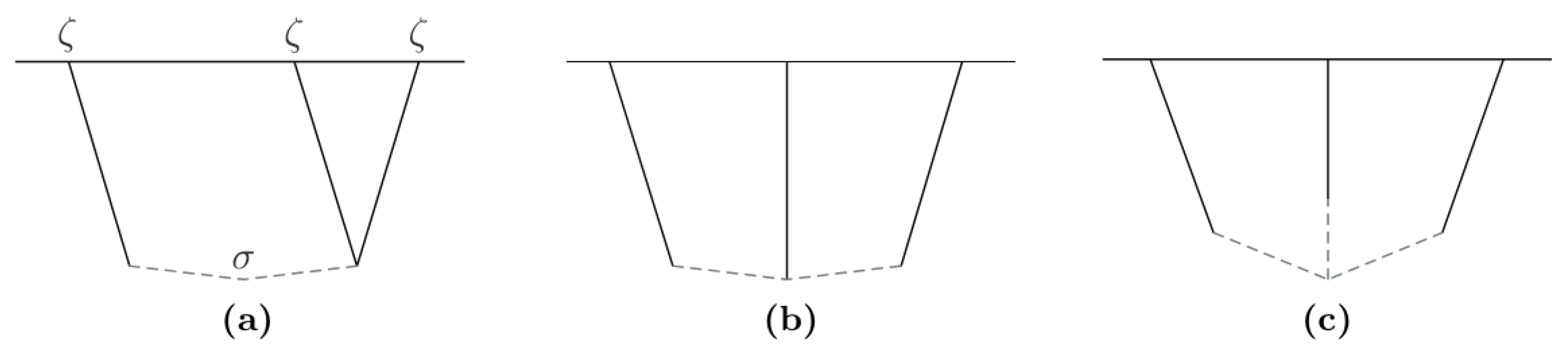
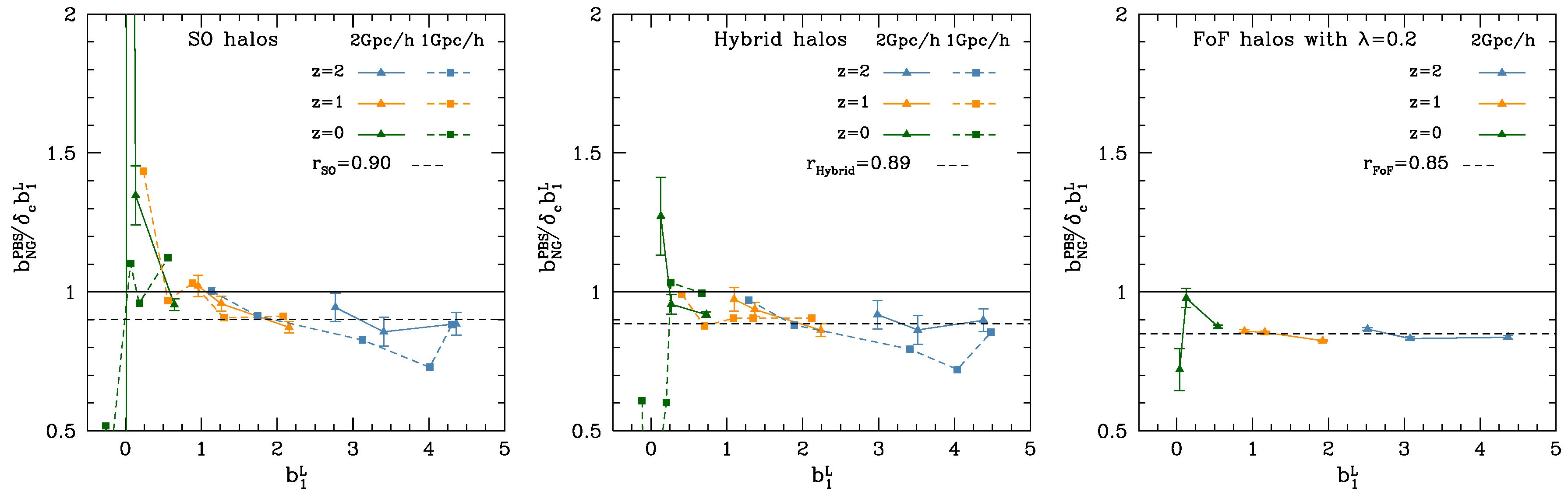
Table 1.
List of values of from the squeezed limit expansion of Equation (150) for interactions produced in single-field models of inflation.
Table 1.
List of values of from the squeezed limit expansion of Equation (150) for interactions produced in single-field models of inflation.
| Interactions in Single-Field Models | ||
|---|---|---|
| Gravitational Floor (Equation (33)) | 0 | |
| DBI (Equation (39)) | ||
| Solid Inflation (Equation (54)) | 0 |
Table 2.
List of values of from the squeezed limit expansion of Equation (150) for interactions produced in multi-field models of inflation. We have parametrized the amplitude of interactions involving the exchange of massive particles using and , where s indicates the spin of the particle, for principal and complementary series, respectively. Full expressions for these amplitudes can be found in [88].
| Interactions in Multi-Field Models | ||
|---|---|---|
| Local (Equation (66)) | 0 | |
| Massive particles | ||
| Even Spin (Principal Series) | ||
| Even Spin (Complementary Series) | ||
| Odd Spin (Principal Series) | ||
| Odd Spin (Complementary Series) |
© 2019 by the author. Licensee MDPI, Basel, Switzerland. This article is an open access article distributed under the terms and conditions of the Creative Commons Attribution (CC BY) license (http://creativecommons.org/licenses/by/4.0/).
Share and Cite
MDPI and ACS Style
Biagetti, M. The Hunt for Primordial Interactions in the Large-Scale Structures of the Universe. Galaxies 2019, 7, 71. https://doi.org/10.3390/galaxies7030071
AMA Style
Biagetti M. The Hunt for Primordial Interactions in the Large-Scale Structures of the Universe. Galaxies. 2019; 7(3):71. https://doi.org/10.3390/galaxies7030071
Chicago/Turabian StyleBiagetti, Matteo. 2019. "The Hunt for Primordial Interactions in the Large-Scale Structures of the Universe" Galaxies 7, no. 3: 71. https://doi.org/10.3390/galaxies7030071
Note that from the first issue of 2016, this journal uses article numbers instead of page numbers. See further details here.