Article

Towards Accurate Prediction of Unbalance Response, Oil Whirl and Oil Whip of Flexible Rotors Supported by Hydrodynamic Bearings

1
Precision and Microsystems Engineering, Delft University of Technology, Mekelweg 2, 2628 CD Delft, The Netherlands
2
Research and Development, Mitsubishi Turbocharger and Engine Europe, Damsluisweg 2, 1332 EC Almere, The Netherlands
3
Institute of Applied Mechanics, Technische Universität München, 85748 Garching, Germany
*
Author to whom correspondence should be addressed.
Lubricants 2016, 4(3), 33; https://doi.org/10.3390/lubricants4030033
Submission received: 31 May 2016 / Revised: 25 August 2016 / Accepted: 5 September 2016 / Published: 8 September 2016

Abstract

:
Journal bearings are used to support rotors in a wide range of applications. In order to ensure reliable operation, accurate analyses of these rotor-bearing systems are crucial. Coupled analysis of the rotor and the journal bearing is essential in the case that the rotor is flexible. The accuracy of prediction of the model at hand depends on its comprehensiveness. In this study, we construct three bearing models of increasing modeling comprehensiveness and use these to predict the response of two different rotor-bearing systems. The main goal is to evaluate the correlation with measurement data as a function of modeling comprehensiveness: 1D versus 2D pressure prediction, distributed versus lumped thermal model, Newtonian versus non-Newtonian fluid description and non-mass-conservative versus mass-conservative cavitation description. We conclude that all three models predict the existence of critical speeds and whirl for both rotor-bearing systems. However, the two more comprehensive models in general show better correlation with measurement data in terms of frequency and amplitude. Furthermore, we conclude that a thermal network model comprising temperature predictions of the bearing surroundings is essential to obtain accurate predictions. The results of this study aid in developing accurate and computationally-efficient models of flexible rotors supported by plain journal bearings.

Graphical Abstract

1. Introduction

Hydrodynamic journal bearings are extensively used in turbomachinery due to their low wear rate and high load-carrying capacity [1]. However, the interaction between the rotating system and the oil film of the journal bearing can cause unstable dynamic behavior characterized by sub-synchronous precessional motion called oil whirl [2]. The whirl frequency of this self-excited motion often increases with rotation speed. For plain journal bearings, the whirl frequency is typically close to half the rotation speed and is superimposed on the synchronous motion originating from residual unbalance. In case the sub-synchronous whirl frequency approaches the natural frequency of an elastic rotor mode, typically at approximately double the first critical speed, oil whip occurs [3]. At rotation speeds beyond the onset speed of oil whip, the whirling frequency no longer increases with rotation speed, but instead locks into the first flexural rotor-bearing mode. As the rotor whirls at a frequency close to the flexural rotor-bearing mode, oil whip is typically characterized by high vibration amplitudes and, therefore, requires careful analysis to prevent excessive wear or even failure of the rotor-bearing system [4,5].
Owing to its interesting and potentially dangerous non-linear behavior, numerous studies focusing on the dynamics of rotors on hydrodynamic bearings have been published [2,6,7,8,9,10,11]. Newkirk and Taylor [12] are regarded to be the first to note that the rotor vibration they observed at approximately double the rotor critical speed was induced by the fluid bearings. Subsequent research on mathematic descriptions of oil whirl showed that the physical fields of the bearing and the rotor have to be analyzed simultaneously [13]. Lund [14] then pioneered the mathematical description of a flexible rotor on fluid film bearings, where he used bearing coefficients based on local linearization of the bearing forces predicted by the Reynolds equation around its static equilibrium condition. This method has mostly been used for stability calculations. Later, when more computation power became available, numerical methods based on time integration became more popular [4].
Subsequent efforts on improving the accuracy of predicting rotor-bearing dynamics have mostly been focused on the bearing models. Features that have been studied are [13,14,15]: cavitation effects, thermal effects, shaft tilting effects, fluid inertia effects, hot oil mixing at the inlet, elastic deformation of the bearing surfaces and non-Newtonian fluid descriptions. Including all of these effects in a model results in computationally-expensive models [16], and hence, simplifying assumptions are adopted, commonly leading to isothermal, fully-aligned short bearing models. However, the accuracy of prediction of the rotodynamic response strongly depends on the validity of the assumptions that are made to create a bearing model. Many of the currently existing experimentally-validated models of rotors on fluid film bearings show significant discrepancies between prediction and measurement in terms of amplitude and onset speeds of oil whirl and oil whip [6,9,10,17].
In this study, we focus on investigating the multiphysical comprehensiveness of a bearing model required to make accurate predictions of the dynamic behavior of a rotor running on fluid film bearings. Therefore, we developed three models with an increasing level of comprehensiveness to study the trade-off between computational accuracy and computation cost. Note that the amount of modeling assumptions decreases with increasing model comprehensiveness. We apply the bearing models to predict the behavior of two different rotor-bearing systems that both encounter oil whirl and oil whip conditions. We also demonstrate the added value of an eigenvalue analysis of the linearized rotor-bearing system to get an indication of the critical speed and the onset of instability. We will show that excessively comprehensive models are computationally heavy, while not necessarily more accurate than more simple models, which make use of well-chosen assumptions.

2. Bearing Models

In this section, three bearing models will be introduced, starting off with a simple bearing model and ending with a comprehensive multiphysical bearing model. The bearing housing and the shaft surface at the bearing location are assumed to be rigid for all three models, as the fluid film pressures are moderate in the evaluated cases. Opposed to the bearing walls being rigid, elastic bending of the shaft is taken into account. Oil is supplied at pressure pi and temperature Ti on top of the bearing; see Figure 1. At the axial ends of the bearing, the oil flows out at ambient pressure. All three bearing models are based on the Reynolds equation, which assumes laminar flow, neglects fluid inertia effects and assumes constant pressure throughout the height of the oil film due to the small oil film thickness. The pressure distribution in a thin lubricating film with film thickness h, which supports a shaft with radius R at rotation speed Ω, is described by:
x h 3 ρ 12 μ p x + Ω R h ρ 2 + z h 3 ρ 12 μ p z + h ρ t = 0
where μ and ρ denote the lubricant viscosity and density, respectively. x represents the circumferential coordinate x = θ R , and z indicates the axial coordinate. When perfect shaft alignment is assumed, the expression for the film thickness h as a function of the angle θ may be written as:
h = C e X cos ( θ ) e Y sin ( θ )
where C is the nominal radial clearance and e X and e Y are the displacements from the center position in the global, non-rotating reference frame, as depicted in Figure 1.

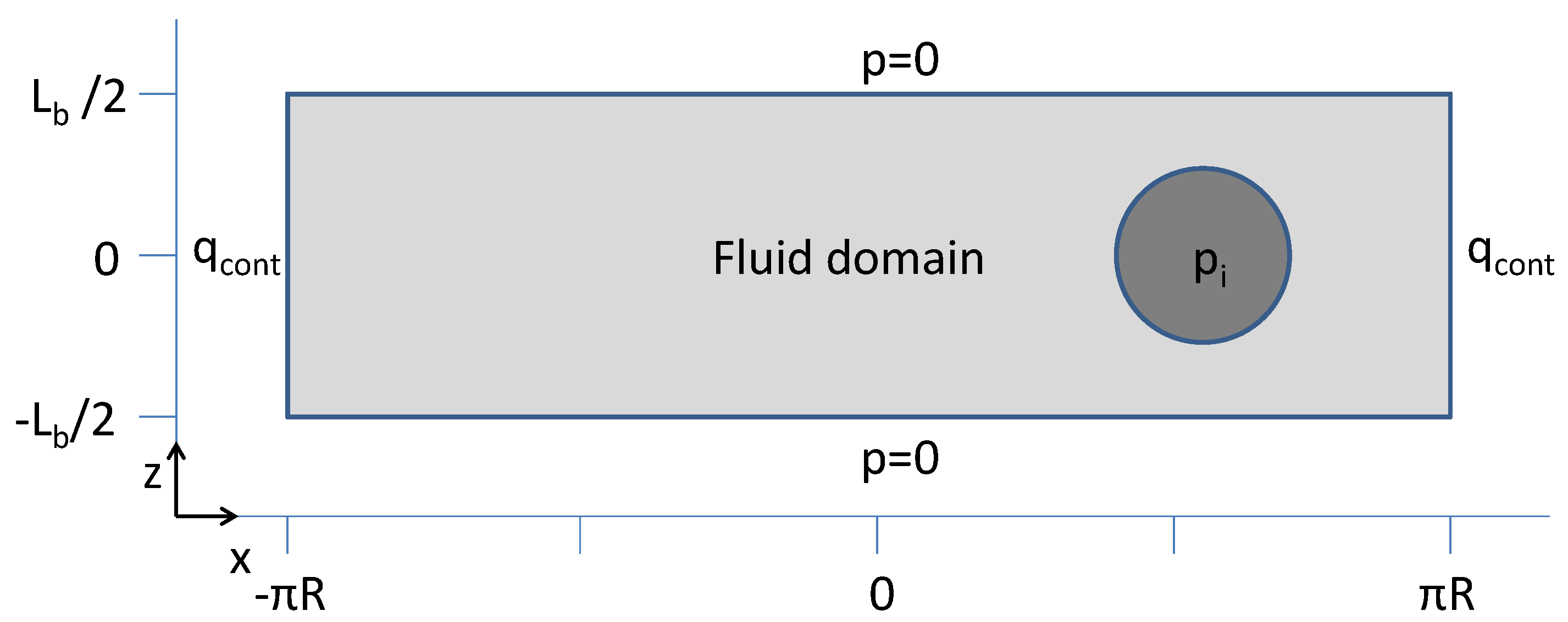
2.1. Bearing Model 1: Isoviscous Short Bearings with Half-Sommerfeld Cavitation Conditions.

For the first bearing model, we apply the following assumptions:
  • the flow is dominated by the pressure gradients in the axial direction, and thus, the pressure gradient in circumferential direction can be ignored: p x p z .
  • the fluid viscosity does not vary with time or location.
  • the shaft is always aligned with the bearing bore, i.e., shaft tilting is not included in the fluid film thickness function.
  • the pressure distribution is dominated by the hydrodynamic pressure buildup; therefore, the hydrostatic pressure contribution of the supply is neglected.
Based on these assumptions, an analytical expression for the pressure distribution can be obtained. Integrating this expression over the bearing circumference and discarding negative pressures in the cavitated areas (half-Sommerfeld boundary conditions), a closed form expression of bearing reaction forces in radial and tangential directions is [18]:
F r = μ R L b 3 2 C 2 2 ε 2 Ω 2 Θ ˙ 1 ε 2 2 + π ε ˙ 1 + 2 ε 2 1 ε 2 5 / 2 F t = μ R L b 3 2 C 2 π ε Ω 2 Θ ˙ 2 1 ε 2 3 / 2 + 4 ε ε ˙ 1 ε 2 2
where L b is the bearing length, Θ ˙ is the whirl velocity of the bearing and ε is the dimensionless eccentricity ratio ε = e X 2 + e Y 2 h 0 . The radial force F r acts along the instantaneous attitude angle Θ, whereas the tangential force F r acts along Θ, where:
Θ = tan 1 e Y e X
These bearing forces can be transformed to the stationary inertial coordinate system XY:
F b = F X F Y = sin ( Θ ) cos ( Θ ) cos ( Θ ) sin ( Θ ) F r F t
This bearing model, which gives a reaction force as a function of the bearing design and operating conditions, will be used to evaluate two different rotor-bearing systems in Section 3 and Section 4.

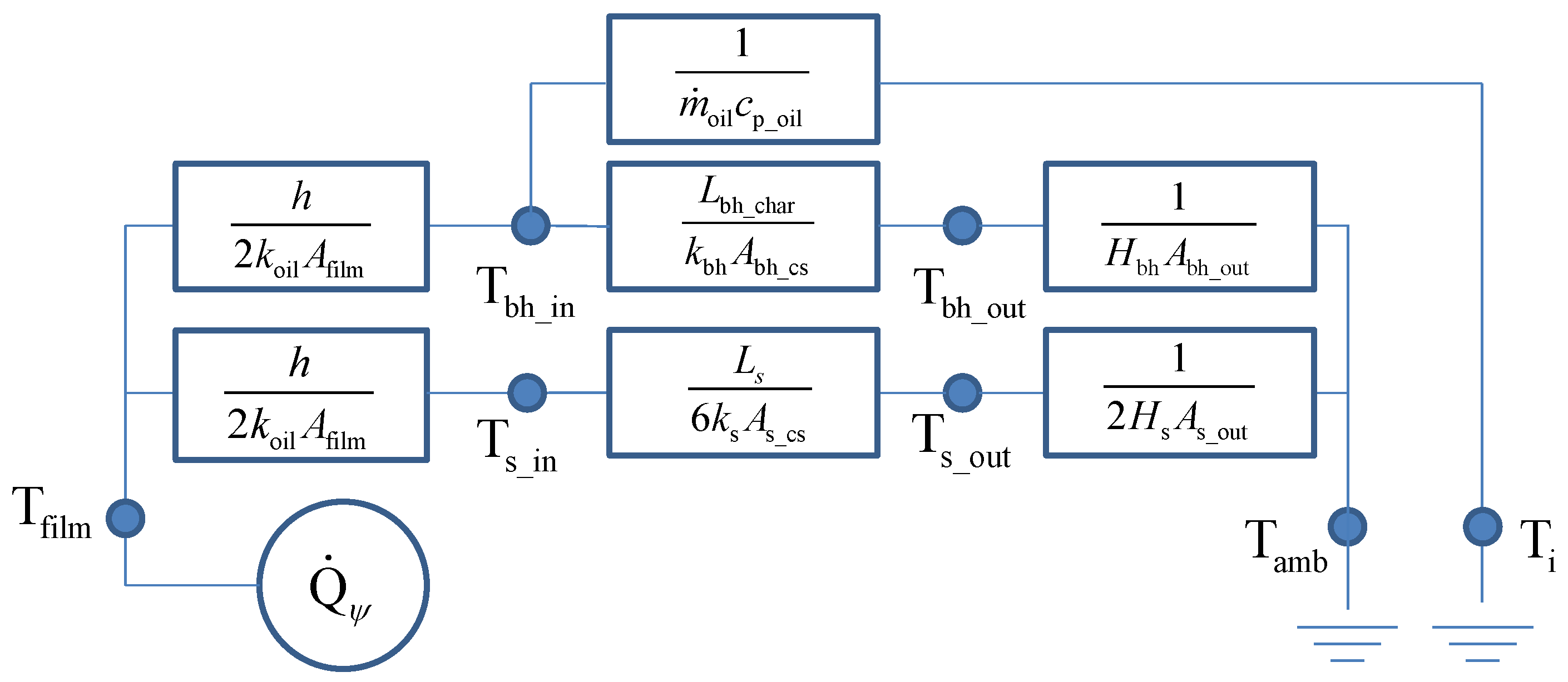
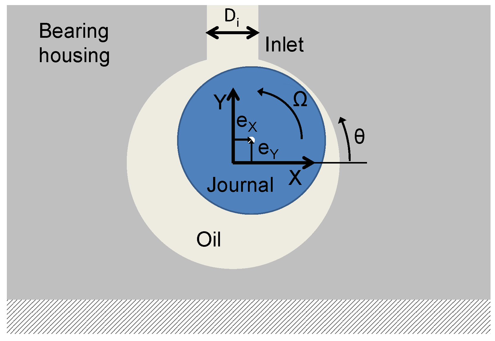
2.2. Bearing Model 2: Finite Length Journal Bearing with Gümbel Cavitation Conditions Including a Lumped Thermal Model

In Model 1, a short bearing model is used, which assumes that the circumferential flow is much smaller than the axial flow and can thus be omitted from the Reynolds equation in order to derive the explicit expression of Equation (3). This assumption can be made when the bearing is narrow, i.e., L b / 2 R < 1 / 2 [2]. In case the bearing is not particularly narrow nor long, the Reynolds equation needs to be solved in two directions, which is done in Model 2. In this model, we use a finite element discretization scheme [19] to solve Equation (1) over the fluid domain depicted in Figure 2.
Gümbel cavitation conditions are imposed by setting negative pressures from the solution of Equation (1) to zero using a Boolean function:
p * = ( p 0 ) p
where the term ( p 0 ) is equal to one for non-negative pressures and zero for negative pressures. The influence of Gümbel cavitation conditions on the rotodynamic response of a Laval rotor have been investigated by Nitzschke [20] who obtained fairly similar results using either Elrod-like or Gümbel cavitation conditions.
The shear losses in the oil film cause an increase in oil temperature T film and consequently a decrease in viscosity μ [4]. Therefore, a lumped thermal model is taken into account in Model 2. The thermal model is based on an energy balance of the rotor-bearing system, including the bearing housings, as shown in Figure 3. The friction heat Q ψ , which is generated in the fluid film, partly exits the bearing by heating the lubricant, which flows through the bearing m ˙ oil , and partly by heat conduction and convection from the lubricant to the rotor and the bearing housing. Figure 4 shows the thermal network in which only steady state components are included, as quasistatic run-up or run-down conditions are assumed: the time constant for the shaft motion is considerably smaller than the time constant involved in the thermal behavior of the rotor-bearing system.
In the thermal network model, the friction in the fluid film Q ψ originates from pressure extrusion losses and from shear flow losses and is calculated by:
Q ψ = L / 2 L / 2 π R π R ( p 0 ) h 3 12 μ p x 2 + p z 2 + ( p 0 ) μ Ω R 2 h d x d z
Heat flow from the fluid film to its surroundings can be modeled by solving the energy equation in three directions, as done by Mahner et al. [21], or alternatively by assuming an average temperature at the center of the height of the fluid film [22]. For this model, we assume the latter in order to keep the computational effort at a minimum during time-transient simulations of the rotor-bearing system. The heat transfer from the fluid film to the shaft and the bearing housing is therefore represented as conduction from halfway of the film height h / 2 , as depicted in Figure 4.
The heat going into the bearing housing is partly transferred to ambient air and is partly transferred to the oil in the inlet channel upstream the film. It is observed that most of the temperature increase of the oil actually occurs here and not in the oil film itself. The amount of heat leaving the bearing via the oil flow thus depends on T bh _ in T i and the instantaneous mass flow of oil:
m ˙ oil = π R π R n z ( p 0 ) ρ h 3 12 μ p z z = L b / 2 L b / 2 d x
where n z is the vector normal to the edges of the bearing.
Conduction through the shaft is assumed to occur on two sides of the bearing up to a point 1 / 3 of the shaft half-length L s / 2 at each side of the bearing, where the temperature is halfway of its decay from T s _ in . Subsequently, convection takes place from the rotating shaft, estimated by [23]:
H shaft = k air 15 R R e air 2 / 3 P r air 1 / 3
where the Reynolds number R e air depends on the rotation speed and the kinematic viscosity of air ν air :
R e air = 4 Ω R 2 ν air
Convection from the bearing housing outer surface A bh _ o occurs by natural convection: H bh = H free .
The lumped film temperature T film is determined by balancing the friction losses in the bearing with the amount of heat carried away by the oil and transferred to the bearing housing and the shaft:
Q ψ ( μ ( T film ) ) Q via _ oil Q via _ bh Q via _ shaft = 0
This balance is iteratively found by finding the temperature T film using the relation between oil viscosity and temperature described by the Vogel equation [4]:
μ ( T film ) = a e b T film + c
using the constants a, b and c corresponding to the specific type of oil; see Table 1 and Table 2. The thermal network model was compared with the results of a conjugate heat transfer model, where the predictions of both models were in good correspondence, with maximum deviations of 3 K.
The thermal balance of Equation (11) is solved together with the Reynolds equation (Equation (1)) over the fluid domain depicted in Figure 2. The bearing reaction forces can then be calculated by integrating the pressure over the bearing domain:
F X = L b / 2 L b / 2 π R π R p * cos θ d x d z F Y = L b / 2 L b / 2 π R π R p * sin θ d x d z
Contrary to Model 1, Model 2 does not assume that the viscosity is independent of time, as the lumped oil viscosity changes with the operating conditions. Furthermore, the Reynolds equation is solved in two dimensions instead of one, so that we no longer have to neglect the pressure gradient in the circumferential direction. In addition, the hydrostatic pressure from the supply is taken into account in Model 2. The most important remaining assumptions in Model 2 are that the viscosity does not vary with location and that the shaft is always aligned in the bearing housing.

2.3. Bearing Model 3: Finite Length Journal Bearing Including a Mass-Conservative Cavitation Algorithm, Non-Newtonian Fluid Description, Shaft Tilting Kinematics and a Distributed Thermal Model

Model 3 can be seen as an extension to Model 2 as the Reynolds equations are again solved on the fluid domain depicted in Figure 2. This time, however, the modeling is more comprehensive, and therefore, the number of assumptions is further reduced, as will be explained in this section.
Model 1 and Model 2 truncate negative pressures to zero to prevent the pressure distribution from containing negative pressures. This approach, however, is not mass conservative and can therefore lead to inaccurate results, especially for thermal models where conservation of mass can be important [24]. Hence, in the third model, a mass conservative cavitation algorithm is used. The cavitation algorithm is incorporated in the Reynolds equation by including the mass fraction f and by substituting p by ξ P 0 :
q x x + q z z + h f ρ t = 0
where:
q x = ρ f h 3 12 μ ξ x P 0 + Ω R f h ρ 2 q z = ρ f h 3 12 μ ξ z P 0 P 0 = μ 0 Ω R 2 C
The mass fraction f is defined such that it equals one in the full film area and represents the mass fraction 0 f 1 when the film is cavitated:
f ( x , z ) = 1 + ξ ( ξ < 0 ) c f
in which c f is a transformation coefficient that arises from a flow balance in the circumferential direction under the assumption of streamer cavitation; see Alakhramsing [24] for details. The physical pressure p can be calculated by:
p = ξ ( ξ 0 ) P 0
The expressions ( ξ < 0 ) and ( ξ 0 ) are Boolean functions, which are one when true and zero otherwise. The cavitation algorithm of Alakhramsing was proven to be computationally efficient and robust for THDsimulations [24] and was therefore selected over alternative mass conservative cavitation algorithms.
In Model 2, the viscosity of oil was assumed to be only dependent on temperature. The viscosity of multi-grade oils, as often used for plain journal bearings, also depends on the local film shear rate γ ˙ :
γ ˙ = Ω R h .
At high shear rates, the viscosity decreases. This non-Newtonian effect is often referred to as shear thinning [4]. In Model 3, the viscosity formulation of Model 2 is therefore extended by including shear rate dependency according to the Cross equation [25]:
μ ( T film , γ ˙ ) = a e b ( T film + c ) r + 1 r 1 + ( K γ ˙ ) m
with the parameters r, m and K corresponding to the specific type of oil; see Table 1 and Table 2.
Models 1 and 2 assume that the shaft is always aligned with the bearing housing. When shaft misalignment occurs due to shaft bending or shaft tilting, the film height varies over the axial direction, so Equation (2) is no longer sufficient. In Model 3, a shaft tilting description is included by adding tilting terms to the original film height description of Equation (2) [26]:
h = C 1 z sin φ Y + e X cos ( θ ) z sin φ X + e Y s i n ( θ )
where φ X and φ Y represent the tilting angles of the beam in the X and Y direction, respectively, at the center of each bearing. This description allows the peak film pressures to occur off the centerline of the bearing. In addition to the forces, which are calculated by Equation (13), a resulting torque acts on the shaft at the bearing locations:
M X = F X L b / 2 L b / 2 π R π R p * z d x d z L b / 2 L b / 2 π R π R p * d x d z M Y = F Y L b / 2 L b / 2 π R π R p * z d x d z L b / 2 L b / 2 π R π R p * d x d z
The friction loss ϕ over the bearing surface per unit area arises from both pressure work and shear losses:
ϕ = ξ > 0 h 3 12 μ ξ P 0 x 2 + ξ P 0 z 2 + f μ h
where the shear losses are assumed to occur in the full film area, as well as in the ratio f of the cavitated area under the assumption of finger-type cavitation.
The thermal model of Model 3 connects to the same thermal network as Model 2, depicted in Figure 4, but instead of having a lumped film temperature T f i l m , the temperature within the fluid film varies over the x-z-domain. The thermal distribution over the film domain is described by conduction and convection in the x and z direction, thermal storage, friction heat generation ϕ and heat transfer to the surroundings as follows:
x f k oil h T x + c p q x T + z ( ξ > 0 ) k oil h T z + c p q z T + ρ c p _ oil h T t = . . . . . . ϕ 2 f k oil h 2 T T shaft _ in T bh _ in
As finger-type cavitation is assumed, the fluid in the cavitated region forms streamers so that the conduction of heat in the z direction can only occur in the full film region, hence the term ( ξ > 0 ) in Equation (23). Moreover, conduction in the x direction will only occur at the fraction of fluid f.
At the axial ends of the film domain, the constant pressure boundary condition of Model 2 is replaced by a non-submerged boundary condition, which allows the flow to exit the domain, but prevents it from re-entering [24]:
ξ 0 q z n z > 0 L / 2 L / 2
In this model, the fluid and thermal equations, Equations (14) and (23), are simultaneously solved using a modified Newton–Raphson iteration scheme.

2.4. Summary of Bearing Models

Table 3 summarizes this section by giving an overview of the details of the three bearing models.
Having developed three increasingly comprehensive bearing models, we will now evaluate their performance using two case studies in the subsequent sections.

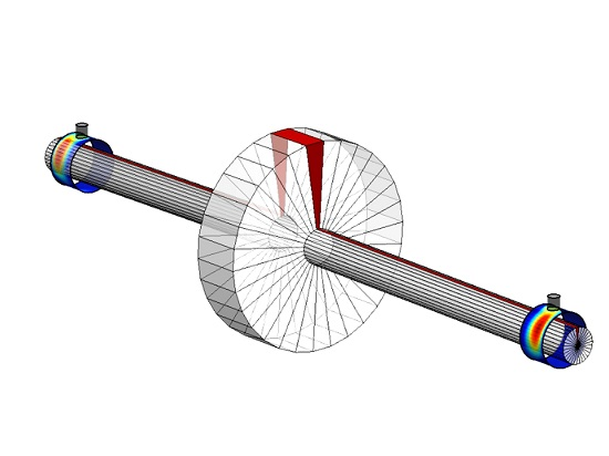
3. Rotor-Bearing System A: A High Speed Laval Rotor on Plain Journal Bearings

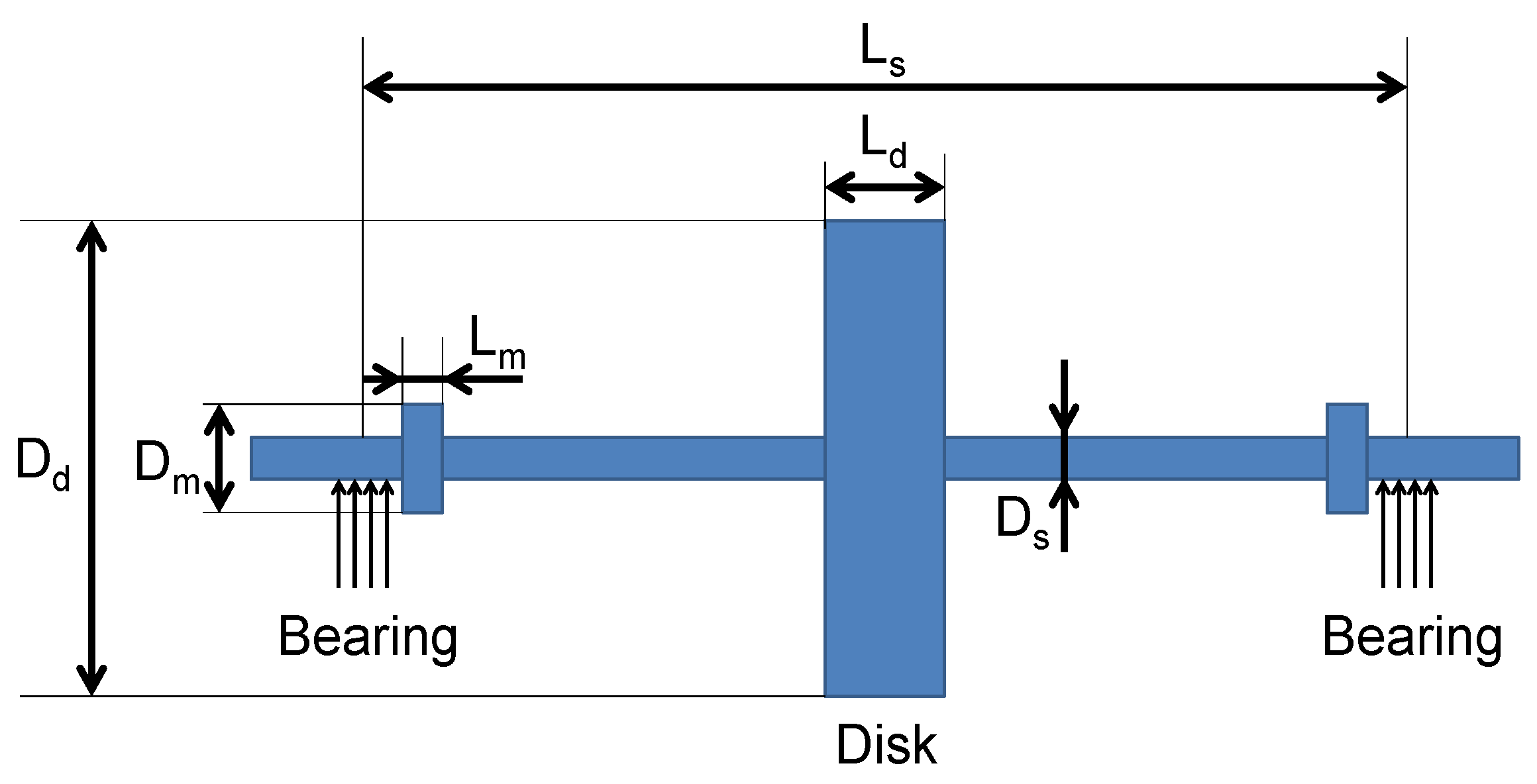
3.1. Rotor and Bearing Layout

The first rotor-bearing system (rotor-bearing System A) consists of a simple symmetric rotor supported by plain journal bearings; see Figure 5. This rotor is essentially a Laval rotor, with two small disks adjacent to the main disk, which were added to facilitate the use of two eddy current sensors in orthogonal radial directions [16]. The rotor-bearing system is based on an example provided by Schweizer [8] and is described by the parameters given in Table 1. The rotor is driven by an electric motor via a lightweight compliant coupling. A more detailed description of the rotor-bearing system and the experimental setup can be found in [16].

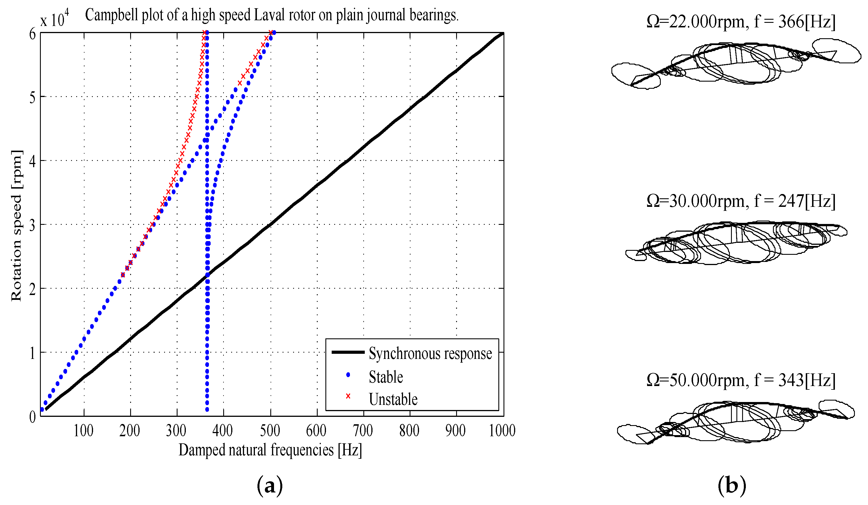
3.2. Rotor Model and Linear Rotodynamic Response

In order to get a global understanding of the rotor-bearing behavior, a linear rotodynamic analysis is a quick and insightful first step. The rotor itself is modeled using a finite element model using Rayleigh beam elements and disk elements, including the gyroscopic terms for both element types. Small displacements on a slender rotor are studied; therefore, the Rayleigh beam was considered to be adequate. Furthermore, material damping of the rotor is modeled by Rayleigh damping. The non-rotating rotor model was validated by hammer impact tests: the eigenfrequencies in the synchronous operating range were correctly predicted within 3% of the measured values.
For the linear rotodynamic analysis, we make use of a bearing formulation similar to that of Model 1; however, we further simplify Equation (3) by assuming steady operating conditions. This leads to the elimination of the whirl and squeeze-dependent terms:
F r = μ R L 3 Ω ε 2 C 2 1 ε 2 2 F t = μ R L 3 π ε Ω 4 C 2 1 ε 2 3 / 2
Based on these expressions, the 2 × 2 linearized stiffness and damping matrices of each bearing can be derived; see Hamrock [27] for details. An eigenvalue analysis of the linear rotor-bearing system is performed, resulting in the Campbell plot of Figure 6a and the associated mode shapes in Figure 6b.
A typical response of a flexible Laval rotor on plain journal bearings is predicted:
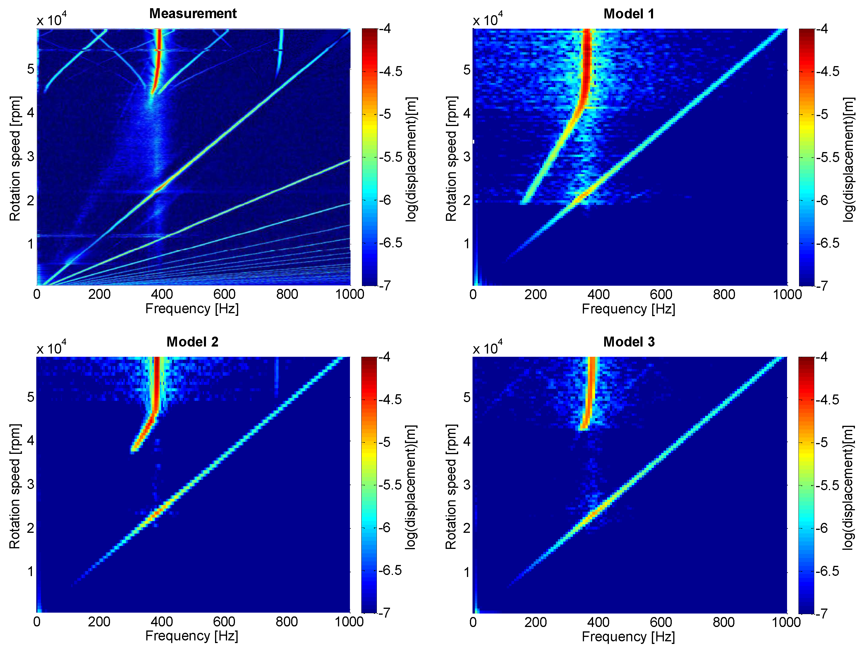
  • traversal of a critical speed caused by the first shaft bending mode at Ω c r i t i c a l = 366 Hz.
  • above this critical speed, the first rigid body mode (a cylindrical mode, see Figure 6b) becomes linearly unstable at Ω whirl = Ω critical / 2 = 183 Hz.
  • at rotation speeds above 40.000rpm, the whirl locks into the first shaft bending mode, resulting in a whip mode, which combines rigid body motion and bending motion.
Furthermore, a second whirling mode is predicted to become unstable around 52.000 rpm. This is the conical mode of the shaft, a pure rigid body whirl.

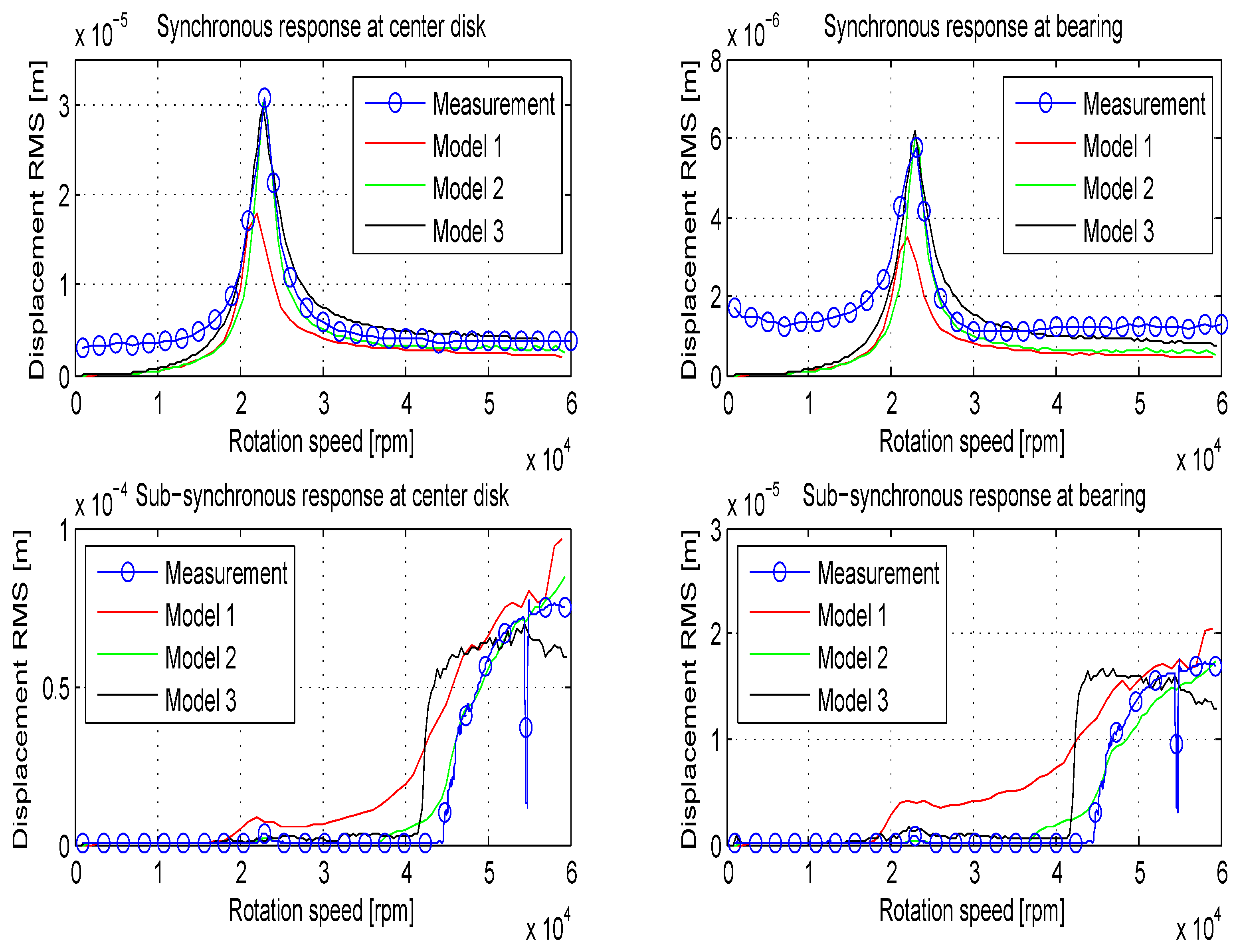
3.3. Non-Linear Time-Transient Analysis

After having performed the linear rotodynamic analyses, the next step is to perform non-linear time-transient analysis. To that end, we coupled the rotor model, as described and analyzed in Section 3.2, to the bearing models described in Section 2 and performed a run-up from 1000 rpm to 60.000 rpm in 120 s. The bearings are supplied with oil at a pressure of 2.8 bar and a temperature of 25 °C, which is also the ambient temperature. An unbalance amount of 250 mg·mm was applied on the central disk. For Model 1, a constant fluid temperature of 320 K was assumed, which is the average lumped film temperature predicted by Model 2. The resulting equations of motion can be written as:
M q ¨ + ( C + G ( Ω ) ) q ˙ + Kq = F
where the matrix M represents the mass matrix, C represents the damping matrix, G represents the gyroscopic matrix and K represents the stiffness matrix. F contains the bearing forces and the unbalance forces. Lastly, the vector q contains the global generalized displacements. A Newton–Raphson algorithm solves the fully-coupled system of equations describing the rotor-bearing system. The model contains 8800 degrees of freedom, and convergence is accepted at a relative error of 10 4 .
The resulting runup data are displayed in Figure 7: waterfall plots of the response on the measurement disk adjacent to the bearing of the experimental results compared with the predictions of the three different rotor-bearing models. The measurement shows the occurrence of a critical speed traversal around Ω critical = 380 Hz. A sub-synchronous whirl starts at a rotation speed of 44.000 rpm at a frequency of approximately Ω whirl = 360 Hz. At rotation speeds over 50.000 rpm, the whirl locks into the first shaft bending mode to form a whip at Ω whirl = 380 Hz.
The three numerical models correctly predict the occurrence of the critical speed traversal and the occurrence of a whirl, which locks into the first bending mode. Looking closer, we see that the main difference between the results of the three models is that the onset of the whirl is underpredicted by the numerical models. Especially Model 1, which does not take the hydrostatic feed pressure into account, predicts a whirl to start already around 20.000 rpm. Model 2 shows better resemblance by predicting the whirl to start around 37.000 rpm and shows a clear transition from whirl to whip conditions. Model 3, which is the only model that captures the effects of shaft tilting and shear thinning of the lubricant, shows even better resemblance with the measurement results, as the whirl is predicted to start beyond 40.000 rpm, as observed during measurements.
Figure 8 gives the measured RMS-values of synchronous and sub-synchronous displacement for both the locations near the bearing, as well as on the center disk compared with the model predictions. All data were filtered using bandpass filters for the synchronous component 0.9 f synch < f < 1.1 f synch and the sub-synchronous component 0.1 f synch < f < 0.9 f synch .
Considering the synchronous response, we see that the frequency of the critical speed is generally well predicted by the three models. At low rotation speeds, the experiment shows some unpredicted response, most likely coming from residual out-of-plane unbalance. At the critical speed, Model 2 and Model 3 give accurate predictions within 5% of the measured values. The peak amplitude of Model 1 is clearly smaller than those of the other two models, most likely due to the short bearing formulation of Model 1, which overpredicts the pressures so that the eccentricities are underpredicted.
Considering the sub-synchronous response, the models underpredict the whirl onset speed, where Model 1 is clearly most off, followed by Model 3 and then Model 2. The amplitude of the whirl is relatively well predicted by the three models. Overall, Model 2 seems to correlate at least as well with the measurement data as Model 3 in terms of whirl amplitude.
Comparing these results with our previous study [16], a much better correlation between measured response and predicted response is found. This may be attributed to two major model improvements:
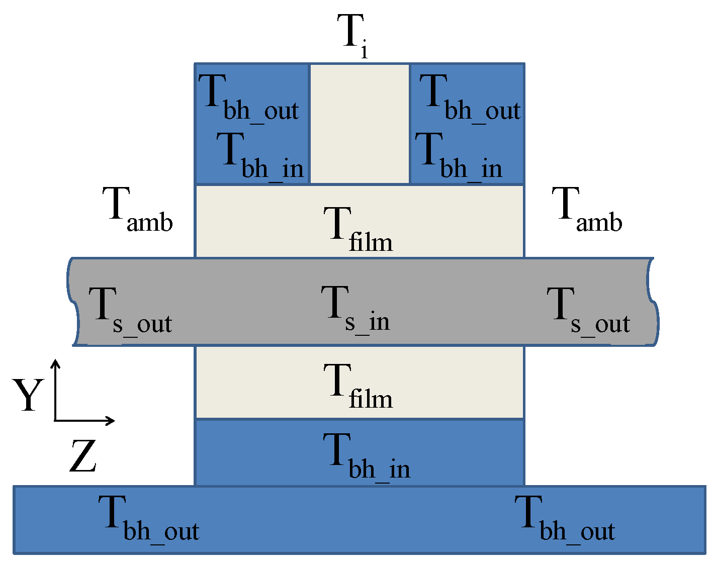
  • the extension of the thermal model to include the heating of the shaft, the bearing housing and the oil in the inlet channel, as depicted in Figure 4. Especially the effect of heating the oil in the inlet channel inside the bearing housing just upstream the bearing was found to be having a major impact on the effective film temperature.
  • it was found by experiments on a viscometer that the oil viscosity-temperature parameters used in our previous study [16] were incorrect. The newly-found oil viscosity-temperature parameters can be found in Table 1.
The computation times for the three models are respectively 1 h, 6 h and 30 h on a 3.6-GHz Xeon computer: the increase of model comprehensiveness clearly comes at a cost. The mesh of the models was checked to be mesh-converged, based on the peak pressure in the fluid film.

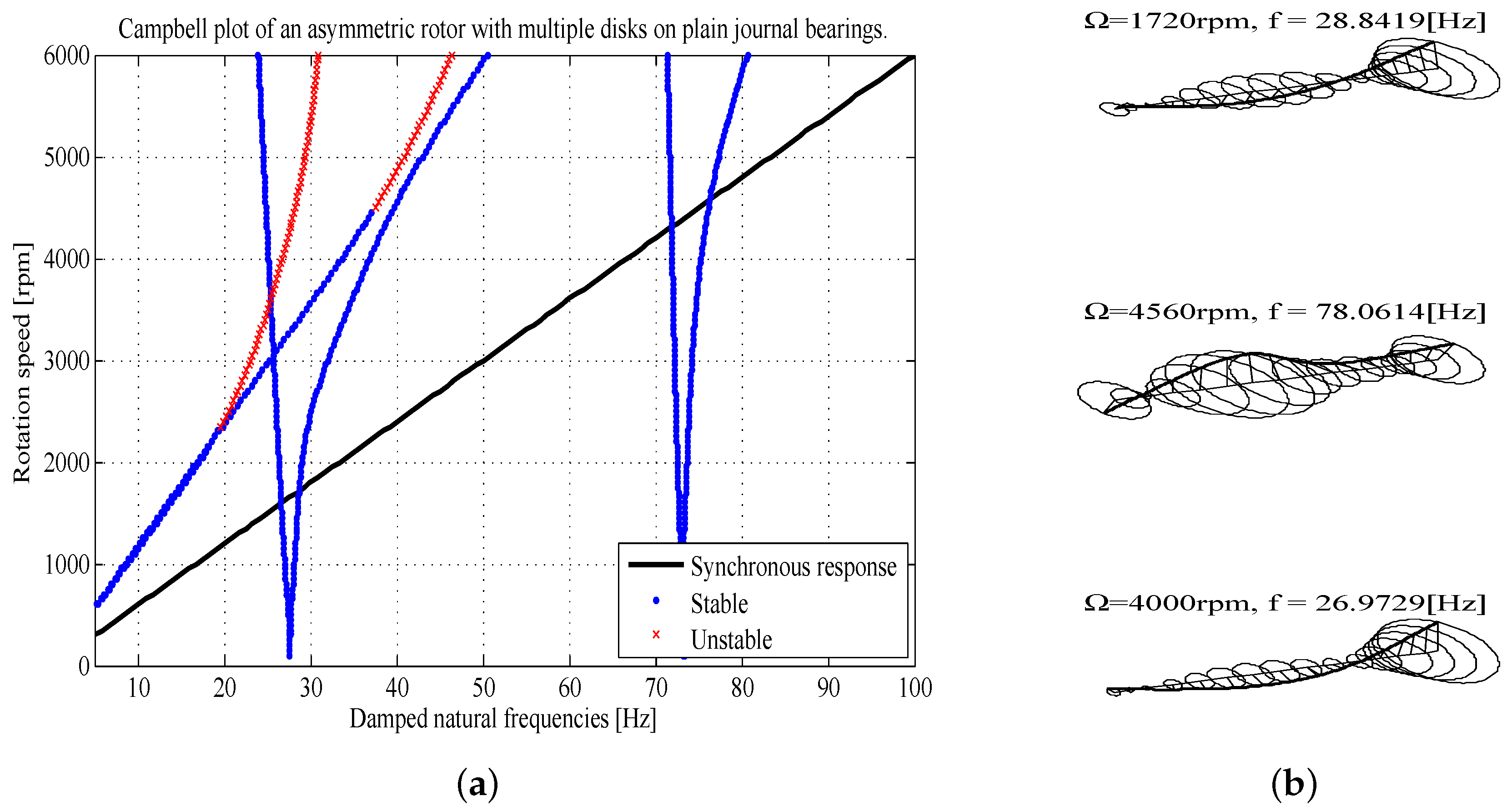
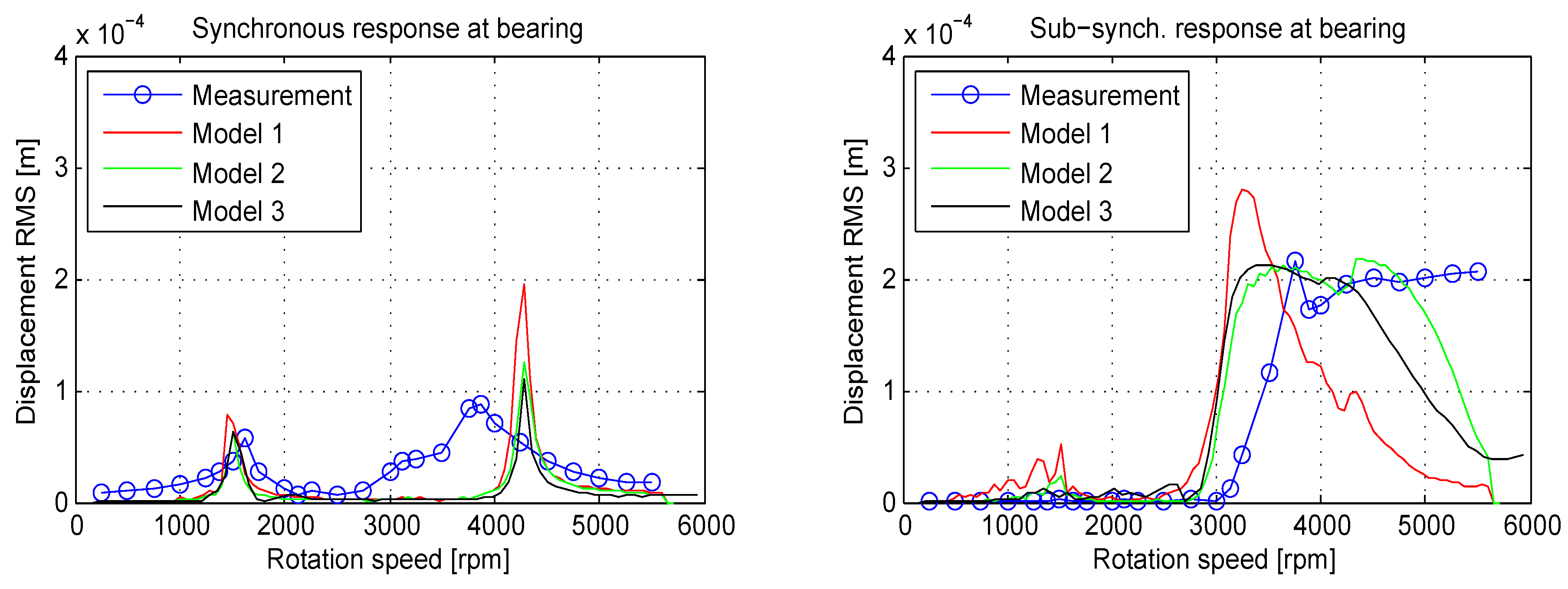
4. Rotor-Bearing System B: An Asymmetric Rotor with Multiple Disks on Plain Journal Bearings

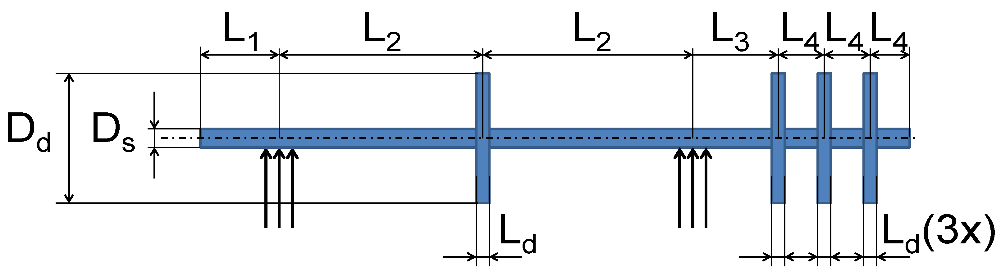
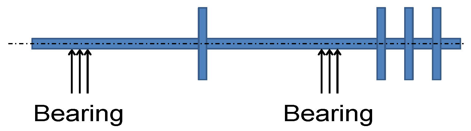
4.1. Rotor and Bearing Layout

The second test case for our study is the rotor-bearing system used by El-Shafei [28], who experimented with a rotor-bearing system consisting of a central disk and three overhung disks on a shaft, which is supported by plain journal bearings; see Figure 9. This system has a completely different geometry and operating speed from rotor-bearing System A and is particularly interesting because more than one critical speed is traversed. In addition, due to the overhung disk configuration, shaft tilting is expected to be more pronounced compared to rotor-bearing System A. Details of the rotor-bearing system can be found in Table 2.

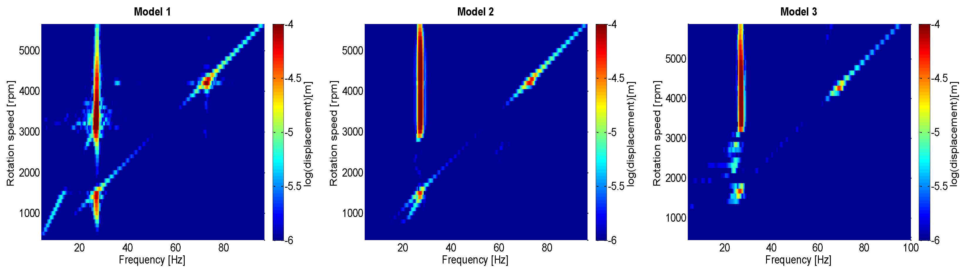
4.2. Linear Analysis: Campbell Plot

Analogous to Section 3.2, an eigenvalue analysis of the linearized rotor-bearing system is performed. The results in Figure 10a show that this rotor traverses two critical speeds and that several sub-synchronous modes exist.

4.3. Non-Linear Time-Transient Analysis

Analogous to Section 3.3, non-linear time-transient analyses have been performed with bearing Models 1 to 3 for rotor-bearing System B. The test conditions are: p i = 4 bar, T i = 25 °C. An unbalance of 189 g·mm is added to the central disk. These conditions correspond to Case 3 described by El-Shafei [28]. Figure 11 shows the comparison between the measurement results, kindly provided by Prof. El-Shafei, and the results of our models, both on the basis of the synchronous and sub-synchronous response data. The measurement, as well as the simulations were performed in run-down conditions from 5500 rpm to 250 rpm. As a side note, it can be mentioned that the whirl showed hysteresis: the onset speed of whirl was considerably higher during run-up simulations than during run-down simulations. In this study, only run-down conditions are considered.
Figure 11 presents the synchronous and sub-synchronous displacement near the left-hand bearing. The synchronous responses of all three models are similar. The first critical speed prediction is close to the measurement result; however, the second critical speed traversal is 400 rpm higher than measured. It is believed that the mass of the rotor-motor coupling element in the test setup had a considerable influence on this mode, causing a decreased critical speed on the test setup. The mass and stiffness of this coupling are, however, not included in the models.
As for the sub-synchronous response, the models underpredict the onset speed of whip by 500 rpm typically. This could be caused by the influence of the coupling on the rotor-bearing dynamics. Furthermore, it was checked that the change of clearance due to different thermal expansion of the shaft and the bearing was less than 0.5 micrometers, so it may be neglected. The thermal interaction between the bearings have not been included in our models; this could be a reason for the discrepancy between the simulation results and the measurement results.
Figure 12 gives a comparison of the model results in the frequency domain. Unfortunately, insufficient measurement data were available to construct a similarly accurate waterfall plot of the experimental results. Based on the available data, however, it can be concluded that a reasonable correlation with the whirling frequencies is found: El-Shafei [28] measured whirling frequencies in the range of 28 Hz–30 Hz, whereas the models predict whirling frequencies of 29 Hz–32 Hz.
The computation times for the three models are respectively 0.6 h, 4 h and 22 h on a 3.6-GHz Xeon computer.

5. Conclusions

Coupled simulation of rotor dynamics, fluid film dynamics and rotor-bearing thermodynamics results in accurate prediction of unbalance response, oil whirl and oil whip of flexible rotors supported by hydrodynamic bearings, provided that all relevant physics are adequately included in the model. A simple isothermal linearized rotor-bearing model can already provide a good indication of the response to be expected and is a quick, yet insightful tool compared to more comprehensive multiphysical time-transient simulations. As the behavior of these rotor-bearing systems is strongly non-linear and multiphysical, non-linear rotor-bearing models should be used when more accurate predictions of the rotor response are required.
Regarding the comprehensiveness of modeling fluid bearings: based on the two considered rotor-bearing systems, we conclude that a thermal network model that includes temperature predictions of the bearing housing surface, the shaft surface and the oil temperature at the inlet of the bearing is required to obtain accurate predictions of the rotor-bearing response. The added value of a distributed thermal model within the fluid film compared to a lumped thermal model is very limited. Likewise, the added value of a mass conservative cavitation algorithm over non-mass conservative boundary conditions is also very limited. In the investigated cases, the change of shear rate over the operating range is considerable; therefore, the non-Newtonian fluid description is regarded to be important. The effect of shaft-misalignment was negligible in both cases. The hydrostatic pressure of the oil feed channel increases the onset speed of whirl and is therefore an important effect to take into account.
The increase of modeling comprehensiveness comes with an increase in computational cost. It is therefore wise to simplify the rotor-bearing model as much as possible, as long as the required assumptions necessary for simplification are valid. The development of sufficiently-comprehensive rotor-bearing models results in accurate and fast predictions, leading to optimal rotor-bearing performance and first-time-right designs.

Author Contributions

Rob Eling and Mathys te Wierik developed the rotor-bearing models, constructed the test setup and conducted the experiments of rotor-bearing system A. Rob Eling wrote the manuscript. Ron van Ostayen and Daniel Rixen assisted in the model development and supervised this work.

Conflicts of Interest

The authors declare no conflict of interest.

Appendix A. Numerical Values of Rotor-Bearing System A

Table A1. Thermal network parameters of rotor-bearing System A.
SymbolDescriptionValueUnitSymbolDescriptionValueUnit
A b h _ c s Cross-sectional area bearing housing3e 4 m 2 k o i l Thermal conductivity of oil0.145 W m K
A b h _ o Outer surface area bearing housing6e 3 m 2 k s h a f t Thermal conductivity of shaft44 W m K
H b h Convection coefficient from bearing housing5 W m 2 K L c h a r _ b h Characteristic length of conductance in bearing housing1.14e 2 m
k a i r Thermal conductivity of air2.8e 2 W m K ν a i r Kinematic viscosity of air17e 6 m 2 s
k b h Thermal conductivity bearing housing201 W m K c p _ o i l Specific heat of oil2.1e 3 J k g K
P r a i r Prandtl number of air0.69

Appendix B. Numerical Values of Rotor-Bearing System B

Figure B1. Schematic of Rotor B.
Lubricants 04 00033 g013
Note: the disks in the rotor contain twelve 8 mm-diameter holes in the axial direction on a 140 mm-diameter circle. Furthermore, the bearing contains two inlet holes for oil supply instead of one, these inlets are located at θ = π / 3 and θ = 2 π / 3 . Further details can be found in the paper of El-Shafei [28].
Table B1. Thermal network parameters of rotor-bearing System B.
SymbolDescriptionValueUnitSymbolDescriptionValueUnit
A b h _ c s Cross-sectional area bearing housing6e 4 m 2 k o i l Thermal conductivity of oil0.145 W m K
A b h _ o Outer surface area bearing housing5e 2 m 2 k s h a f t Thermal conductivity of shaft44 W m K
H b h Convection coefficient from bearing housing5 W m 2 K L c h a r _ b h Characteristic length of conductance in bearing housing2.9e 2 m
k a i r Thermal conductivity of air2.8e 2 W m K ν a i r Kinematic viscosity of air17e 6 m 2 s
k b h Thermal conductivity bearing housing44 W m K c p _ o i l Specific heat of oil2.1e 3 J k g K
P r a i r Prandtl number of air0.69

References

  1. Friswell, M.I.; Penny, J.E.T.; Garvey, S.D.; Lees, A.W. Dynamics of Rotating Machines; Cambridge University Press: Cambridge, UK, 2010. [Google Scholar]
  2. San Andrés, L. Modern Lubrication Theory, Lecture Notes 5: Dynamics of Rigid Rotor-Fluid Film Bearings Systems. Available online: http://rotorlab.tamu.edu/me626/default.htm (accessed on 8 September 2016).
  3. Poritsky, H. Contribution to the Theory of Oil whip. Trans. ASME 1953, 75, 1153–1161. [Google Scholar]
  4. Stachowiak, G.; Batchelor, A.W. Engineering Tribology, 4th ed.; Butterworth-Heinemann: Oxford, UK, 2013. [Google Scholar]
  5. Genta, G. Dynamics of Rotating System; Springer Science & Business Media Inc.: New York, NY, USA, 2005. [Google Scholar]
  6. De Castro, H.F.; Cavalca, K.L.; Nordmann, R. Whirl and whip instabilities in rotor-bearing system considering a nonlinear force model. J. Sound Vib. 2008, 317, 273–293. [Google Scholar] [CrossRef]
  7. Jing, J.; Meng, G.; Sun, Y.; Xia, S. On the non-linear dynamic behavior of a rotor-bearing system. J. Sound Vib. 2004, 274, 1031–1044. [Google Scholar] [CrossRef]
  8. Schweizer, B. Total instability of turbocharger rotors—Physical explanation of the dynamic failure of rotors with full-floating ring bearings. J. Sound Vib. 2009, 328, 156–190. [Google Scholar] [CrossRef]
  9. Adiletta, G.; Guido, A.R.; Rossi, C. Nonlinear Dynamics of a Rigid Unbalanced Rotor in Journal Bearings. Part I: Theoretical Analysis. Nonlinear Dyn. 1997, 14, 57–87. [Google Scholar] [CrossRef]
  10. Adiletta, G.; Guido, A.R.; Rossi, C. Nonlinear Dynamics of a Rigid Unbalanced Rotor in Journal Bearings. Part II: Experimental Analysis. Nonlinear Dyn. 1997, 14, 57–87. [Google Scholar] [CrossRef]
  11. Chen, C.; Yau, H. Bifurcation in a Flexible Rotor Supported by Short Journal Bearings With Nonlinear Suspension. J. Vib. Control 2001, 7, 653–673. [Google Scholar] [CrossRef]
  12. Newkirk, B.L.; Taylor, H.D. Shaft whipping due to oil action in journal bearings. Gen. Electr. Rev. 1925, 28, 559–568. [Google Scholar]
  13. Pinkus, O. The Reynolds Centennial: A Brief History of the Theory of Hydrodynamic Lubrication. J. Tribol. 1987, 109, 2–15. [Google Scholar] [CrossRef]
  14. Lund, J.W.; Sternlicht, B. Rotor-Bearing Dynamics with Emphasis on Attenuation. J. Basic Eng. 1962, 84, 491–498. [Google Scholar] [CrossRef]
  15. Szeri, A.Z. Some Extensions of the Lubrication Theory of Osborne. J. Tribol. 1987, 109, 21–36. [Google Scholar] [CrossRef]
  16. Eling, R.; Wierik, M.; van Ostayen, R.A.J. Multiphysical modeling comprehensiveness to model a high speed Laval rotor on journal bearings. In Proceedings of the 14th EDF—Pprime Workshop: Influence of Design and Materials on Journal and Thrust Bearing Performance, Poitiers, France, 8–9 October 2015; pp. 1–14.
  17. Ding, Q.; Leung, A.Y.T. Numerical and Experimental Investigations on Flexible Multi-bearing Rotor Dynamics. J. Vib. Acoust. 2005, 127, 408–415. [Google Scholar] [CrossRef]
  18. Frene, J.; Nicolas, D.; Degueurce, B.; Berthe, D.; Godet, M. Hydrodynamic Lubrication: Bearings and Thrust Bearings, 33rd ed.; Elsevier: Amsterdam, The Netherlands, 1997. [Google Scholar]
  19. Comsol, A.B. COMSOL Multiphysics; Version: 5.2; COMSOL Inc.: Burlington, MA, USA, 2015. [Google Scholar]
  20. Nitzschke, S.; Woschke, E.; Daniel, C.; Strackeljan, J. Einfluss der masseerhaltenden Kavitation auf gleitgelagerte Rotoren unter instationärer Belastung. SIRM 2013, 2013, 1–11. [Google Scholar]
  21. Mahner, M.; Lehn, A.; Schweizer, B. Thermogas- and thermohydrodynamic simulation of thrust and slider bearings: Convergence and efficiency of different reduction approaches. Tribol. Int. 2016, 93, 539–554. [Google Scholar] [CrossRef]
  22. San Andres, L.; Kerth, J. Thermal effects on the performance of floating ring bearings for turbochargers. J. Eng. Tribol. 2004, 218, 437–450. [Google Scholar] [CrossRef]
  23. Mills, A. Basic Heat and Mass Transfer, 2nd ed.; Pearson Education: Upper Saddle River, NJ, USA, 1998. [Google Scholar]
  24. Alakhramsing, S.; van Ostayen, R.; Eling, R. Thermo-Hydrodynamic Analysis of a Plain Journal Bearing on the Basis of a New Mass Conserving Cavitation Algorithm. Lubricants 2015, 3, 256–280. [Google Scholar] [CrossRef]
  25. Knauder, C.; Allmaier, H.; Sander, D.E.; Salhofer, S.; Reich, F.M.; Sams, T. Analysis of the Journal Bearing Friction Losses in a Heavy-Duty Diesel Engine. Lubricants 2015, 3, 142–154. [Google Scholar] [CrossRef]
  26. Nikolakopoulos, P.G.; Papadopoulos, C.A. Non-linearities in misaligned journal bearings. Tribol. Int. 1994, 27, 243–257. [Google Scholar] [CrossRef]
  27. Hamrock, B.J.; Schmid, S.R.; Jacobson, B.O. Fundamentals of Fluid Film Lubrication; CRC Press: New York, NY, USA, 2004. [Google Scholar]
  28. El-Shafei, A.; Tawfick, S.H.; Raafat, M.S.; Aziz, G.M. Some Experiments on Oil Whirl and Oil Whip. J. Eng. Gas Turbines Power 2007, 129, 144–153. [Google Scholar] [CrossRef]
Figure 1. Layout of the plain journal bearing. The oil film thickness is exaggerated for visualization.
Lubricants 04 00033 g001
Figure 2. Fluid domain and boundary conditions for the unwrapped 2D bearing model: ambient pressure p = 0 is set at the axial ends of the fluid domain, and inlet pressure p = p i is set on the inlet channel. A periodic boundary condition connects sides x = π R and x = π R .
Lubricants 04 00033 g002
Figure 3. Cross-sectional schematic of the rotor-bearing system indicating the thermal nodes of the thermal network model. For each bearing, an individual thermal network model is created. Thermal interaction between bearings is neglected here for simplicity, but can be included by simply coupling thermal networks at node T s _ out .
Lubricants 04 00033 g003
Figure 4. Thermal network model. Friction heat Q ψ is generated in the bearing and is subsequently transported to ambient air by means of convection and conduction paths. Each block represents a thermal resistance. Due to the relatively low oil flow rate, there is considerable heat transfer between the oil and the bearing housing in the inlet channel. Therefore, the oil temperature at the inlet of the bearing is close to T bh _ in instead of its externally-imposed temperature T i . The heat to warm up the oil flow m ˙ oil at the inlet channel is mostly supplied by the bearing housing, hence its branch from T bh _ in instead of a more intuitive branch from T film .
Lubricants 04 00033 g004
Figure 5. Layout of Rotor A: a Laval rotor with a central disk and two small measurement disks near the bearings.
Lubricants 04 00033 g005
Figure 6. Results of the eigenvalue analysis of the linearized rotor-bearing system. (a) Campbell plot predicting the critical speed traversal at 22.000 rpm, the onset of whirl at 21.800 rpm and the transition to whip above 40.000 rpm; (b) mode shapes. Top: near the critical speed; middle: in the oil whirl condition; bottom: in oil whip condition.
Lubricants 04 00033 g006
Figure 7. Waterfall plots of the rotor response: displacement of the measurement disk adjacent to the bearing. Oil feed pressure: 2.8 bar; oil feed temperature: 25 °C; unbalance on central disk: 250 mg·mm.
Lubricants 04 00033 g007
Figure 8. Synchronous and sub-synchronous rotodynamic response.
Lubricants 04 00033 g008
Figure 9. Layout of Rotor B. The rotor is driven by a motor, which is coupled to the rotor at the left-hand side. There is an unbalance load on the disk between the bearings.
Lubricants 04 00033 g009
Figure 10. Results of the eigenvalue analysis of the linearized rotor-bearing system. (a) Campbell plot predicting critical speed traversals of forward modes at 1720 rpm and 4560 rpm. The onset of whirl is predicted at 2400 rpm followed by a gradual transition to whip above 3000 rpm. Above 4500 rpm, another whirl mode becomes unstable; (b) Mode shape. Top: near the first critical speed; middle: second critical speed; bottom: in oil whip conditions.
Lubricants 04 00033 g010
Figure 11. Synchronous and sub-synchronous response of rotor-bearing System B. Oil feed pressure: 4 bar; oil feed temperature: 25 °C; unbalance on central disk: 250 mg·mm.
Lubricants 04 00033 g011
Figure 12. Waterfall plots of the response of Rotor B adjacent to the bearing.
Lubricants 04 00033 g012
Table 1. Rotor and bearing parameters of rotor-bearing System A.
Rotor ParametersBearing Parameters
SymbolDescriptionValueUnitSymbolDescriptionValueUnit
L s Bearing span0.12mCBearing clearance11e 6 m
D s Shaft diameter6e 3 m L b Bearing length3.6e 3 m
L d Central disk length9e 3 m D i Oil inlet diameter2e 3 m
D d Central disk diameter35e 3 maViscosity-temperature parameter4.4e 4 Pa·s
L m Measurement disk length4e 3 mbViscosity-temperature parameter633 C
D m Measurement disk diameter12e 3 mcViscosity-temperature parameter88.6 C
E s Modulus of elasticity of shaft215GPamViscosity-shear rate parameter0.8-
ρ s Density of shaft material7850 k g m 3 rViscosity-shear rate parameter0.5-
m r u n b Unbalance at center disk250mg·mmKViscosity-shear rate parameter7.2e 7 s
ρOil density855 k g m 3
Table 2. Rotor and bearing parameters of rotor-bearing System B.
Rotor ParametersBearing Parameters
SymbolDescriptionValueUnitSymbolDescriptionValueUnit
L 1 Length of shaft section0.12mCBearing clearance17.5e 6 m
L 2 Length of shaft section0.40m L b Bearing length15e 3 m
L 3 Length of shaft section0.143m D i Oil inlet diameter3e 3 m
L 4 Length of shaft section0.05maViscosity-temperature parameter1.08e 3 Pa·s
L d Disk length15e 3 mbViscosity-temperature parameter324.3°C
D s Shaft diameter25.4e 3 mcViscosity-temperature parameter52.51°C
D d Disk diameter170e 3 mmViscosity-shear rate parameter0.8-
E s Modulus of elasticity of shaft210GParViscosity-shear rate parameter0.5-
ρ s Density of shaft material7800 k g m 3 KViscosity-shear rate parameter7.2e 7 s
m r u n b Unbalance on central disk189g·mmρOil density879 k g m 3
Table 3. Overview of the comprehensiveness of the three bearing models.
Model 1Model 2Model 3
Pressure distribution1D2D2D
Fluid supply holeneglected p = p i inlet p = p i inlet
Thermal distributionIsoviscousLumped thermalDistributed thermal
Fluid typeNewtonianNewtonianNon-Newtonian
Cavitation modelHalf-SommerfeldGümbelAlakhramsing
Shaft alignment (tilting)Fully alignedFully alignedMisalignment included

