A Novel Approach for Modeling Surface Effects in Hydrodynamic Lubrication
by
 , , , and
Michael Pusterhofer
1,* ,
,
Philipp Bergmann
1,
Florian Summer
1,
Florian Grün
1 and
Clemens Brand
2 1
Chair of Mechanical Engineering, Montanuniverität Leoben, 8700 Leoben, Austria
2
Chair of Applied Mathematics, Montanuniversität Leoben, 8700 Leoben, Austria
*
Author to whom correspondence should be addressed.
Lubricants 2018, 6(1), 27; https://doi.org/10.3390/lubricants6010027
Submission received: 18 December 2017
/
Revised: 5 March 2018
/
Accepted: 8 March 2018
/
Published: 12 March 2018
(This article belongs to the Special Issue Friction and Lubrication of Sliding Bearings)
Abstract
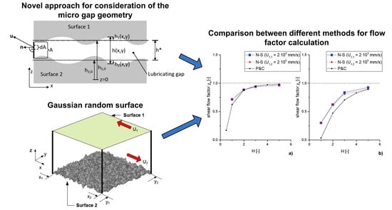
:The common approach for the flow factor calculation is based on using the Reynolds equation to simulate the micro-level flow. However, for structured surfaces the fluid flow cannot be represented correctly, due to the assumptions made when deriving the Reynolds equation. In this work, a novel method using the Navier-Stokes equations for the calculation of the micro-level flow is presented and validated against results from Patir and Cheng. The three-dimensional lubrication gap was generated by a rough Gaussian random surface and a perfectly smooth moving counter surface, in order to be available for different numerical methods. The presented results illustrate similar trends for both the approaches. Additionally, the use of the Navier-Stokes equations allows for the observance of surface induced effects which cannot be resolved by the approach of Patir and Cheng. Furthermore, a numerical approach for a shear flow factor calculation with a rough moving surface is presented and validated against other simulation methods. While the validation is maintained with pressure- and temperature-independent density and viscosity, these effects will be taken into account for later research activities of textured surfaces.
1. Introduction
In lubricated sliding contacts the separation of the two sliding surfaces is maintained by the internal fluid pressure of the lubricating film. In addition to the experimental investigation [1,2,3,4,5], the simulation of lubricated contacts is an important tool for the design process of tribological systems for different applications [6,7,8,9,10]. For the calculation of the hydrodynamic lubrication, the Reynolds equation is commonly used [11]. This equation is obtained from the Navier-Stokes equations under additional assumptions due to thin-film-flow in lubricated sliding contacts, e.g., journal bearings. Used in the classical sense, the Reynolds equation takes into account only the macroscopic geometry for calculating pressure distribution and friction losses. Hydrodynamic effects because of the microscopic surface structure are not taken into account. This is valid as long as the roughness of the surfaces is small in relation to the gap height. Especially in the case that the nominal gap height and the microstructural roughness are of the same order and partial lubrication occurs ( for Gaussian height distribution), the surface topography affects the fluid flow significantly, which needs to be considered in calculating hydrodynamic effects [12].
To take surface effects in fluid lubrication into account, two basic methods exist. For small contact areas, which generally occur in contra-form contacts (e.g., gear tooth contact,…), it is possible to directly incorporate measured microstructures in the hydrodynamic calculations, called direct coupling [13,14,15]. For conform contacts, also referred to as large-area contacts, however, this procedure is not yet effectively feasible since a direct incorporation of the surface topography results in enormous computational effort. In this case, a so-called indirect coupling is used. By calculating the fluid flow in a small representative area of the rough lubricating gap, the effects of the surface structures can be investigated on a reduced scale but with reasonable computational effort. By incorporating the achieved results in the form of flow factors in the Reynolds equation, the effects on the fluid flow resulting from the micro topography can be considered.
The now common method for indirect coupling goes back to Patir and Cheng [12,16]. The authors solved the Reynolds equation on a small area of the rough lubricating gap. The micro flow calculated in this way is set into relation to the flow of a perfectly smooth lubricating gap with the same mean height, resulting in flow factors. Fluid flow includes two possible sources, namely pressure and shear driven flow, which is also considered within the theory of flow factors by the introduction of pressure flow factors and shear flow factors.
The investigations by Patir and Cheng were conducted with mathematically generated surfaces, due to the lack of available real surface topographies. The basic assumption of surface height distribution is crucial. Besides the investigated case of a Gaussian height distribution by Patir and Cheng, the authors of [17] illustrated the effects of a different artificially generated surface which lead to deviant results. Nevertheless, flow factors from Patir and Cheng are the technical standard and also widely used in commercial simulation packages [18]. With advancing technology regarding the 3D acquisition of surfaces, the application of Patir and Cheng’s method became practicable for real surfaces [19,20,21]. In recent years, the method by Patir and Cheng has been adopted and expanded to be able to take effects like micro cavitation, elastic deformation, thermal effects and also solid contacts into account [22,23]. Lunde and Tonder [24] discuss the validity of the boundary conditions chosen by Patir and Cheng. The authors of [21,25] present new methods for micro-macro indirect coupling.
However, the use of the Reynolds equation for the calculation of the flow through the micro-structured lubricating gap is limited, due to the chosen simplifications. When the surface profile shows strong height changes, which can cause velocity changes in height direction, as well as changes of the fluid impulse and micro turbulences, the Reynolds equation is no longer valid to describe the flow through the rough gap [20,26,27,28,29,30]. Recent works describe the idea of calculating the micro flow and subsequently the flow factors with the Navier-Stokes equations and implementing them in a Reynolds equation for the large-scale system [31,32]. By using the Navier-Stokes equations, flow processes in the fluid can be depicted in greater detail. This is fundamental to being able to investigate the effects of structured and textured surfaces [33].
This article describes an approach for the calculation of flow factors using the Navier-Stokes equations. The presented method is designed for the use of a rough, three-dimensional lubrication gap. In contrast to mentioned references [31,32], which are subjected to the necessity of a smooth surface to be able to calculate the shear flow factor, the numerical approach is expanded by the possibility of a moving rough surface. With this novel method a deeper understanding of the effects of roughness and surface structures on the hydrodynamic lubricating performance is expected. The investigations in this article are performed with a mathematically generated surface in the theory presented by Patir and Cheng [12,16]. In this way, a comparison between the flow factors calculated by the Reynolds equation and the proposed method using the Navier-Stokes equations can be accomplished.
Since this is the first step in validating the described model, thermal effects, micro-cavitation and deformable geometry are not taken into account. Although they will increase computational effort considerably, these effects will be implemented in the future.
2. Mathematical Background
For the CFD simulation of the fluid flow in the rough lubrication gap, the Navier-Stokes equations [34] are used. Simplifying assumptions are constant viscosity ( mm/s) and absence of micro-cavitation. Because of the small dimensions of the gap, body forces are neglected. The equations are used in time-dependent, density-free formulation inside a three-dimensional domain with stationary reference frame. Moving surfaces, rough or smooth, act as fixed-velocity boundary conditions at the top and bottom of the computational domain. Pressure-induced elastic deformation is neglected, i.e., the bounding surfaces are rigid bodies moving at constant velocity with respect to the stationary frame. Consequently, the continuity equation can be written as
and the momentum equation as:
Boundary conditions for (2) at the inlet and outlet are the common ones, as used by Patir and Cheng [12,16], see in detail Section 3.2. To take micro turbulences into account, the flow simulation of the rough gap was obtained by a Large Eddy Simulation (LES) [35,36]. As width scale for the LES-filter a cube-root-volume-delta was used, where represents the volume of the respective cell of the numerical mesh [37].
As subgrid turbulence model, a one-equation-k-model was used [38].
The two sliding surfaces 1 and 2 exhibit local height changes and , which are measured from the mean level of each surface. Figure 1 is showing a 2D cross section through the 3D geometry with geometric definitions and visualization of the flow rate calculation. Pressure and velocity boundary conditions are described in Section 3.2. In the lubrication gap generated from these two surfaces, the nominal gap height , is defined as the difference between the mean levels of the two surfaces and :
The local rough gap height h is then defined as:
The solution of the Navier-Stokes equations for the rough lubrication gap results in a velocity and a pressure field. This data can be used to calculate the volume flow rate passing through a y-z cut plane with area A, located within the control volume. The volume flow rate of the rough gap is then defined as:
As described in [12,16], it is necessary to differentiate between pressure and shear driven effects. The implementation of appropriate boundary conditions (see Section 3.2) allows the calculation of the volume flow rate and subsequently the pressure and shear flow factors. In addition, a perfectly smooth lubricating gap shows a volume flow which can be defined by the Reynolds equation. The volume flow rate through an area with height and width b, driven by a pressure gradient is given by:
With respect to the relative velocity of the two sliding surfaces , the volume flow rate of a purely shear-driven flow can be formulated as follows:
The pressure and shear flow factors are calculated as ratios between the flow rates through a rough and a smooth gap of same nominal gap height given by Equations (9) and (10). This formulation is given by the publication of de Kraker [31,32].
Patir and Cheng [12,16] calculated flow factors for generic surfaces with normal-distributed roughness. For these surfaces, the authors defined empiric equations for the flow factors as a function of the normalized gap height H. In this paper these equations will be put in relation to the flow factor curves, calculated by the herein described method. By the use of the standard deviation of the rough surface, the normalized gap height H can be defined:
Besides the factor H, the orientation of the surface structure in relation to the flow direction also influences the flow factors. The orientation is given by the so-called Peklenik factor [39] which is the relation of the correlation lengths in x- and y-direction (at which the auto correlation function reduces to 50 percent of its original value). The suffixes subscripts x and y refer to directions along and perpendicular to the direction of flow.
A value of describes a roughness pattern of ridges and valleys oriented along the flow direction, while models surfaces with ridges and valleys perpendicular across the main flow direction. We will refer to these situation as “roughness oriented along or across flow direction” respectively.
The simulation results by Patir and Cheng were summarized with empiric fitting functions, varying between pressure and shear flow and orientation. With (11) and (12) the empiric equation for the pressure flow factor according to Patir and Cheng can be written as:
The empiric equation for the shear flow factor according to Patir and Cheng is given in a similar way (for the case in which the smooth surface is moving):
The constant fitting parameters in this equation for two orientations which we will investigate in this article are given in Table 1:
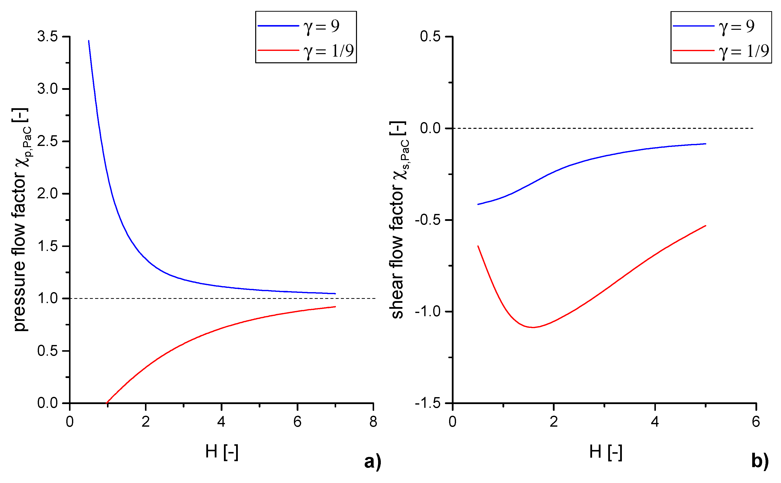
For visualization, the flow factors are plotted against H in Figure 2. Notice that for a pressure flow factor and for a shear flow factor the surface topography has no influence on the volume flow rate.
The empiric Equations (13) and (14) do not incorporate the influence of pressure and shear gradients. However, the non-linear terms of the Navier-Stokes equations allow the consideration of the effects of the pressure and shear gradient which shows significant effect on the fluid flow [31,32].
Implemented in the macro-scale Reynolds equation, the flow factors directly influence the behavior of tribological engineering elements, like journal bearings [40]. In this sense, structures which exhibit a lay cross the lubricant’s flow direction (), hampered the flow and showing a increased pressure build-up on the large scale system, but also a higher fluid friction. For cases where the surface structure is oriented along the flow direction (), an increasing flow compared to an ideal smooth gap can be recognized. This results in a reduced pressure build-up and, on the other hand, a lower fluid friction of the large scale system.
Literature review identifies different ways of implementating flow factors in the Reynolds equation. According to Patir and Cheng, the two-dimensional Reynolds equation with implemented flow factors is given by Equation (15) [12,16]. The flow factor is the pressure flow factor for a flow in y-direction and the surface velocities and are only applied in x-direction.
However, de Kraker suggests an implementation of the flow factors in the following way. The cross term factor, which considers the dependence between the pressure and the shear flow factor for strong structured surfaces, was not taken into account for the research in this article (see [32]):
To allow a comparison between the theory according to Patir and Cheng and the results obtained with the Navier-Stokes equations, both averaged Reynolds equations are equalized. For simplification, the -terms were neglected, like it would be in a contact with infinite width [41]. Furthermore, no overall cross flow in the computational domain and consequently, no extradiagonal flow factor terms occur because in our simulations the roughness structures are oriented strictly parallel or transverse to the main flow direction. In our case we use only one moving surface, so that we set .
For a purely pressure driven flow the surface velocity turn to zero and from Equation (17) only the pressure terms remain:
By solving this equation for it can be shown that the two pressure flow factors can be compared directly.
For a purely shear driven flow, no pressure gradient / is applied and Equation (17) turns into following form:
Integrating Equation (20) yields the following relation between and :
We use this relation to compare our approach to the Patir and Cheng method.
3. Numerical Method
3.1. Geometry and Mesh
For numerical simulation, the flow region was discretized by a hexahedral finite-volume mesh with around elements. While the top boundary was represented by a perfectly smooth plane, the bottom boundary was a surface created by applying a stationary Gaussian process with prescribed autocorrelation, standard deviation σ = 1 μm and mean (see Figure 3).
Gaussian height distribution is an assumption that does not necessarily hold for most types of tribological surfaces. However, the classical Patir and Cheng simulations [12] use Gaussian surfaces to calculate the flow factors. Furthermore, Tripp [42], deriving the flow factors analytically from a perturbation expansion of the pressure solution, calculates the flow factors for Gaussian surfaces. For the comparison between the results from Patir and Cheng and the Navier-Stokes flow simulation described here, the same statistical model for surface roughness was used. Specifically, we used an anisotropic autocorrelation function
with correlation lengths along the coordinate axes, so that the Peklenik factor measured the anisotropy.
In terms of grid resolution, the correlation lengths in our simulations were small multiples of the grid width. For the used Peklenik factors of 9 and 1/9 the lengths were chosen to be 1 node and 9 nodes. Even when other authors use longer correlation lengths [43,44], these values were chosen, based on the work of Patir and Cheng to achieve a proof of principle. As Tripp explains [42], the flow factors are not expected to be sensitive to the precise choice of correlation function, provided they refer to physically similar surface textures.
Realizations of random surfaces can be generated in various ways. Patir [12] generated them as moving averages of white-noise processes. For a discussion and generalization of this method see Bakolas [45]. Dietrich und Newsam [46] present an alternative method using circulant embedding and Fast Fourier Transform. Their technique has received increasing attention and implementations are readily available; see e.g., [47,48] and the references cited therein.
The x-y dimensions of the flow region were 200 μm × 200 μm. The nominal gap height was set to 5 μm, 3 μm, 2 μm and 1 μm to picture the trend of the flow factors over the gap height. The first contact between the surfaces took place between 2 μm and 3 μm. The solid contact regions were modeled as holes in the fluid mesh, which means that no flow occurred in contact areas.
3.2. Boundary Conditions
For the calculation of the pressure and the shear flow factor, different boundary conditions were implemented. For the pressure flow factor a pressure gradient
In flow direction was generated (see Table 2 and Figure 3). The boundaries at positions and were implemented as in- and outlet with given pressure. The fluid velocity vectors were variable to fulfill continuity. The boundaries at the positions and were created by the OpenFOAM -boundary “symmetry”, so that no flow through these faces were permitted and no shear forces were transferred. Surface 1 and 2 were implemented by the OpenFOAM-boundary “wall” (no flow through these faces and no slip-condition) and had no velocity.
For the shear flow simulation the pressure gradient was set to zero. Hence, the pressure at in- and outlet exhibited the same constant value and continuity-depended velocity. Depending on the case of interest either surface 1 or 2 was subjected to a velocity while the opposing surface remained at rest (see Table 3 and Figure 3). The other boundary conditions remained the same.
3.3. Numerical Schemes
The numerical simulation of the rough gap was carried out by the CFD-simulation tool “OpenFOAM”. The program is working with a Finite-Volume-Method. For the pressure correction, a SIMPLE-Algorithm was used. Within this algorithm the pressure gets corrected based on the continuity equation, using one iteration. The use of relaxation factors for holding the algorithm stable limit it to stationary problems. This makes it a stable and fast converging algorithm for stationary problems.
The stopping criterion for solving Equations (1) and (2) were a residual error for the velocity vector smaller than and for the pressure p smaller than . The relaxation factors for holding the SIMPLE-Algorithms stable, were set to .
For the calculation of the shear flow factor, measures concerning the realization of the boundary condition of the shearing surface needed to be applied. In the case of a moving smooth surface, the wall velocity was directly taken as boundary condition for the velocity field. This process is called “Mapping” in the following. When the rough surface introduces velocity, the application of a boundary velocity is no longer valid.
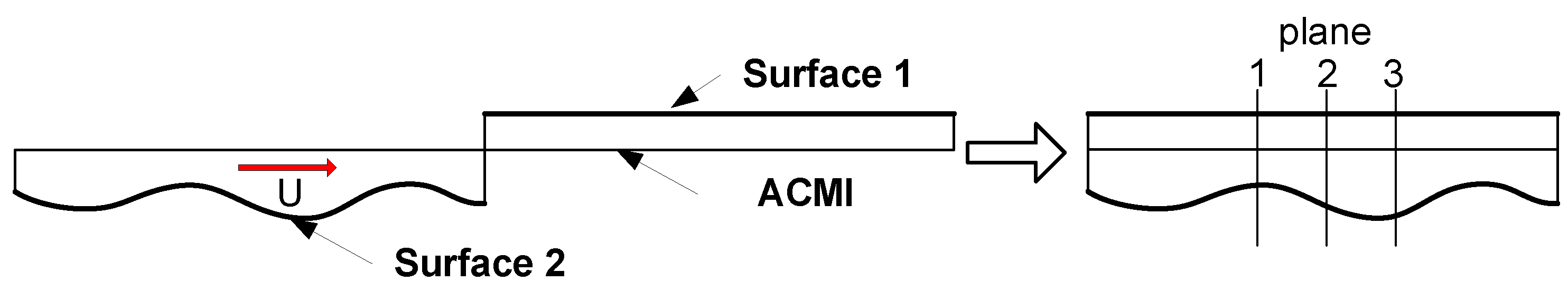
In this case the simulation was carried out by a “Moving Mesh”. The control volume was split in half so that each surface got assigned a fluid mesh (see Figure 4). Interaction between both mesh areas took place by using the OpenFOAM-boundary condition arbitrary coupled mesh interface (ACMI), which allows the interpolation of pressure and velocity data. The other boundary conditions were the same as described in Section 3.2.
For the shear flow simulation, both mesh areas were set into a starting position. A velocity U was applied in order to move the rough surface against the smooth until both completely overlap. Contrary to the previous case in which the use of a moving mesh represents an instationary process which consequently demands a PIMPLE-algorithm for the pressure correction. In contrast to the SIMPLE-Algorithm, several iterations for the pressure correction are used, so that no relaxation factors are needed. That is why this algorithm can also be used for instationary problems.
The time of solution varies between the method with stationary geometry with SIMPLE-Algorithms and moving mesh with PIMPLE-Algorithms between 3 to 4 h and several weeks. The calculations were carried out on 4 CPUs with Courant number-depending time step.
Because the moving mesh procedure requires a finite small volume between both boundaries, flow takes place at actual contact spots, see Figure 5. Hence, solid contact cannot be represented properly and the use of the “Moving Mesh” is only recommended in full fluid lubrication.
3.4. Post Processing
The volume flow rate passing through the rough gap is obtained by Equation (6), using the velocity field of the inlet boundary.
In case of the moving mesh, the volume flow rate is calculated at a separate cross-sectional plane. On this plane, meshed by triangles, the values of the pressure and velocity field are interpolated and used to calculate the volume flow rate by Equation (6). To get a representative flow rate for the computational domain, the averaged flow rate from three calculation planes is used, even when the differences in the flow rate were small between the different positions. Due to the relatively large structured area, three planes were considered sufficient to avoid numerical errors as well as influences from varying flow because of fluid transport in dimples. The planes are located at a distance of 10 μm to each other, with the central plane located in the center of the computational domain (see Figure 4).
4. Simulation Results and Discussion
For the described geometry pressure and shear flow factors for orientation, and were calculated and compared with the empirical equations of Patir and Cheng. To better understand the influence of the pressure and shear gradient as well as the difference between “Mapping” and “Moving Mesh” of the shear flow simulation, these matters were investigated.
4.1. Influence of Orientation and Pressure/Shear Gradient
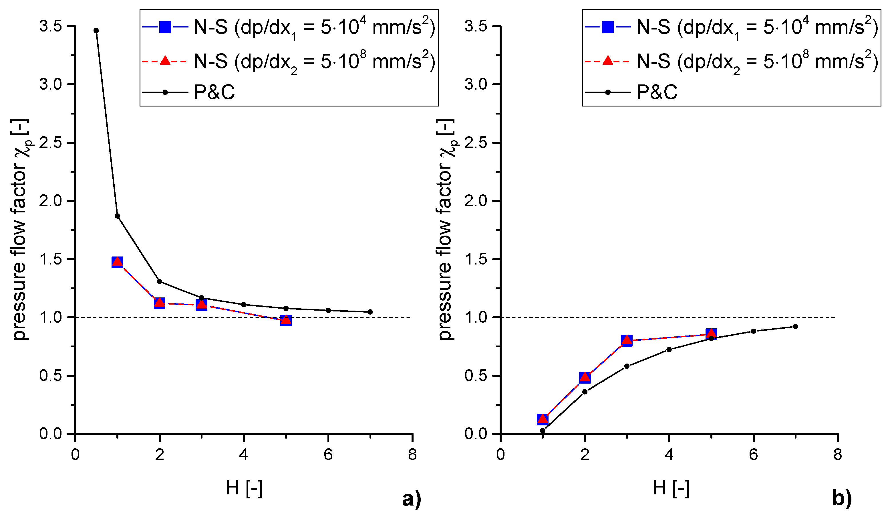
The pressure flow factors for the two different orientations can be directly compared with the curves according to Patir & Cheng. However, two different pressure gradients (density-free pressure (mm2/s2) is used), which represent operating conditions such as found those in lower and a higher loaded areas in a journal bearing, were applied (mm/s and mm/s). Every calculated data point in the following figures represents one CFD-simulation of the lubrication gap. Due to the computational effort, an averaging over several simulations was not used. Moreover, by using large surfaces which cover several multiples of the correlation length, averaging was not seen as necessary to achieve a proof of principle.
The results show the same trend as the curves according to Patir & Cheng (see Figure 6). When the surface structures are oriented along the flow direction, the flow factor is greater than 1, which means the volume flow in the rough lubricating gap is greater than in the perfectly smooth gap. It can be observed that the flow factor does not depend on the pressure gradient. This is due to the laminar flow regime (valid for the smaller and the larger pressure gradient) as well as the relatively smooth surface topography. A dependency on the pressure flow gradient may arise with stronger topography variation, like surface texturing [31,32]. Furthermore, the numerical simulation with the Navier-Stokes equations shows a more conservative behavior of the flow factors, which means that the roughness shows less influence on the flow behavior.
In the case of , which is for roughness pattern oriented across the main flow direction, numerical analysis with the Navier-Stokes equations, as well as the result from Patir & Cheng show a flow reduction, which lead to flow factors smaller than 1. In this case no influence of the pressure gradient could be recognized. Furthermore, the results from the Navier-Stokes simulation show a more conservative behavior. In addition, a characteristic kink at can be observed. This phenomenon could be related to the beginning contact of the two surfaces for -values between 2 and 3.
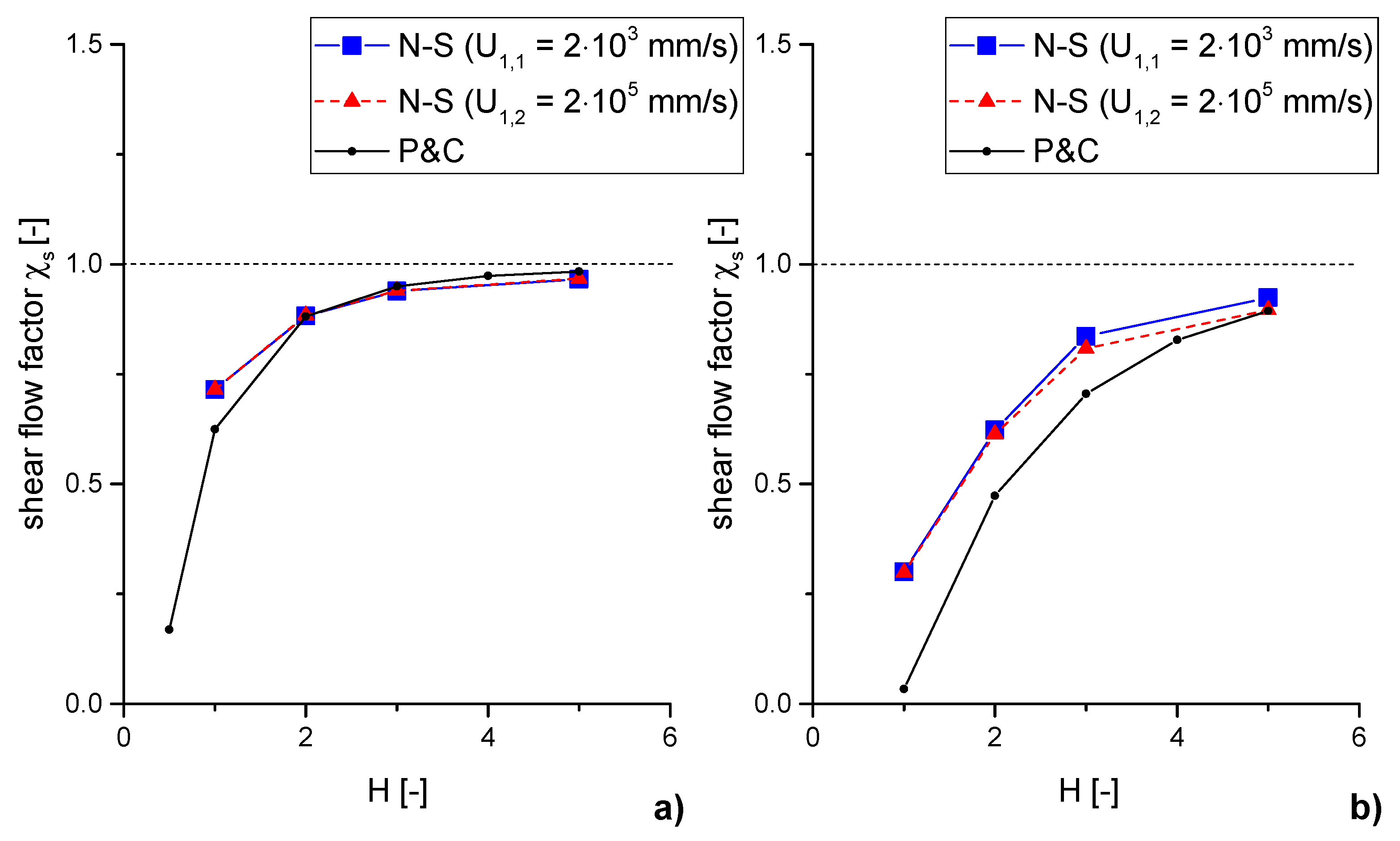
The shear flow factors (see Figure 7) were also calculated for two different relative velocities ( mm/s and mm/s). As moving surface the smooth one was chosen. The simulation was carried out by a “Mapping” of the wall velocity on the fluid velocity.
For the comparison of the calculated flow factors according to de Kraker and the flow factors by Patir and Cheng , the latter were converted, using Equation (21).
The results based on the Navier-Stokes equations show the same trends like the flow factors based on Patir & Cheng. For the roughness orientation in flow direction, the results from the Navier-Stokes equations show good agreement with the results of Patir and Cheng. For smaller gap heights Patir and Cheng predict a greater influence of the micro structure according to a smaller shear flow factor. The different relative velocities show no influence.
With roughness orientation across the flow direction, a larger difference results between the Patir and Cheng shear flow factors and the calculated ones. However, similar to the results of the pressure flow factor, the N-S curve shows a kink at . Furthermore, other authors recognize a poor fitting with their results to the results of Patir and Cheng for boundary conditions quite similar to those used in this paper [22,42,49].
Driven by different relative surface velocities, the results from the Navier-Stokes equations show differences at greater gap heights. This can by explained by the presence of micro-turbulences which are initiated from the cross-lying roughness structures. With rising gap height, the potential for turbulences rises, as it can be seen from the definition of the Reynolds number (see Equation (23)), which estimates the onset of turbulences.
4.2. Influence of the Numerical Method on the Shear Flow Factor
The difference between the numerical methods “Mapping”, “Moving Mesh” and the method according to Patir and Cheng were investigated. For a smooth moving wall both numerical methods are available. So the novel approach can be tested in contribution with other numerical methods. Because the use of a “Moving Mesh” needs a movable volume, a flow on contact points takes place. Due to this restriction for the use of the “Moving Mesh” at low gap heights, the contribution was performed at one gap height in full fluid friction regime. The results are given in the Table 4.
The difference between the different numerical methods is small and can by attributed to numerical errors. The method of Patir and Cheng shows a bigger difference because of the reasons described in the previous section (see Section 4.1). Thus, the moving mesh method is validated for simulation of shear flow caused by a moving rough surface. This task is performed in the next step.
For the same reasons that restrict the simulation of moving smooth surface, the simulation of the rough moving surface is carried out at full hydrodynamic lubrication. The results of the “Moving Mesh”-Simulation are compared with empiric equations from Patir and Cheng, for a rough moving surface. The results are given in the Table 5.
The results show the same trend as expected for a rough moving surface. The values are greater than 1 and indicate that the volume flow is greater than in a perfectly smooth gap. However, the accordance is good and the difference is not larger than in the previous investigations. This indicates a proper run of the shear flow simulation. Thus, by using a “Moving Mesh”, it is possible to investigate complex geometries also on the sliding surface.
5. Conclusions and Outlook
The results of Patir and Cheng for the calculation of flow factors [12,16] were compared with simulations based on Navier-Stokes equations for flow at the microscopic scale. The relatively soft height changes justify the use of the Reynolds equation. Nevertheless, the novel method using the mathematical approach of de Kraker [31,32] shows differences with the results from Patir and Cheng. This is attributed to the fact that just one surface was considered for calculation whereas Patir and Cheng performed an averaging of the results from 10 different surfaces.
Furthermore, the influence of pressure and shear gradient on the flow factors were investigated. For a laminar flow in the lubrication gap and the investigated geometry, the differences for the flow factors for different pressure and shear gradients are small or not present at all.
Moreover, the behavior of the shear flow factor for a moving rough surface was discussed. For this research, a numerical approach was designed which expands the method of de Kraker. After a validation of the novel method by the implementation of a smooth moving surface, the method was used to calculate the shear flow for a rough moving surface. However, due to restrictions for gap heights where solid contacts can occur, the method was only used for full fluid lubrication.
The goal for further works is to make the method also work for low gap heights, as well as to minimize the computation time. Especially, application to strongly structured surfaces will be the focus of further investigations. The research and development of textured surfaces for reducing friction or generating a faster pressure build-up in lubricating contacts, like journal bearings or linear sliders, are examples of the industrial use of the novel flow factor method.
Acknowledgments
Financial support by the Austrian Federal Government (in particular from Bundesministerium für Verkehr, Innovation und Technologie and Bundesministerium für Wissenschaft, Forschung und Wirtschaft) represented by Österreichische Forschungsförderungsgesellschaft mbH and the Styrian and the Tyrolean Provincial Government, represented by Steirische Wirtschaftsförderungsgesellschaft mbH and Standortagentur Tirol, within the framework of the COMET Funding Programme is gratefully acknowledged. Furthermore, we would like to thanks our colleagues, Alexander Vakhrushev and Tobias Holzmann from the Chair of Simulation and Modeling Metallurgical Processes, for the technical support with the CFD tool “OpenFOAM”.
Author Contributions
Michael Pusterhofer and Philipp Bergmann were setting up the method and writing the article, the simulations were carried out by Michael Pusterhofer. Clemens Brand generated the Gaussian random surface and wrote the section “Geometry and Mesh”. Florian Summer and Florian Grün took over consulting tasks and advisory activities.
Conflicts of Interest
The authors declare no conflict of interest.
Nomenclature
| Variable | Name |
| velocity vector | |
| ∇ | Nabla operator |
| t | time |
| p | fluid pressure |
| fluid density | |
| kinematic viscosity | |
| normal vector | |
| b | width of the control volume |
| Q | volume flow rate |
| pressure flow factor | |
| shear flow factor | |
| H | non-dimensional height factor () |
| Peklenik (orientation) factor () | |
| correlation length | |
| relative velocity | |
| standard deviation of the combined surface profile | |
| coordinates of the three-dimensional space | |
| h | local gap height |
| nominal gap height | |
| height changes of one surface measured from its mean level |
References
- Ramesh, A.; Akram, W.; Mishra, S.P.; Cannon, A.H.; Polycarpou, A.A.; King, W.P. Friction characteristics of microtexured surfaces under mixed and hydrodynamic lubrication. Tribol. Int. 2013, 57, 170–176. [Google Scholar] [CrossRef]
- Grün, F.; Gódor, I.; Gärtner, W.; Eichlseder, W. Tribological performance of thin overlays for journal bearings. Tribol. Int. 2011, 44, 1271–1280. [Google Scholar] [CrossRef]
- Summer, F.; Grün, F.; Schiffer, J.; Gódor, I.; Papadimitriou, I. Tribological study of crankshaft bearing systems: Comparison of forged steel and cast iron counterparts under start-stop operation. Wear 2015, 338–339, 232–241. [Google Scholar] [CrossRef]
- Bergmann, P.; Grün, F.; Summer, F.; Gódor, I.; Stadler, G. Expansion of the metrological visualization capability by the implementation of acoustic emission analysis. Adv. Tribol. 2017, 2017. [Google Scholar] [CrossRef]
- Moder, J.; Grün, F.; Stoschka, M.; Gódor, I. A Novel Two-Disc Machine for High Precision Friction Assessment. Adv. Tribol. 2017, 2017. [Google Scholar] [CrossRef]
- Chunxing, G.; Xianghui, M.; Youbai, X.; Di, Z. Mixed lubrication problems in the presence of textures: An efficient solution to the cavitation problem with consideration of roughness effects. Tribol. Int. 2016, 103, 516–528. [Google Scholar]
- Quinonez, A.F.; Morales-Espejel, G.E. Surface roughness effects in hydrodynamic bearings. Tribol. Int. 2016, 98, 212–219. [Google Scholar] [CrossRef]
- Ruggiero, A.; Gomez, E.; D’Amato, R. Approximate Analytical Model for the Speeze-Film Lubrication of the Human Ankle Joint with Synovial Fluid Filtrated by Articular Cartilage. Tribol. Lett. 2011, 41, 337–343. [Google Scholar] [CrossRef] [Green Version]
- Ruggiero, A.; Gomez, E.; D’Amato, R. Approximate closed-form solution of the synovial fluid film force in the human ankle joint with non-Newtonian lubricant. Tribol. Int. 2013, 57, 156–161. [Google Scholar] [CrossRef]
- D’Amato, R.; Calvo, R.; Gomez, E. Sensitivity study of the morphometric fitting on the pressure field inside ankle joints. Case Stud. Mech. Syst. Signal Process. 2015, 1, 8–14. [Google Scholar] [CrossRef]
- Reynolds, O. On the Theory of Lubrication and its Application to Mr. Beauchamp Tower’s Experiments, including an Experimental Determination of the Viscosity of Olive Oil. Philos. Trans. R. Soc. Lond. 1886, 177, 157–234. [Google Scholar] [CrossRef]
- Patir, N.; Cheng, H.S. An average flow model for determining effects of three-dimensional roughness on partial hydrodynamic lubrication. J. Lubr. Technol. 1978, 100, 12–17. [Google Scholar] [CrossRef]
- Xu, G.; Sadeghi, F. Thermal EHL analysis of circular contacts with measured surface roughness. J. Tribol. 1989, 118, 473–482. [Google Scholar] [CrossRef]
- Chang, L.; Farnum, C. A thermal model for elastohydrodynamic lubrication of rough surfaces. Tribol. Trans. 1992, 35, 281–286. [Google Scholar] [CrossRef]
- Dobrica, M.B.; Fillon, M.; Maspeyrot, P. Influence of mixed-lubrication and rough elastic-plastic contact on the performance of small fluid film bearings. Tribol. Trans. 2008, 51, 699–717. [Google Scholar] [CrossRef]
- Patir, N.; Cheng, H.S. Application of average flow model to lubrication between rough sliding surfaces. J. Lubr. Technol. 1979, 101, 220–230. [Google Scholar] [CrossRef]
- Wilson, W.R.D.; Marsault, N. Partial hydrodynamic lubrication with large fractional contact areas. J. Tribol. 1998, 120, 16–20. [Google Scholar] [CrossRef]
- Offner, G.; Knaus, O. A Generic Friction Model for Radial Slider Bearing Simulation Considering Elastic and Plastic Deformation. Lubricants 2015, 3, 522–538. [Google Scholar] [CrossRef]
- Knoll, G. Elastohydrodynamische Simulationstechnik mit integriertem Mischreibungskontkat. Materialwissenschaft und Werkstofftechnik 2003, 34, 946–952. [Google Scholar] [CrossRef]
- Brenner, G.; Al-Zoubi, A.; Mukinovic, M.; Schwarze, H.; Swoboda, S. Numerical simulation of surface roughness effects in laminar lubrication using the Lattice-Boltzmann Method. J. Tribol. 2007, 129, 603–610. [Google Scholar] [CrossRef]
- Sahlin, F.; Almqvist, A.; Larsson, R.; Glavatskih, S.B. Rough surface flow factors in full film lubrication based on a homogenization technique. Tribol. Int. 2007, 40, 1025–1034. [Google Scholar] [CrossRef]
- Meng, F.M.; Cen, S.Q.; Hu, Y.Z.; Wang, H. On elastic deformation, inter-asperity cavitation and lubricant thermal effects on flow factors. Tribol. Int. 2009, 42, 260–274. [Google Scholar] [CrossRef]
- Chengwei, W.; Linqing, Z. An average Reynold Equation for partial film lubrication with a contact factor. J. Tribol. 1989, 111, 188–191. [Google Scholar]
- Lunde, L.; Tonder, K. Pressure and shear flow in a rough hydrodynamic bearing, flow factor calculation. J. Tribol. 1997, 119, 549–555. [Google Scholar] [CrossRef]
- Almqvist, A.; Fabricius, J.; Spencer, A.; Wall, P. Similarities and differences between the flow factor method by Patir and Cheng and homogenization. J. Tribol. 2011, 133. [Google Scholar] [CrossRef]
- Sahlin, F.; Glavatskih, S.B.; Almqvist, T.; Larsson, R. Two-dimensional CFD-Analysis of micro-patterned surfaces in hydrodynamic lubrication. J. Lubr. Technol. 2005, 127, 96–102. [Google Scholar] [CrossRef]
- Brajdic-Mitidieri, P.; Gosman, A.D.; Ioannides, E.; Spikes, H.A. CFD analysis of a low friction pocketed pad bearing. J. Tribol. 2005, 127, 803–812. [Google Scholar] [CrossRef]
- Arghir, M.; Roucou, N.; Helene, M.; Frene, J. Theoretical analysis of the incompressible laminar flow in a macro-roughness cell. J. Tribol. 2003, 125, 309–318. [Google Scholar] [CrossRef]
- Dobrica, M.B.; Fillon, M. About the validity of Reynolds equation and inerta effects in textured sliders of infinite width. Proc. Inst. Mech. Eng. Part J J. Eng. Tribol. 2009, 223, 69–78. [Google Scholar] [CrossRef]
- Bayada, G.; Chambat, M. New Models in the Theory of the Hydrodynamic Lubrication of Rough Surfaces. J. Tribol. 1988, 110, 402–407. [Google Scholar] [CrossRef]
- De Kraker, A.; van Ostayen, R.A.J.; Rixen, D.J. A Multiscale Method Modeling Surface Texture Effects. J. Tribol. 2006, 129, 221–230. [Google Scholar] [CrossRef]
- De Kraker, A.; van Ostayen, R.A.J.; Rixen, D.J. Development of a texture averaged Reynolds equation. Tribol. Int. 2010, 43, 2100–2109. [Google Scholar] [CrossRef]
- Yildiran, I.N.; Temizer, I.; Cetin, B. Homogenization in Hydrodynamic Lubrication: Microscopic Regimes and Re-Entrant Textures. J. Tribol. 2017, 140. [Google Scholar] [CrossRef]
- Bestehorn, M. Hydrodynamik und Strukturbildung; Springer: Berlin/Heidelberg, Germany, 2006. [Google Scholar]
- Fröhlich, J. Large Eddy Simulation Turbuleter Strömungen; Teubner Verlag: Wiesbaden, Germany, 2006. [Google Scholar]
- Lesieur, M.; Metais, O.; Comte, P. Large-Eddy Simulations of Turbulence; Cambridge University Press: Cambridge, UK, 2005. [Google Scholar]
- Deardorff, J.W. The use of subgrid transport equations in a three-dimensional model of athmospheric turbulence. J. Fluids Eng. 1973, 95, 429–438. [Google Scholar] [CrossRef]
- Yoshizawa, A. Statistical theory for compressible turbulent shear flows, with the application to subgrid modeling. Phys. Fluids 1986, 29, 2152–2164. [Google Scholar] [CrossRef]
- Peklenik, J. New Developments in Surface Characterization and Measurement by Means of Random Process Analysis. Proc. Inst. Mech. Eng. 1967, 182, 108–126. [Google Scholar] [CrossRef]
- Knoll, G.; Boucke, A.; Winijsart, A.; Stapelmann, A.; Auerbach, P. Reduction of Friction Losses in Journal Bearings of Valve Train Shaft by Application of Running-in Profile. Tribologie und Schmierungstechnik 2016, 63, 14–21. [Google Scholar]
- Vogelpohl, G. Betriebssichere Gleitlager; Springer: Berlin/Heidelberg, Germany; New York, NY, USA, 1967. [Google Scholar]
- Tripp, J.H. Surface roughness effects in hydrodynamic lubrication: The flow factor method. J. Lubr. Technol. 1983, 105, 458–463. [Google Scholar] [CrossRef]
- Harp, S.; Salant, R. An Average Flow Model of Rough Surface Lubrication with Inter-Asperity Cavitation. J. Tribol. 2001, 123, 134–143. [Google Scholar] [CrossRef]
- Peeken, H.; Knoll, G.; Rienäcker, A.; Lang, J.; Schönen, R. On the Numerical Determination of Flow Factors. J. Tribol. 1997, 119, 259–264. [Google Scholar] [CrossRef]
- Bakolas, V. Numerical generation of arbitrarily oriented non-gaussian three-dimensional rough surfaces. Wear 2003, 254, 546–554. [Google Scholar] [CrossRef]
- Dietrich, C.R.; Newsam, G.N. Fast and exact simulation of stationary gaussian processes through circulant embedding of the covariance matrix. SIAM J. Sci. Comput. 1997, 18, 1088–1107. [Google Scholar] [CrossRef]
- Sykulski, A.M.; Percival, D.B. Exact simulation of noncircular or improper complex-valued stationary Gaussian processes using circulant embedding. In Proceedings of the IEEE 26th International Workshop on Machine Learning for Signal Processing, Salerno, Italy, 13–16 September 2016; pp. 1–6. [Google Scholar]
- Kroese, D.P.; Botev, Z.I. Spatial Process Generation. arXiv, 2013; arXiv:1308.0399. [Google Scholar]
- Elrod, H.G. A general theory for laminar lubrication with Reynolds roughness. J. Tribol. 1979, 101, 8–14. [Google Scholar] [CrossRef]
Figure 1.
Definition of the fluid film gap geometry and the flow rate calculation.
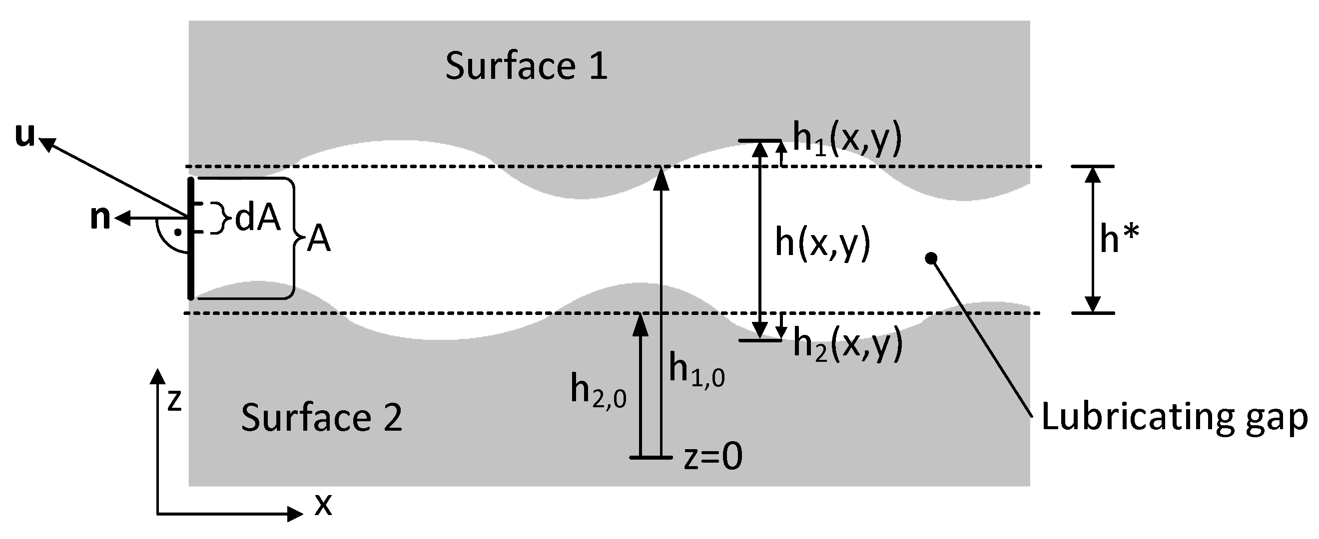
Figure 2.
Flow factors calculated by Patir & Cheng for two different ( means roughness orientation is parallel to the flow direction, means roughness orientation is cross the flow direction) [12,16]: (a) Pressure flow factor (b) Shear flow factor for a moving smooth surface and stationary rough surface.

Figure 3.
Control volume for the numerical simulation.
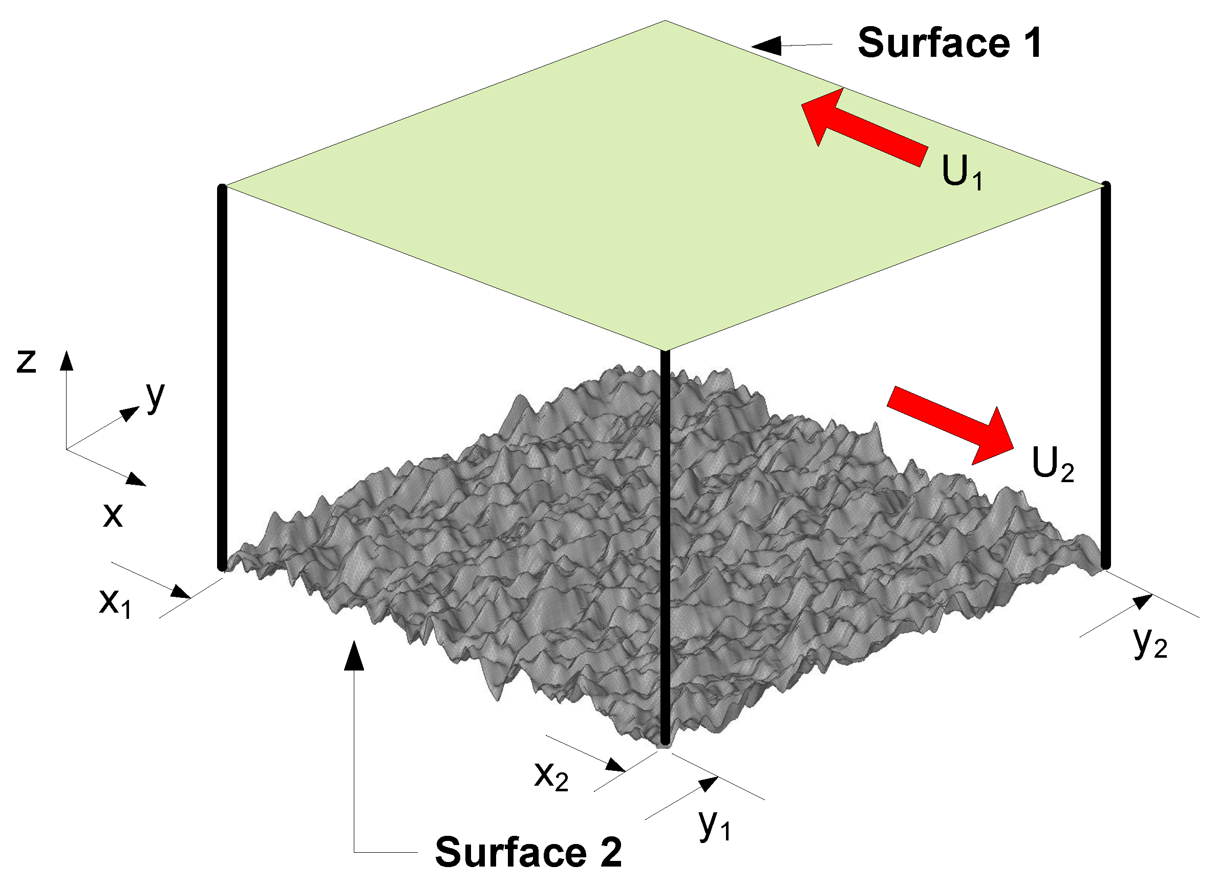
Figure 4.
Procedure of the simulation with a “Moving Mesh” and position of the calculation planes.

Figure 5.
Simulation with a “Moving Mesh” for variable gap height.
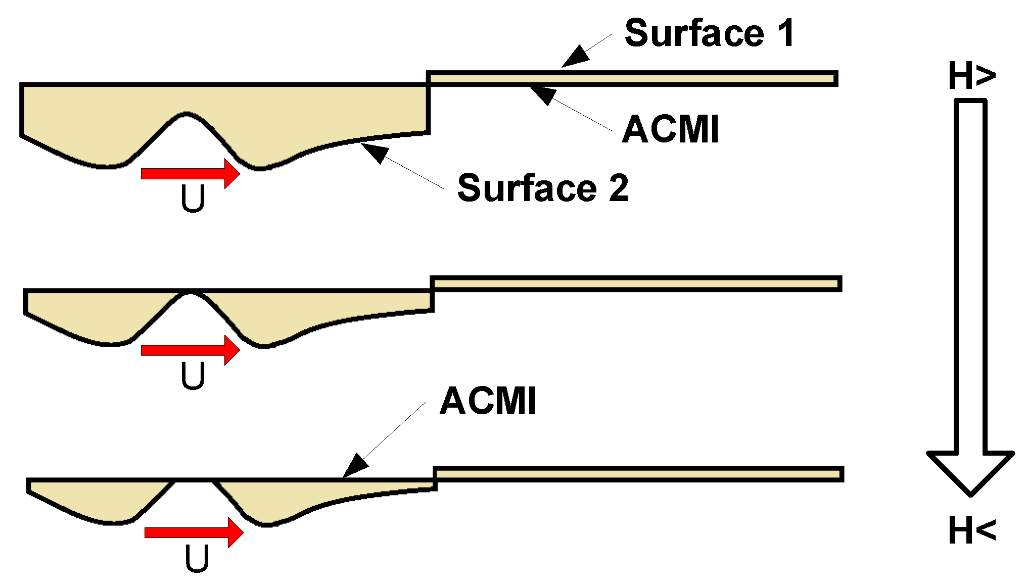
Figure 6.
Pressure flow factors calculated by the Navier-Stokes equations (N-S) for two different pressure gradients compared with the factors calculated by Patir & Cheng (P&C): (a) Roughness orientation in flow direction (); (b) Roughness orientation cross the flow direction ().
Figure 6.
Pressure flow factors calculated by the Navier-Stokes equations (N-S) for two different pressure gradients compared with the factors calculated by Patir & Cheng (P&C): (a) Roughness orientation in flow direction (); (b) Roughness orientation cross the flow direction ().

Figure 7.
Shear flow factors for a smooth moving surface calculated by the Navier-Stokes equations (N-S) for two different velocities compared with the factors calculated by Patir & Cheng (P&C): (a) Roughness orientation in flow direction (); (b) Roughness orientation cross the flow direction ().
Figure 7.
Shear flow factors for a smooth moving surface calculated by the Navier-Stokes equations (N-S) for two different velocities compared with the factors calculated by Patir & Cheng (P&C): (a) Roughness orientation in flow direction (); (b) Roughness orientation cross the flow direction ().

| C | r | |||||
|---|---|---|---|---|---|---|
| 1/9 | 1.48 | 0.42 | 2.046 | 1.12 | 0.78 | 0.03 |
| 9 | 0.87 | 1.5 | 1.011 | 0.54 | 1.07 | 0.08 |
Table 2.
Boundary conditions for the calculation of the pressure flow factor [12].
Table 2.
Boundary conditions for the calculation of the pressure flow factor [12].
| Position | Boundary Condition |
|---|---|
| Surface 1 | |
| Surface 2 |
Table 3.
Boundary conditions for the calculation of the shear flow factor [16].
Table 3.
Boundary conditions for the calculation of the shear flow factor [16].
| Position | Boundary Condition |
|---|---|
| Surface 1 | |
| Surface 2 |
Table 4.
Comparison between flow factors according to Patir and Cheng and flow factors calculated by “Mapping” and “Moving Mesh” for a smooth moving surface.
Table 4.
Comparison between flow factors according to Patir and Cheng and flow factors calculated by “Mapping” and “Moving Mesh” for a smooth moving surface.
| Patir & Cheng | Mapping | Moving Mesh | |
|---|---|---|---|
| Normalized gap height H (-) | 5.2 | 5.2 | 5.2 |
| Orientation (-) | 9 | 9 | 9 |
| Surface velocity (mm/s) | |||
| Shear flow factor (-) | 0.984 | 0.968 | 0.967 |
Table 5.
Comparison between flow factors calculated by “Moving Mesh” and the method according to Patir and Cheng for a rough moving surface.
Table 5.
Comparison between flow factors calculated by “Moving Mesh” and the method according to Patir and Cheng for a rough moving surface.
| Patir & Cheng | Moving Mesh | |
|---|---|---|
| Normalized gap height H (-) | 5.2 | 5.2 |
| Orientation (-) | 9 | 9 |
| Surface velocity (mm/s) | ||
| Shear flow factor (-) | 1.097 | 1.086 |
© 2018 by the authors. Licensee MDPI, Basel, Switzerland. This article is an open access article distributed under the terms and conditions of the Creative Commons Attribution (CC BY) license (http://creativecommons.org/licenses/by/4.0/).
Share and Cite
MDPI and ACS Style
Pusterhofer, M.; Bergmann, P.; Summer, F.; Grün, F.; Brand, C. A Novel Approach for Modeling Surface Effects in Hydrodynamic Lubrication. Lubricants 2018, 6, 27. https://doi.org/10.3390/lubricants6010027
AMA Style
Pusterhofer M, Bergmann P, Summer F, Grün F, Brand C. A Novel Approach for Modeling Surface Effects in Hydrodynamic Lubrication. Lubricants. 2018; 6(1):27. https://doi.org/10.3390/lubricants6010027
Chicago/Turabian StylePusterhofer, Michael, Philipp Bergmann, Florian Summer, Florian Grün, and Clemens Brand. 2018. "A Novel Approach for Modeling Surface Effects in Hydrodynamic Lubrication" Lubricants 6, no. 1: 27. https://doi.org/10.3390/lubricants6010027
Note that from the first issue of 2016, this journal uses article numbers instead of page numbers. See further details here.