Evaluation of Wear Phenomena of Journal Bearings by Close to Component Testing and Application of a Numerical Wear Assessment


Abstract
:1. Introduction
2. Materials and Methods
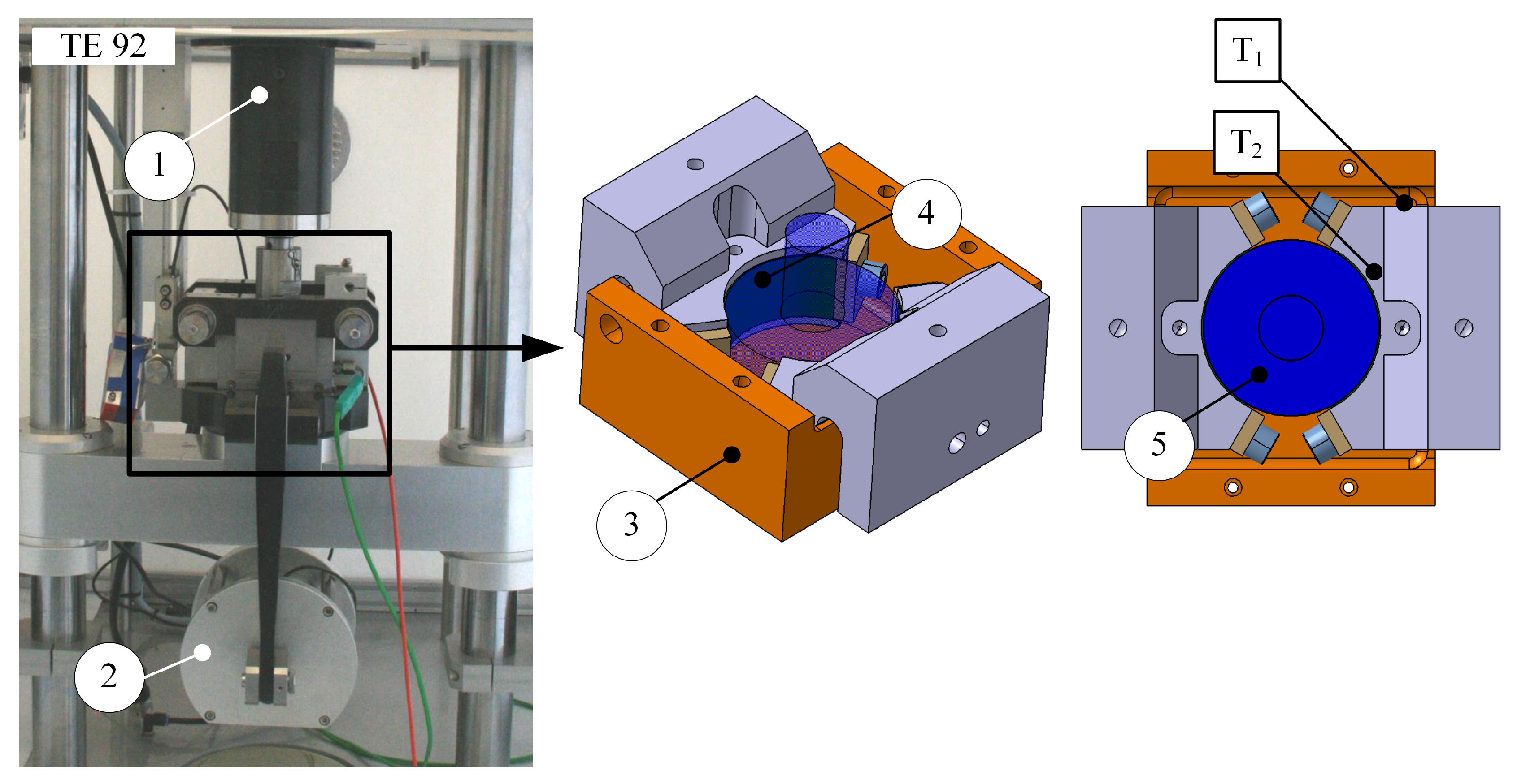
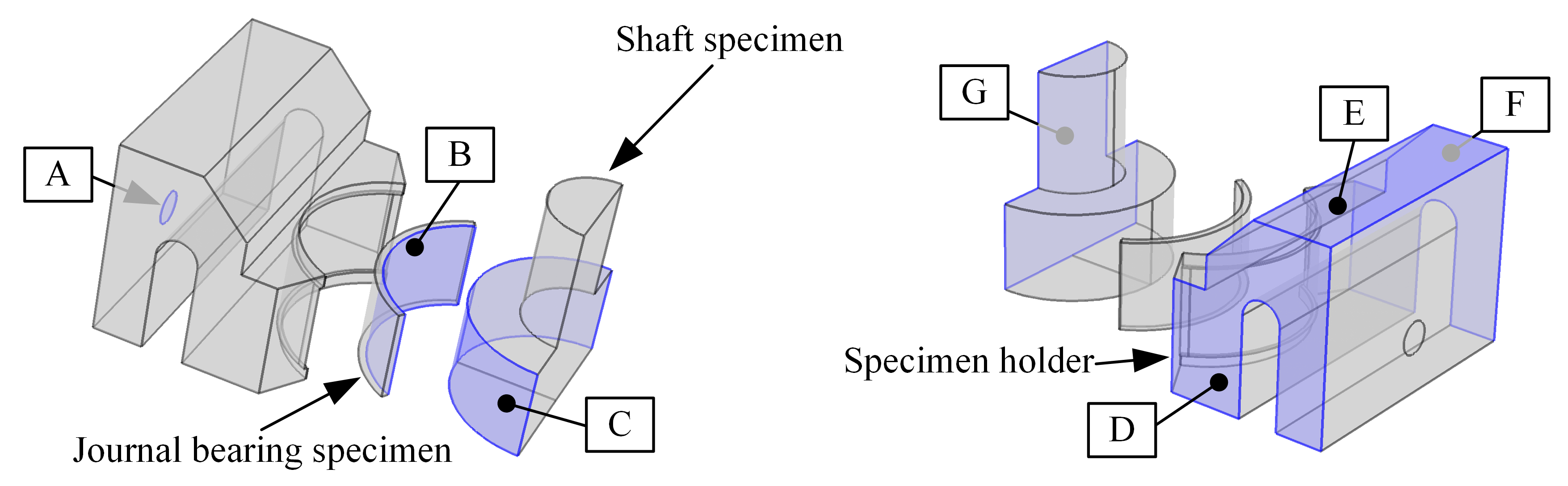
2.1. Test Setting
2.2. Test Strategies
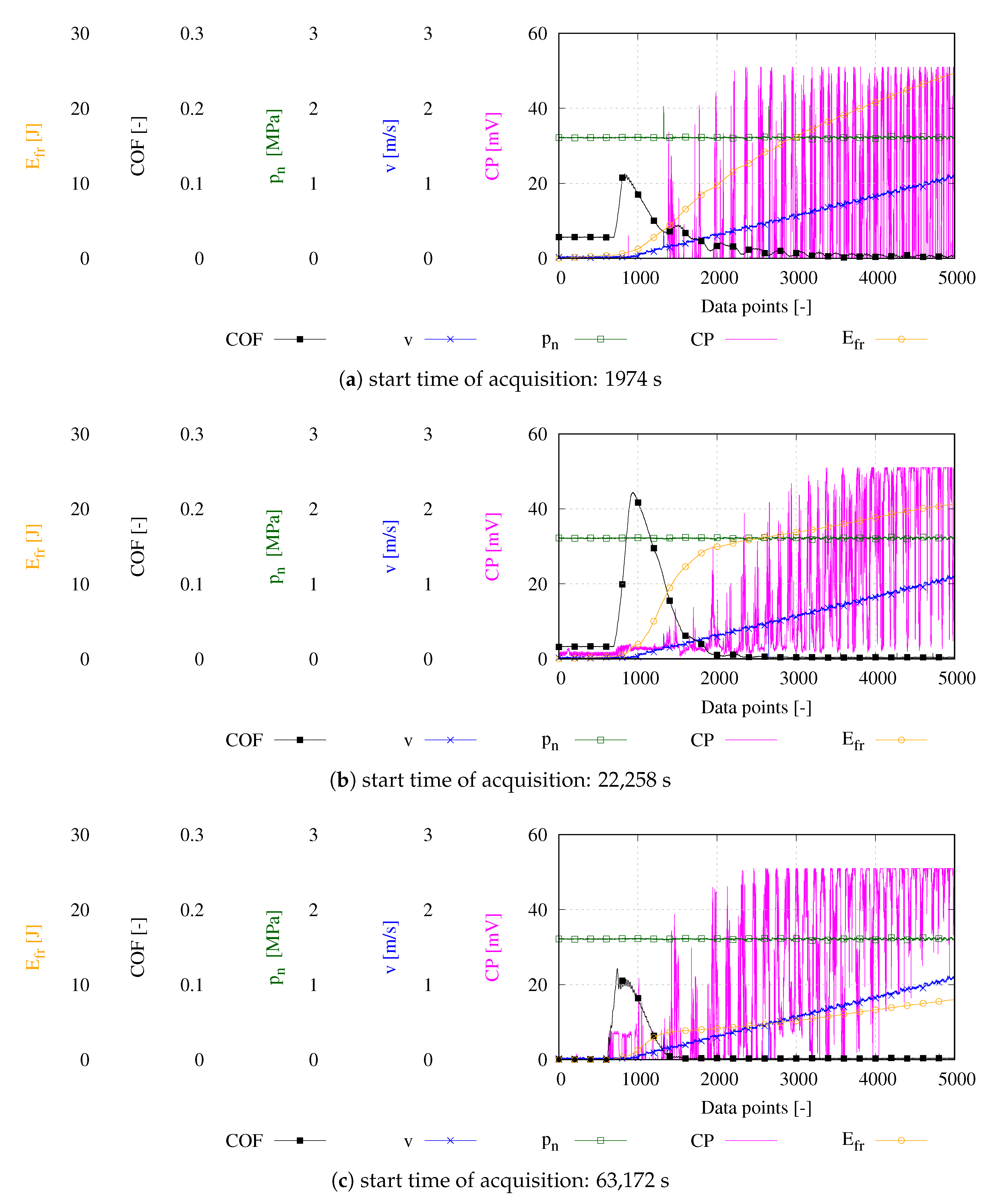
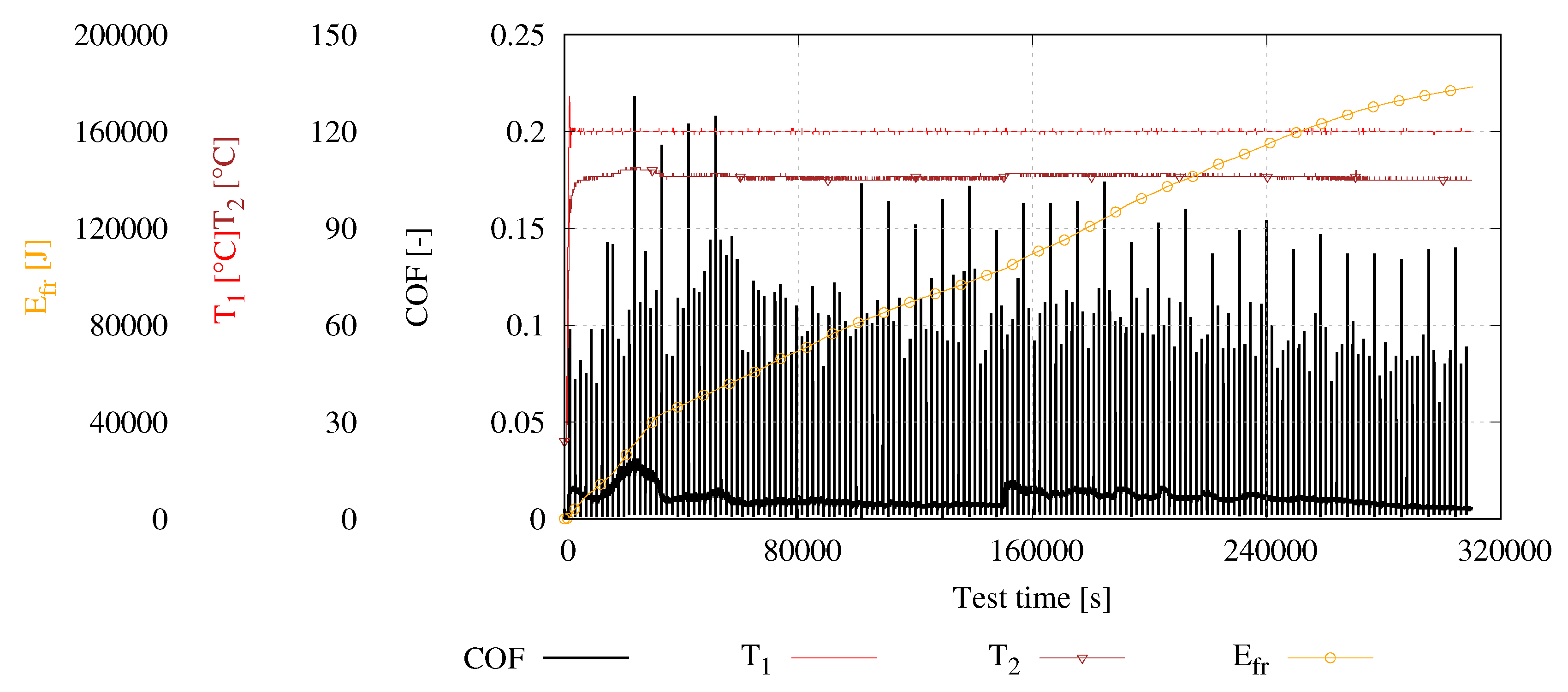
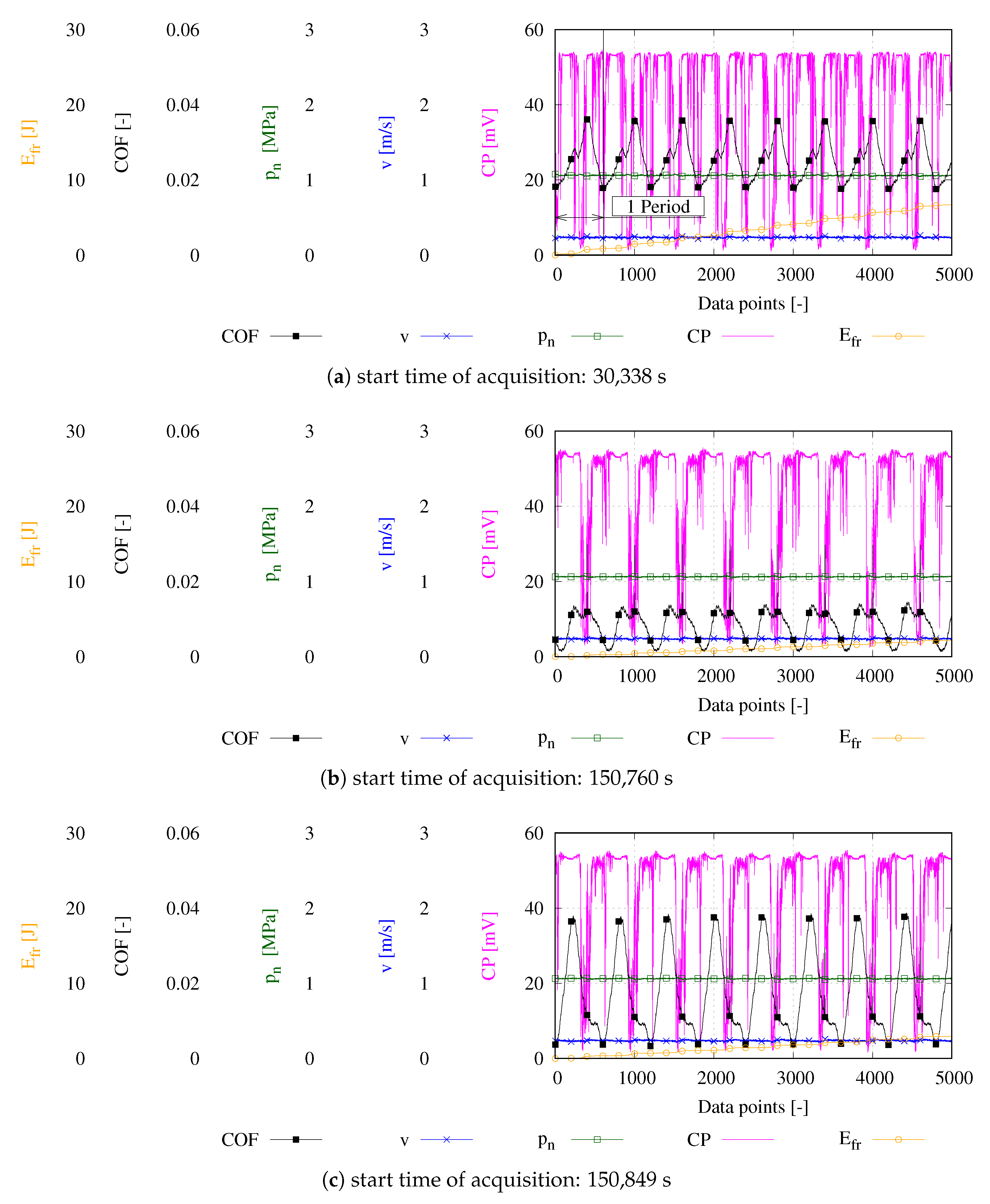
2.3. Test Evaluation
2.4. Test Materials
2.5. Simulation
2.5.1. Governing Equations
2.5.2. Model Description
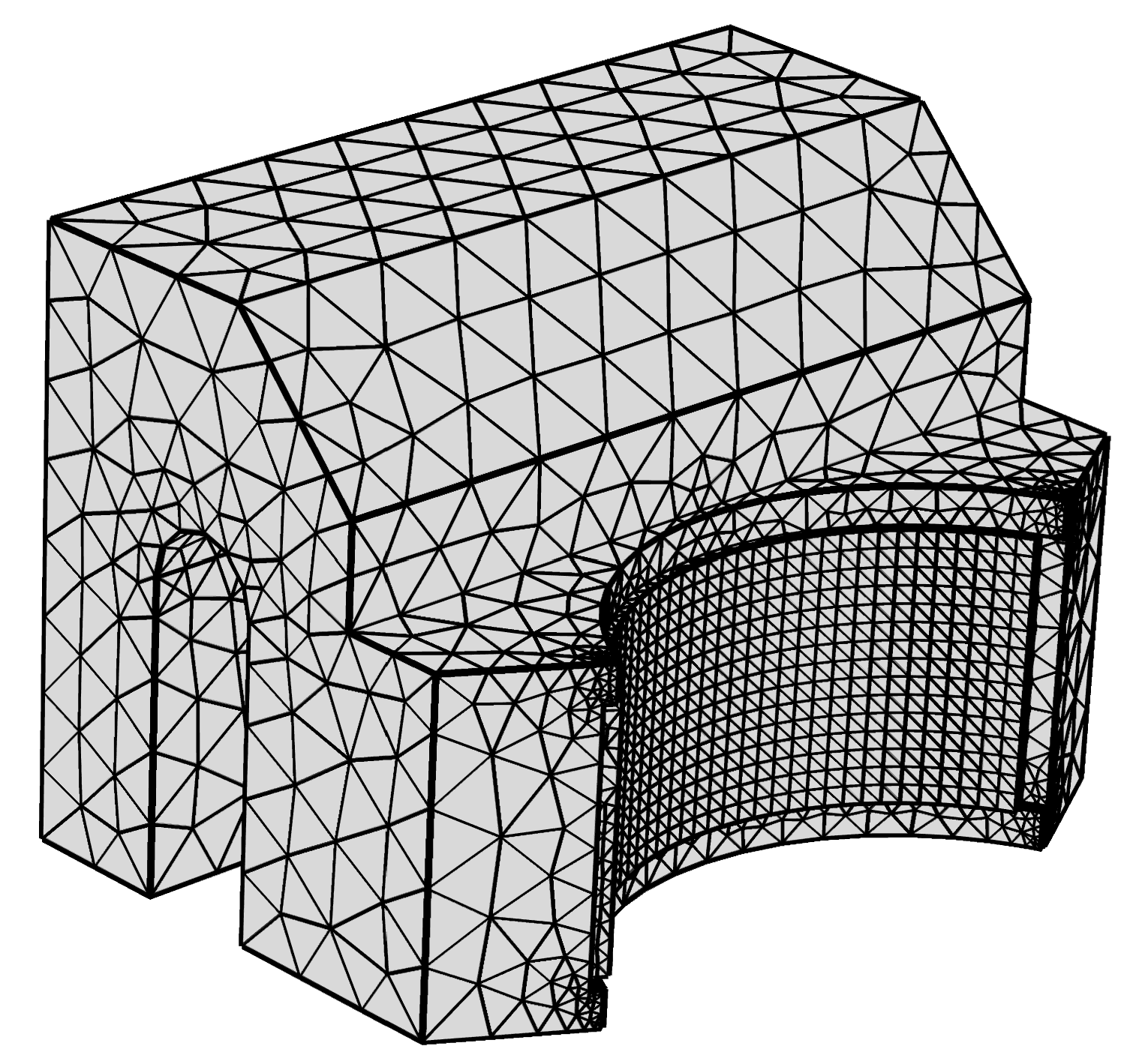
2.5.3. Mesh
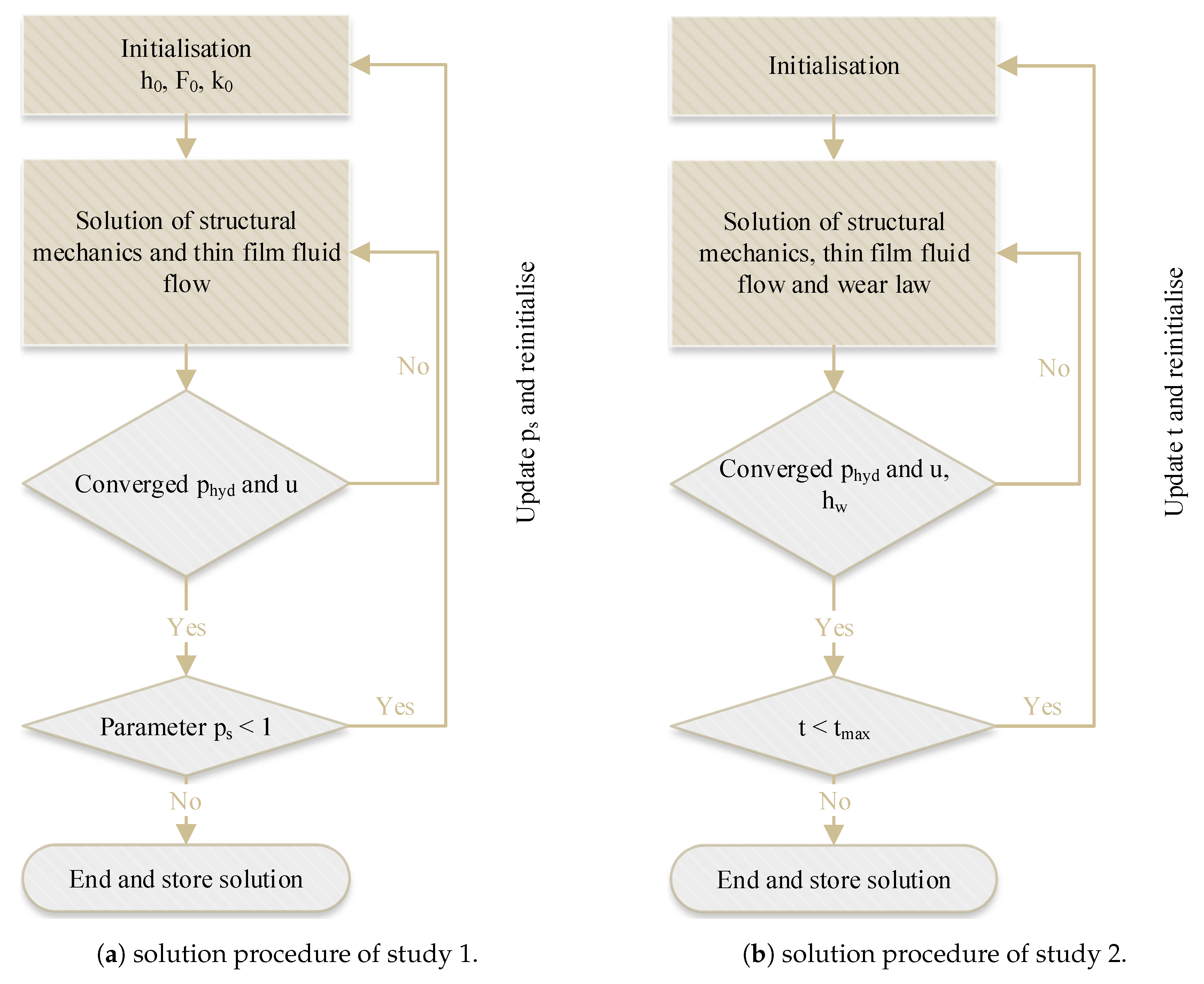
2.5.4. Numerical Procedure
3. Results and Discussion
3.1. Tribological Results
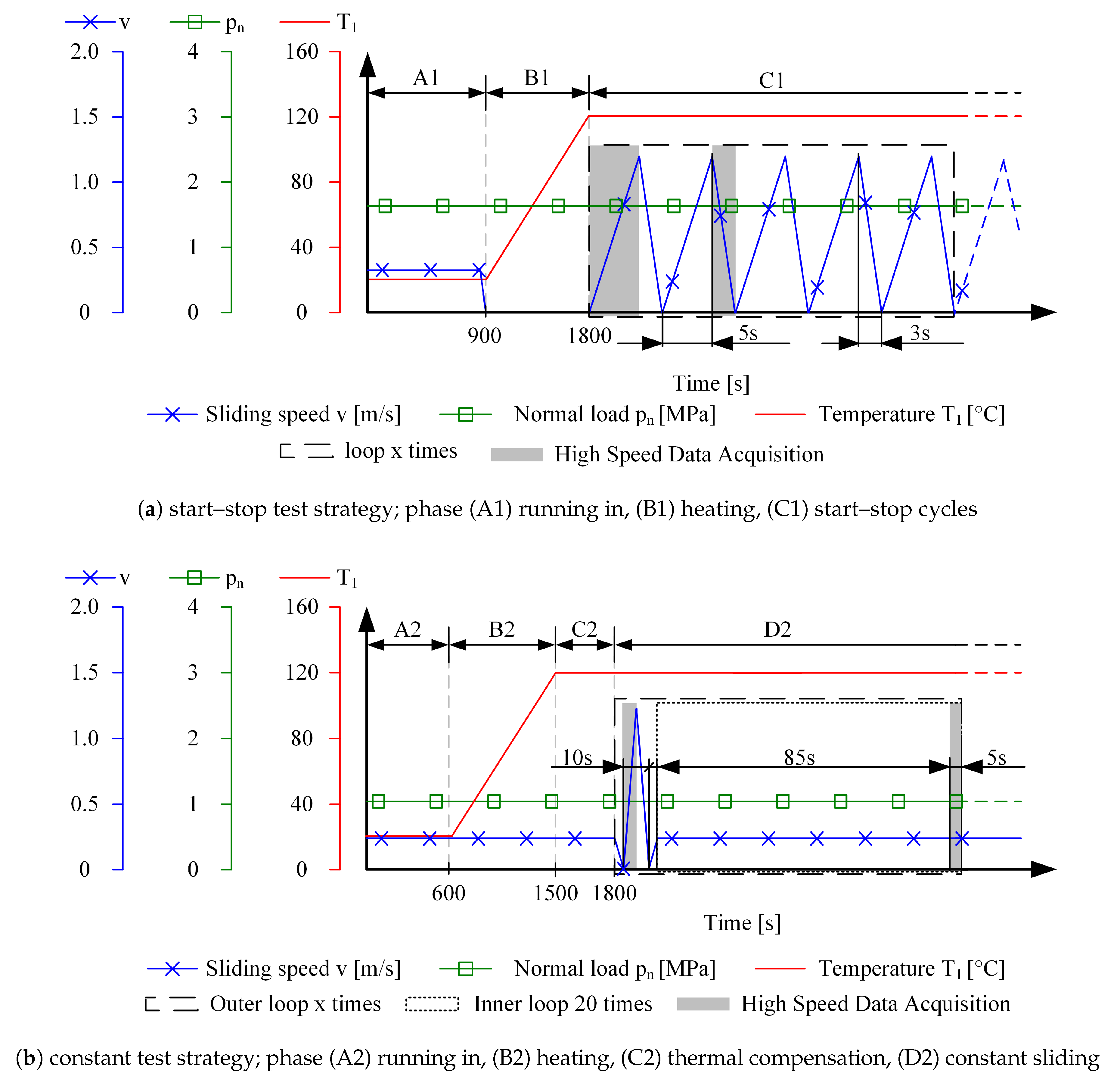
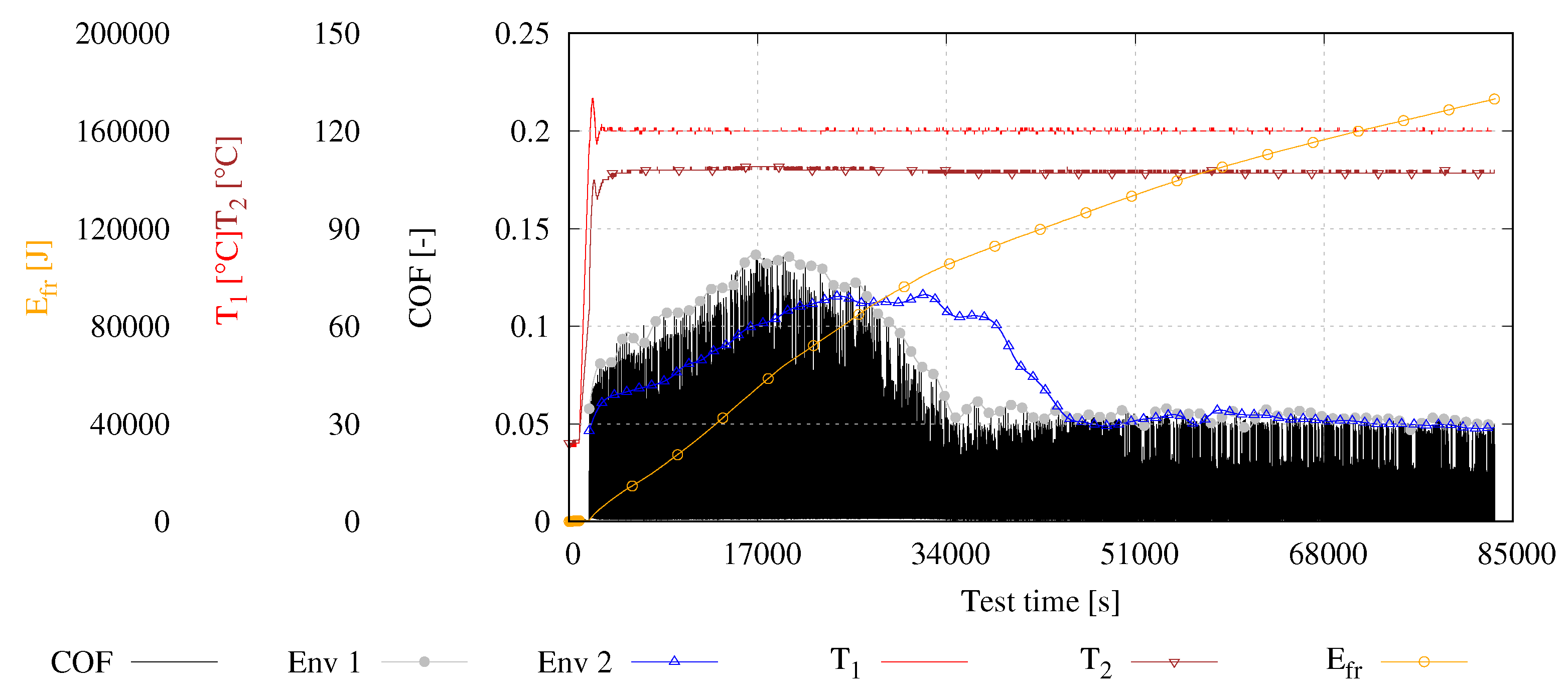
3.1.1. Start–Stop
3.1.2. Constant
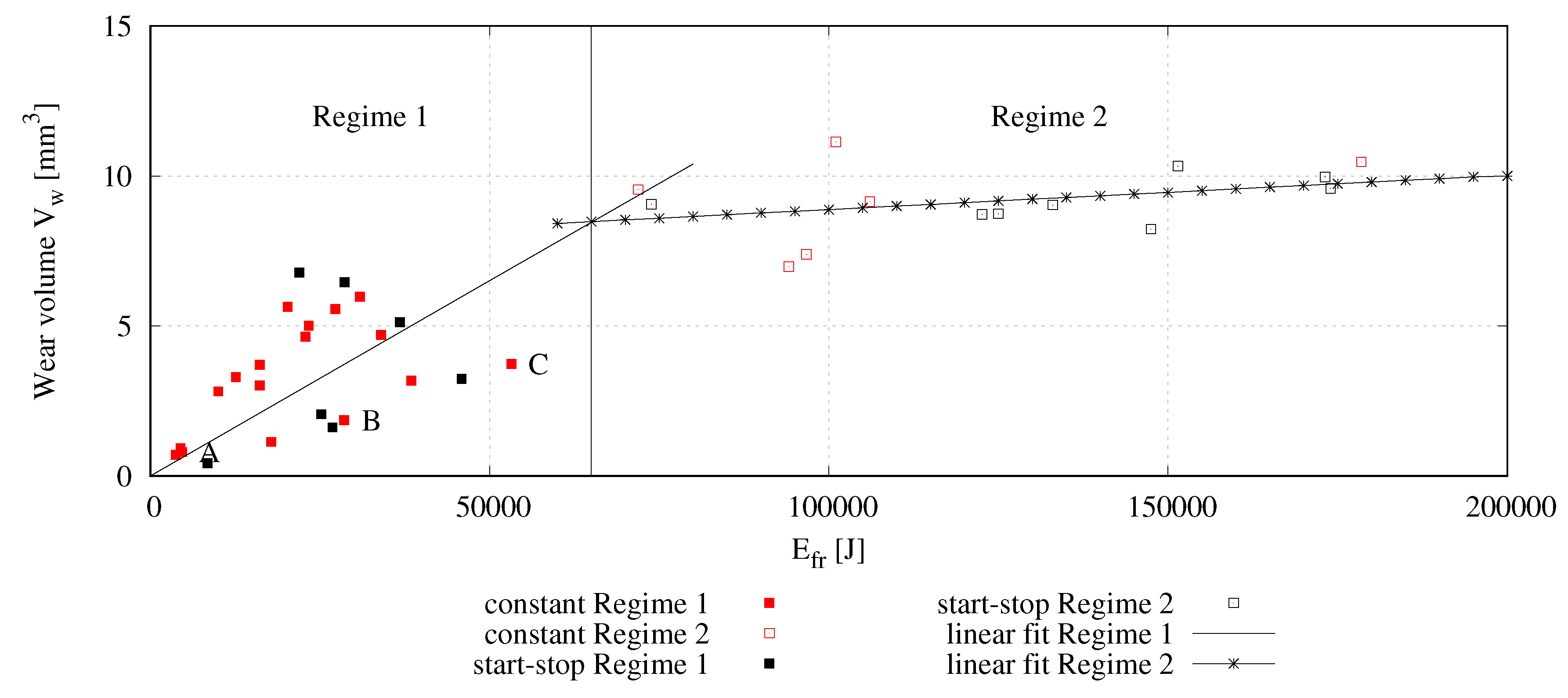
3.2. Wear Results
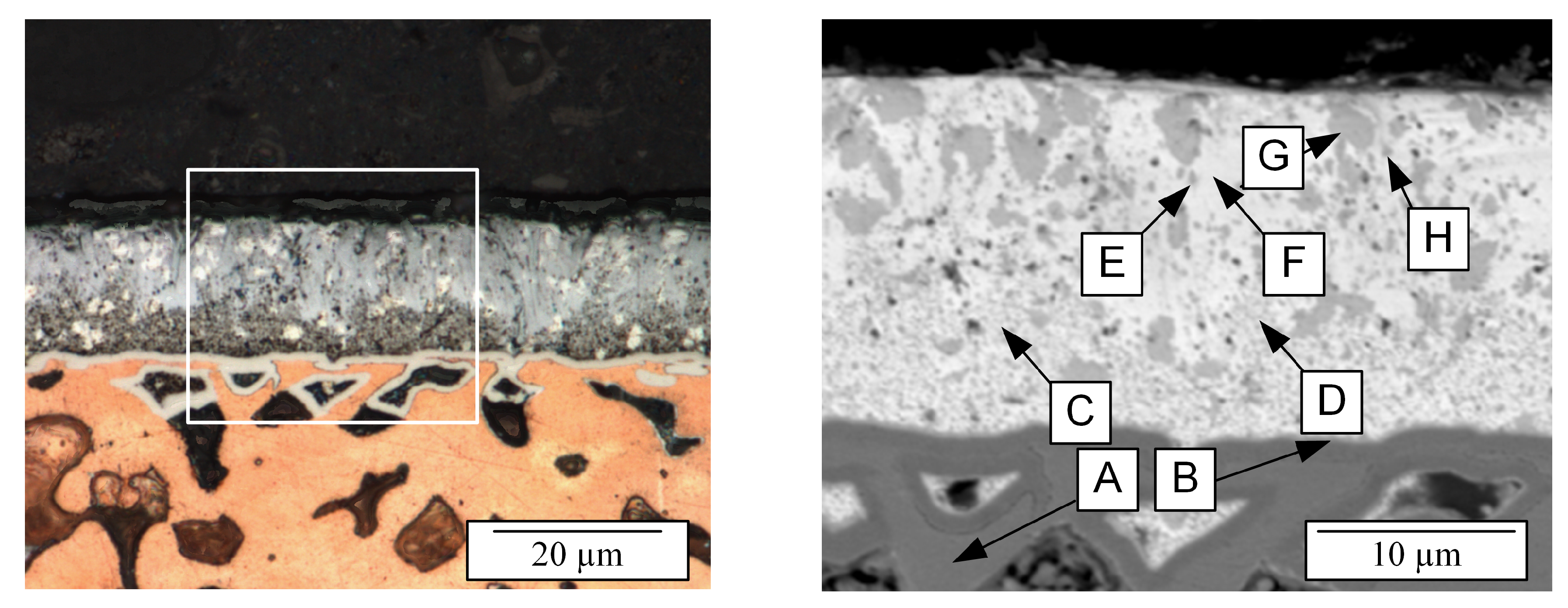
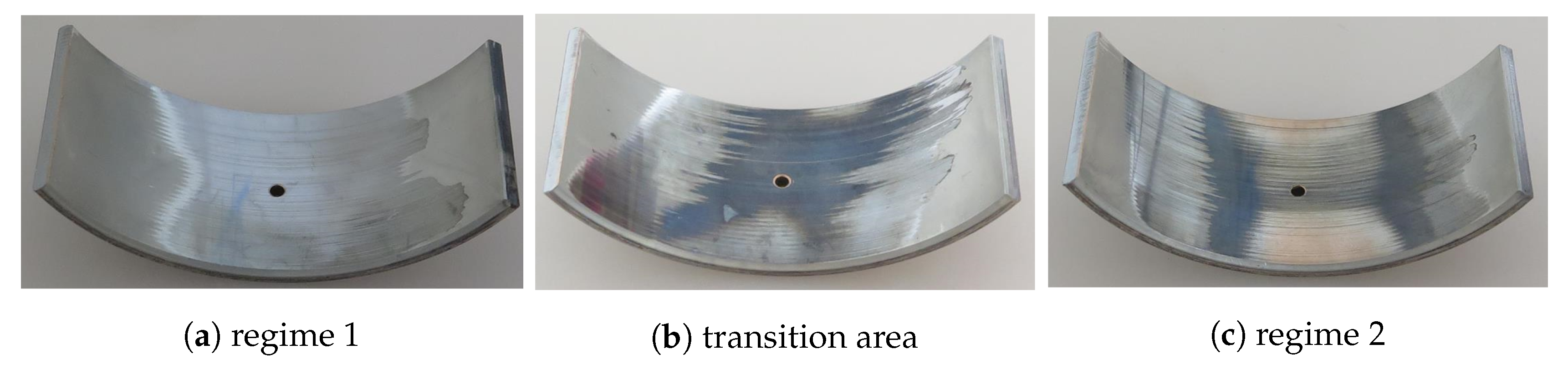
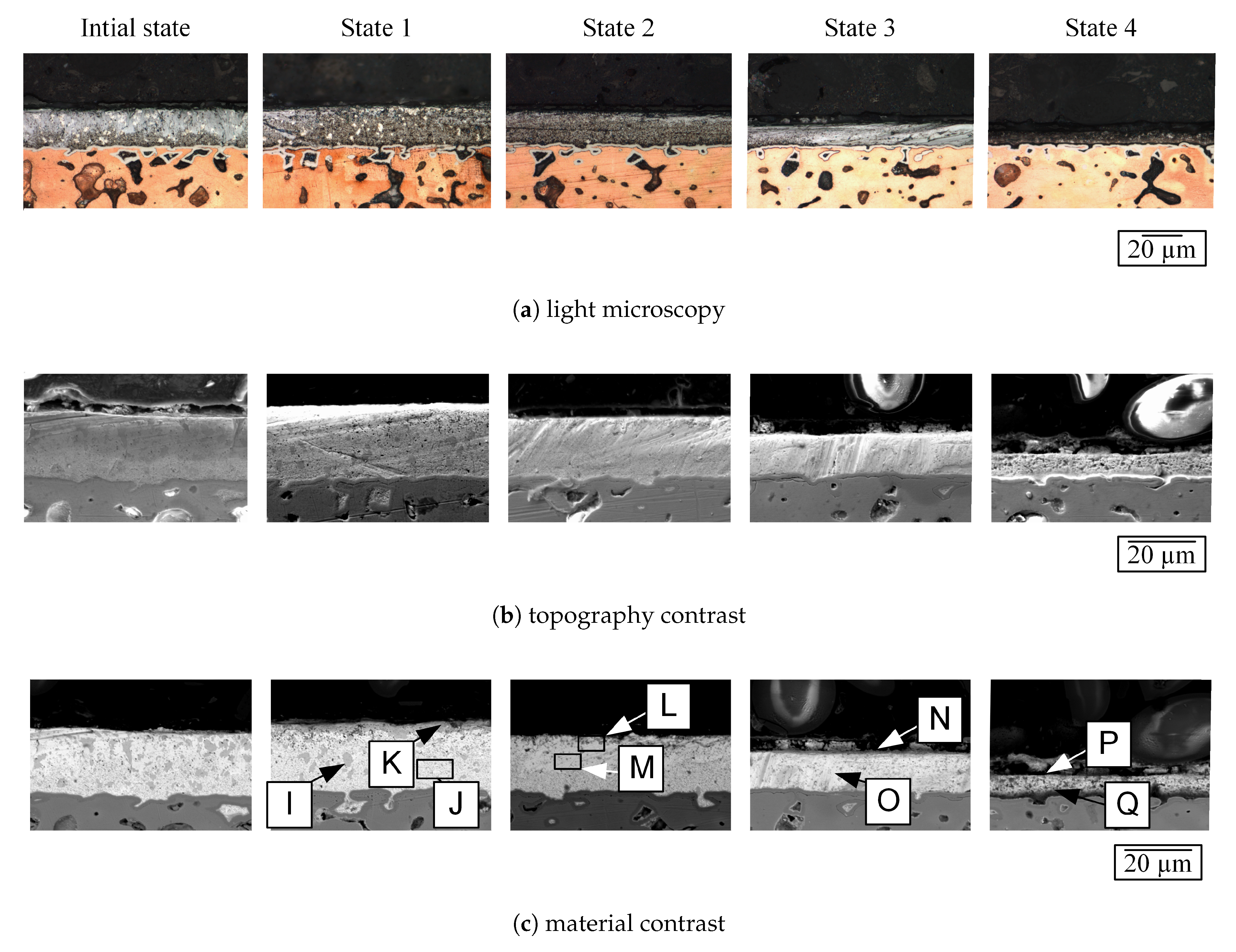
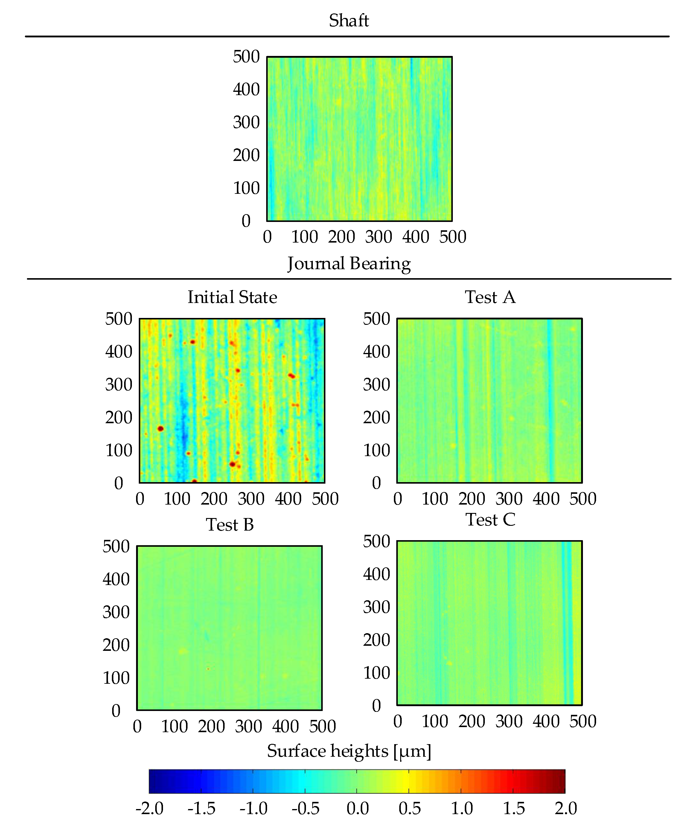
3.3. Surface Analysis
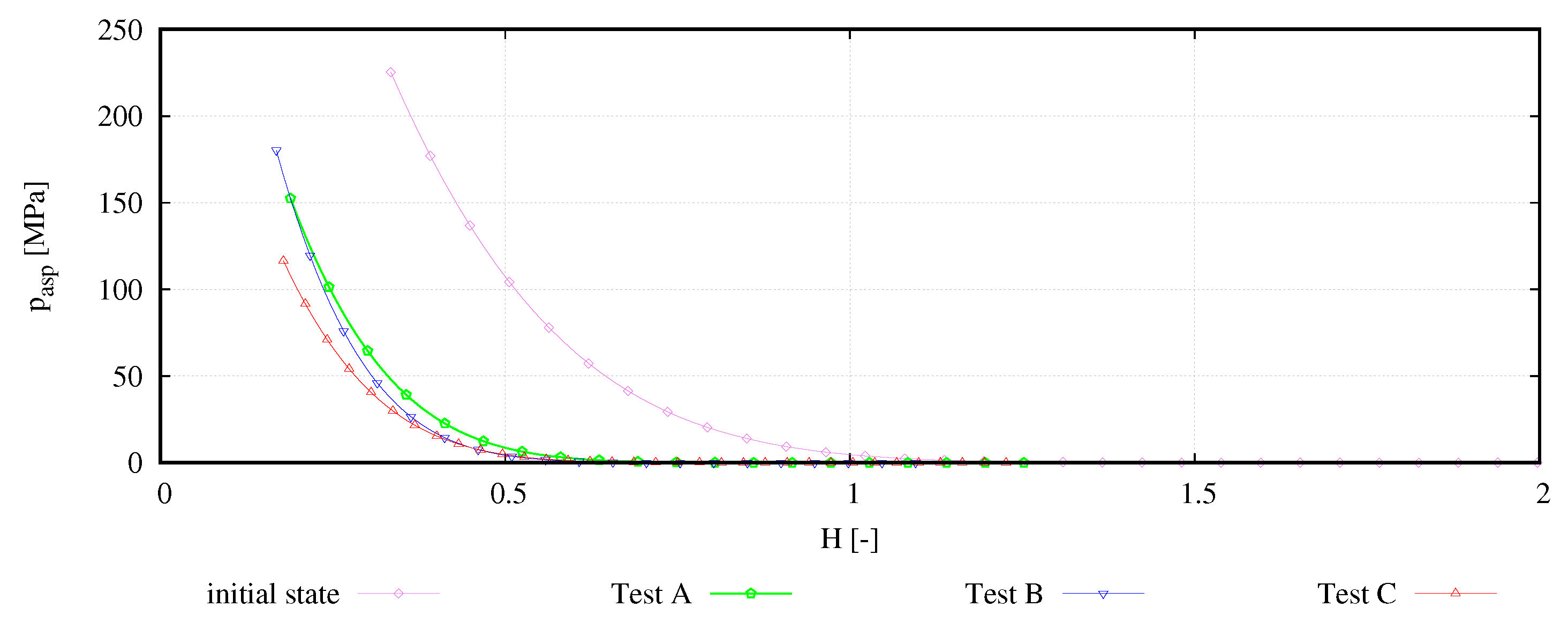
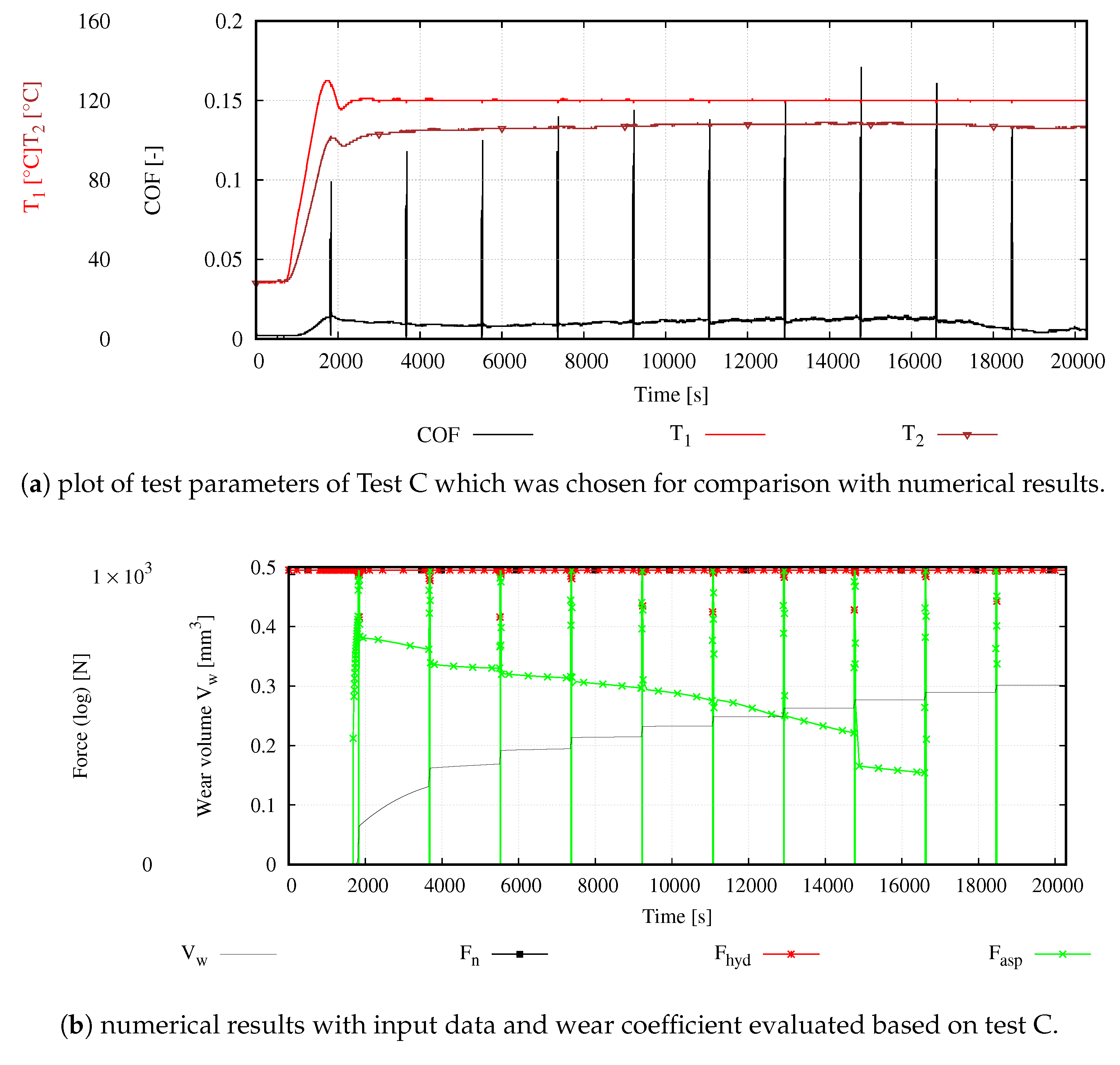
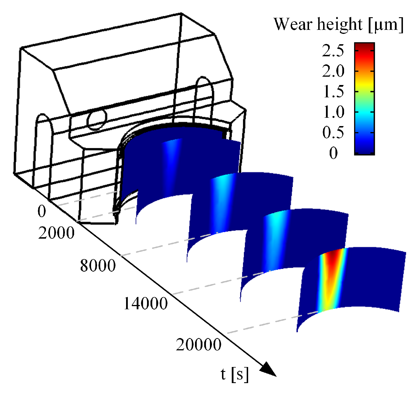
3.4. Numerical Evaluation
4. Conclusions
- The used test methodology in combination with the comprehensive surface analysis chain is capable of resolving the wear process of journal bearing specimens. With the help of this methodology, the process of wear and its effect on the tribological behaviour could be resolved in deep detail. By the use of the CP, the identification of different states of lubrication was enabled, which subsequently allowed a weighting of asperity contact intensity. In the following, this approach allowed for a coherent wear evaluation. For both test strategies which included two different types of loading conditions, the CP supported evaluation method provided a common scatter and correlated the same share of energy input for a resulting wear volume for both strategies, which points out the universal applicability of this method.
- The developed numerical framework represents the first approach concerning wear simulation in tribological contacts with COMSOL, which allows the simulation of operation in fluid and mixed lubrication and a simultaneous wear evaluation. The calculation can be conducted effectively and yields phenomenological comparable results to experimental data. However, a significant deviation in absolute numbers is evident. This can be mainly attributed to the used contact model and the evaluated wear intensity. As presented, a conservative contact model representing a run in state of surface was chosen. This leads to a general underestimation of asperity contact and, consequently, wear. The use of a contact model representing the initial surface state would increase the amount of wear but would not bring deeper insights. Hence, for a better estimation of wear, an additional feature which allows the consideration of a varying contact intensity dependent on the states of surface and wear is sought for the upcoming investigations, which will certainly increase the capability of wear prediction in absolute numbers.
- Special attention must also be given to the correlation function of the CP weighting. In the actual work, a linear correlation was chosen. The use of a different weighting function, which needs to be developed in agreement with test results, could certainly increase the significance of the numerical results.
Author Contributions
Funding
Acknowledgments
Conflicts of Interest
Abbreviations
| BSTA | Bearing segment test adapter |
| HSDA | High speed data acquisition mode |
| EDX | Energy dispersive X-ray spectroscopy |
| FEM | Finite element method |
| MUMPS | Multiftrontal massevily parallel sparse direct solver |
| SEM | Scanning electron microscope |
| EHL | Elastohydrodynamic lubrication |
| DOF | Degrees of freedom |
| CAD | Computer-aided design |
Nomenclature
| mean summit radius, µm | |
| mechanical strain, - | |
| lubricant viscosity, mPas | |
| summit density, m−2 | |
| orientation parameter, - | |
| Poisson’s ratio of surface material 1 and 2, - | |
| summit interface, µm | |
| standardized summit interface, - | |
| shear flow factor, - | |
| pressure flow factor, - | |
| lubricant density, kg/m3 | |
| standard deviation of surface heights (surface roughnes), µm | |
| standard deviation of summits heights, µm | |
| mechanical stress, MPa | |
| normalized summit height, - | |
| summit height measured from the mean summit plane, µm | |
| C | wear intensity, J/m3 |
| COF | coeffcient of friction, - |
| COF0 | maximum boundary coefficient of friction, - |
| CP | contact potential, mV |
| DOF | degree of freedom, - |
| E’ | combined Young’s modulus, GPa |
| E1,2 | Young’s modulus of surface material 1 and 2, GPa |
| Efr | frictional energy, J |
| F | loads within structual mechanics, N |
| Fasp | force resutling from asperity contact pressure, N |
| Fhyd | hydrodynamic force, N |
| Fn | normal force, N |
| H | normalized surface separation, - |
| h | fluid film gap height, m |
| h0 | initial lubrication gap height, m |
| h2 | wear height, m |
| K | empirical wear constant (Archard’s wear law), - |
| k | spring constant, N/m |
| pasp | asperity contact pressure, MPa |
| phyd | hydrodynamic pressure, MPa |
| pm | flow pressure of softer material in contact, MPa |
| pn | normal load, MPa |
| ps | scaling parameter, - |
| s | sliding distance, m |
| T1 | system temperature, C |
| T2 | contact close temperature, C |
| U1,2 | velocity of surface 1 and 2, m/s |
| ub,s | deformation of bearing and shaft, m |
| v | sliding speed, m/s |
| Vw | wear volume, m3 |
References
- Rozeanu, L.; Kennedy, F.E. Wear of hydrodynamic journal bearings. In Tribology Series; Dalmaz, G., Lubrecht, A.A., Dowson, D., Priest, M., Eds.; Elsevier: New York, NY, USA, 2001; Volume 39, pp. 161–166. [Google Scholar]
- Grün, F.; Gódor, I.; Gärtner, W.; Eichlseder, W. Tribological performance of thin overlays for journal bearings. Tribol. Int. 2011, 44, 1271–1280. [Google Scholar] [CrossRef]
- Grün, F.; Gódor, I.; Eichlseder, W. Test methods to characterise differently designed tribomaterials. Tribotest 2008, 14, 159–176. [Google Scholar] [CrossRef]
- Grün, F.; Summer, F.; Pondicherry, K.S.; Gódor, I.; Offenbecher, M.; Lainé, E. Tribological functionality of aluminium sliding materials with hard phases under lubricated conditions. Wear 2013, 298–299, 127–134. [Google Scholar] [CrossRef]
- Summer, F.; Grün, F.; Schiffer, J.; Gódor, I.; Papadimitriou, I. Tribological study of crankshaft bearing systems: Comparison of forged steel and cast iron counterparts under start–stop operation. Wear 2015, 338, 232–241. [Google Scholar] [CrossRef]
- Summer, F.; Grün, F.; Offenbecher, M.; Taylor, S.; Lainé, E. Tribology of journal bearings: Start stop operation as life-time factor. Tribol. Schmier. 2017, 64, 46–56. [Google Scholar]
- Farfán-Cabrera, L.I.; Gallardo-Hernández, E.A. Wear evaluation of journal bearings using an adapted micro-scale abrasion tester. Wear 2017, 376–377, 1841–1848. [Google Scholar] [CrossRef]
- Gebretsadik, D.W.; Hardell, J.; Prakash, B. Friction and wear characteristics of different Pb-free bearing materials in mixed and boundary lubrication regimes. Wear 2015, 340–341, 63–72. [Google Scholar] [CrossRef]
- Gebretsadik, D.W.; Hardell, J.; Prakash, B. Tribological performance of tin-based overlay plated engine bearing materials. Tribol. Int. 2015, 92, 281–289. [Google Scholar] [CrossRef]
- Taylor, C. Automobile engine tribology—Design considerations for efficiency and durability. Wear 1998, 221, 1–8. [Google Scholar] [CrossRef]
- Priest, M.; Taylor, C. Automobile engine tribology—Approaching the surface. Wear 2000, 241, 193–203. [Google Scholar] [CrossRef]
- Albers, A.; Reichert, S. On the influence of surface roughness on the wear behavior in the running-in phase in mixed-lubricated contacts with the finite element method. Wear 2017, 376–377, 1185–1193. [Google Scholar] [CrossRef]
- Põdra, P.; Andersson, S. Simulating sliding wear with finite element method. Tribol. Int. 1999, 32, 71–81. [Google Scholar] [CrossRef]
- Arjmandi, M.; Ramezani, M.; Giordano, M.; Schmid, S. Finite element modelling of sliding wear in three-dimensional woven textiles. Tribol. Int. 2017, 115, 452–460. [Google Scholar] [CrossRef]
- Reichert, S.; Lorentz, B.; Heldmaier, S.; Albers, A. Wear simulation in non-lubricated and mixed lubricated contacts taking into account the microscale roughness. Tribol. Int. 2016, 100, 272–279. [Google Scholar] [CrossRef]
- Khader, I.; Renz, A.; Kailer, A. A wear model for silicon nitride in dry sliding contact against a nickel-base alloy. Wear 2017, 376–377, 352–362. [Google Scholar] [CrossRef]
- Chun, S.M.; Khonsari, M.M. Wear simulation for the journal bearings operating under aligned shaft and steady load during start-up and coast-down conditions. Tribol. Int. 2016, 97, 440–466. [Google Scholar] [CrossRef]
- Archard, J.; Hirst, W. The wear of metals under unlubricated conditions. Proc. R. Soc. Lond. A 1956, 236, 397–410. [Google Scholar] [CrossRef]
- Aghdam, A.; Khonsari, M. Prediction of wear in grease-lubricated oscillatory journal bearings via energy-based approach. Wear 2014, 318, 188–201. [Google Scholar] [CrossRef]
- Sander, D.E.; Allmaier, H.; Priebsch, H.; Reich, F.; Witt, M.; Skiadas, A.; Knaus, O. Edge loading and running-in wear in dynamically loaded journal bearings. Tribol. Int. 2015, 92, 395–403. [Google Scholar] [CrossRef]
- Beheshti, A.; Khonsari, M.M. An engineering approach for the prediction of wear in mixed lubricated contacts. Wear 2013, 308, 121–131. [Google Scholar] [CrossRef]
- Mokhtar, M.O.A.; Howarth, R.B.; Davies, P.B. The Behavior of Plain Hydrodynamic Journal Bearings during Starting and Stopping. ASLE Trans. 1977, 20, 183–190. [Google Scholar] [CrossRef]
- Haneef, M.; Randall, R.; Smith, W.; Peng, Z. Vibration and wear prediction analysis of IC engine bearings by numerical simulation. Wear 2017, 384–385, 15–27. [Google Scholar] [CrossRef]
- Bergmann, P.; Grün, F.; Summer, F.; Gódor, I.; Stadler, G. Expansion of the Metrological Visualization Capability by the Implementation of Acoustic Emission Analysis. Adv. Tribol. 2017, 2017, 17. [Google Scholar] [CrossRef]
- Summer, F.; Bergmann, P.; Grün, F. Damage Equivalent Test Methodologies as Design Elements for Journal Bearing Systems. Lubricants 2017, 5, 47. [Google Scholar] [CrossRef]
- Reynolds, O. On the Theory of Lubrication and Its Application to Mr. Beauchamp Tower’s Experiments, Including an Experimental Determination of the Viscosity of Olive Oil. Philos. Trans. R. Soc. Lond. 1886, 177, 157–234. [Google Scholar] [CrossRef]
- Patir, N.; Cheng, H.S. An Average Flow Model for Determining Effects of Three-Dimensional Roughness on Partial Hydrodynamic Lubrication. J. Lubr. Technol. 1978, 100, 12–17. [Google Scholar] [CrossRef]
- Patir, N.; Cheng, H.S. Application of Average Flow Model to Lubrication Between Rough Sliding Surfaces. J. Lubr. Technol. 1979, 101, 220–229. [Google Scholar] [CrossRef]
- Bergmann, P.; Grün, F.; Gódor, I.; Stadler, G.; Maier-Kiener, V. On the modelling of mixed lubrication of conformal contacts. Tribol. Int. 2018, 125, 220–236. [Google Scholar] [CrossRef]
- Peklenik, J. New Developments in Surface Characterization and Measurements by Means of Random Process Analysis. Proc. Inst. Mech. Eng. 1967, 182, 108–126. [Google Scholar] [CrossRef]
- Cameron, A. Principles of Lubrication; Longman Publishing Group: Harlow, UK, 1986. [Google Scholar]
- Committee, A.I.H. ASM Handbook; ASM International: Almere, The Netherland, 1992; Volume 18. [Google Scholar]
- Dowson, D.; Higginson, G. Elasto-Hydrodynamic Lubrication; International Series On Materials Science and Technology; Pergamon Press: Oxford, UK, 1977. [Google Scholar]
- Allmaier, H.; Priestner, C.; Six, C.; Priebsch, H.H.; Forstner, C.; Novotny-Farkas, F. Predicting friction reliably and accurately in journal bearings—A systematic validation of simulation results with experimental measurements. Tribol. Int. 2011, 44, 1151–1160. [Google Scholar] [CrossRef]
- Gohar, R. Elastohydrodynamics; Computing in Engineering; Imperial College Press: London, UK, 2001. [Google Scholar]
- Spikes, H.A. Sixty years of EHL. Lubr. Sci. 2006, 18, 265–291. [Google Scholar] [CrossRef]
- Spikes, H.A. Basics of EHL for practical application. Lubr. Sci. 2015, 27, 45–67. [Google Scholar] [CrossRef]
- Sander, D.E.; Allmaier, H.; Priebsch, H.H.; Reich, F.M.; Witt, M.; Füllenbach, T.; Skiadas, A.; Brouwer, L.; Schwarze, H. Impact of high pressure and shear thinning on journal bearing friction. Tribol. Int. 2015, 81, 29–37. [Google Scholar] [CrossRef]
- Walters, K. The Importance and Measurement of Lubricant Rheology. In Thinning Films and Tribological Interfaces; Dowson, D., Priest, M., Taylor, C., Ehret, P., Childs, T., Dalmaz, G., Lubrecht, A., Berthier, Y., Flamand, L., Georges, J.M., Eds.; Tribology Series; Elsevier: New York, NY, USA, 2000; Volume 38, pp. 487–499. [Google Scholar] [CrossRef]
- Hamrock, B.; Schmid, S.; Jacobson, B. Fundamentals of Fluid Film Lubrication; Mechanical Engineering Fundamentals of Fluid Film Lubrication; CRC Press: Boca Raton, FL, USA, 2004. [Google Scholar]
- Greenwood, J.A.; Williamson, J.B.P. Contact of nominally flat surfaces. Proc. R. Soc. Lond. A 1966, 295, 300–319. [Google Scholar] [CrossRef]
- McCool, J.I. Comparison of models for the contact of rough surfaces. Wear 1986, 107, 37–60. [Google Scholar] [CrossRef]
- Kalin, M.; Pogačnik, A.; Etsion, I.; Raeymaekers, B. Comparing surface topography parameters of rough surfaces obtained with spectral moments and deterministic methods. Tribol. Int. 2016, 93, 137–141. [Google Scholar] [CrossRef]
- Preston, F.W. The Theory and Design of Plate Glass Polishing Machines. J. Soc. Glass Technol. 1927, 11, 214. [Google Scholar]


| Position | O | Pb | Cu | Sn | Ni | C |
|---|---|---|---|---|---|---|
| A | - | - | 100.0 | - | - | - |
| B | - | - | 8.3 | - | 91.7 | - |
| C | 16.8 | 50.5 | 16.2 | 16.6 | - | - |
| D | 14.5 | 49.4 | 18.3 | 17.8 | - | - |
| E | - | 6.9 | 50.4 | 42.7 | - | - |
| F | - | 93.7 | - | 6.3 | - | - |
| G | - | - | - | 100.0 | - | - |
| H | - | 13.1 | 49.4 | 37.4 | - | - |
| Position | O | Pb | Cu | Sn | Ni | C |
|---|---|---|---|---|---|---|
| I | 15.6 | - | 4.4 | 80.0 | - | - |
| J | 22.5 | 14.4 | 12.0 | 14.4 | - | - |
| K | 14.6 | - | 31.9 | 53.5 | - | - |
| L | - | 61.0 | 18.5 | 20.6 | - | - |
| M | - | 77.5 | 10.0 | 12.4 | - | - |
| N | 27.5 | 41.6 | 8.7 | 7.6 | - | - |
| O | - | 71.4 | 14.8 | 13.8 | - | - |
| P | 48.0 | 29.1 | 7.9 | 15.0 | - | - |
| Q | 40.6 | 34.4 | 13.1 | 11.9 | - | - |
© 2018 by the authors. Licensee MDPI, Basel, Switzerland. This article is an open access article distributed under the terms and conditions of the Creative Commons Attribution (CC BY) license (http://creativecommons.org/licenses/by/4.0/).
Share and Cite
Bergmann, P.; Grün, F.; Summer, F.; Gódor, I. Evaluation of Wear Phenomena of Journal Bearings by Close to Component Testing and Application of a Numerical Wear Assessment. Lubricants 2018, 6, 65. https://doi.org/10.3390/lubricants6030065
Bergmann P, Grün F, Summer F, Gódor I. Evaluation of Wear Phenomena of Journal Bearings by Close to Component Testing and Application of a Numerical Wear Assessment. Lubricants. 2018; 6(3):65. https://doi.org/10.3390/lubricants6030065
Chicago/Turabian StyleBergmann, Philipp, Florian Grün, Florian Summer, and István Gódor. 2018. "Evaluation of Wear Phenomena of Journal Bearings by Close to Component Testing and Application of a Numerical Wear Assessment" Lubricants 6, no. 3: 65. https://doi.org/10.3390/lubricants6030065