Abstract
This paper presents a multiscale finite element method applied to the simulation of a lubricating film flowing between rough surfaces. The objective of this approach is to study flows between large rough surfaces needing very fine meshes while maintaining a reasonable computation time. For this purpose, the domain is split into a number of subdomains (bottom-scale meshes) connected by a coarse mesh (top-scale). The pressure distribution at the top-scale is used as boundary conditions for the bottom-scale problems. This pressure is adjusted to ensure global mass flow balance between the contiguous subdomains. This multiscale method allows for a significant reduction of the number of operations as well as a satisfactory accuracy of the results if the top-scale mesh is properly fitted to the roughness lateral scale. Furthermore the present method is well-suited to parallel computation, leading to much more significant computation time reduction.
1. Introduction
The lubrication regime between surfaces in relative motion is controlled by the duty parameter , where is the lubricant viscosity, V the sliding speed, L the contact length and W the applied load [1]. When G is reduced, the friction decreases until asperity contact occurs and mixed lubrication begins. Reducing the viscosity of lubricants is a common solution used to decrease friction losses in engines [2] or other applications [3]. The decrease in leads to a reduction of G and of the thickness of the fluid film between the surfaces. As a consequence, the mixed lubrication tends to become the standard lubrication regime. It is thus of importance to have tools able to simulate this lubrication regime in a reasonable computation time and with sufficient accuracy.
The first step is the analysis of the flow between rough surfaces. The fluid flow is generally described using the Reynolds equation, which was initially solved assuming smooth surfaces [4]. The surface roughness must thus be taken into account in the model. One of the problems is that rough surfaces exhibit a multiscale nature, which makes their analysis and simulation difficult [5]. To get rid of this complexity, the first models developed in the 1960s assumed simplified geometric configurations. For example, Tzeng and Saibel [6] assumed one-directional striated surfaces. Using an averaging method, they were able to include correction factors in the Reynolds equation. Their approach was improved by Tonder [7]. To consider more complex surfaces with two-dimensional patterns, Patir and Cheng introduced the flow factor theory in the 1970s [8,9]. They used very small samples of rough surface on which they performed direct numerical simulations also called deterministic simulations. They obtained correction factors for the fluid flow that they incorporated in the averaged Reynolds equation. Their method had much success and was improved by several authors to derive the flow factors theoretically [10,11] or to include micro-cavitation [12]. Another method was developed meanwhile. Indeed, assuming that the roughness has a periodic pattern, it is possible to use the homogenization theory [13]. This method was extended to take account of cavitation [14], as well as the topography of real surfaces [15,16]. This approach was recently further improved with heterogenous homogenization [17,18]. However, all these averaging methods suffer a limitation. They are unable to simulate the load experimentally observed between nominally parallel flat surfaces [1].
With the development of computer capacities, it has been possible to perform deterministic simulations. Deterministic means that the conventional Reynolds equation is used while considering the real surface roughness. A very fine mesh is then used to capture the details of the topography of the rough surfaces. It was first used in point contacts [19] and later applied to line contacts [20]. More recently, the deterministic solution was used for conformal parallel surfaces [21]. It has been made possible to simulate the roughness-induced load generation between parallel surfaces. However, because of the required computation time, the studied surface was of limited extent, and periodical boundary conditions were used, which is not realistic.
There has been a great research effort to reduce the computation time for such problems and consider the multiscale nature of rough surfaces. One of the first efficient methods was based on the multi-grid techniques [22]. The principle is to use several mesh densities to remove low frequency residuals in order to accelerate the convergence. This method has been used by many authors [19,20] because of its efficiency. This method is, however, limited to structured regular meshes. A multiscale approach based on a solution combining two mesh levels was proposed by Neymeck et al. [23]. The macro-mesh pressure solution serves as boundary conditions for the micro-mesh. This pressure is adjusted to ensure global mass conservation between micro-subdomains. The method was however limited to an unidimensional macro-mesh and cannot be extended to large rough surfaces. More recently, Brunetiére and Wang [24] proposed a mixed solution. The method consists of combining an averaging method for the high frequencies of the roughness and a deterministic solution for the low frequencies. This approach however relies on a filtering process, which can be difficult to perform.
The present paper proposes to extend the initial multiscale principle proposed by Nyemeck et al. [23] to a two-dimensional problem discretized with the finite element method. First, the method is presented. Then, some results showing its performance in terms of reducing the computation time are presented for the case of hydrodynamic lubrication between rigid rough surfaces. Finally, the accuracy of the method is discussed.
2. Theoretical Approach
2.1. Configuration of the Problem
The configuration of the studied problem is presented in Figure 1. A rigid smooth surface is moving along the -axis at a constant speed V. A stationary and rigid rough surface of size by is placed at the average distance from the bottom surface. A viscous fluid separates the two surfaces.
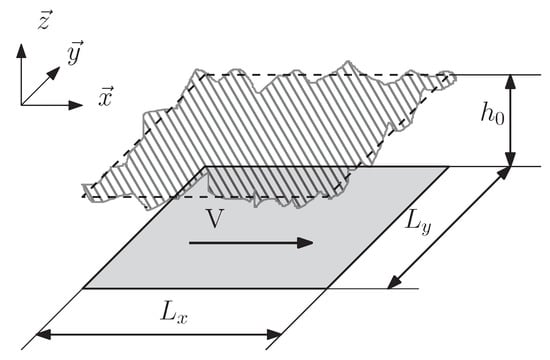
Figure 1.
Configuration of the problem.
The fluid flow between the surfaces is in steady state and governed by the following Reynolds equation:
where h is the local film thickness, is the viscosity of the fluid, is the density of the fluid, and p is the pressure, which is the unknown of the problem. The film thickness is defined as , where is the roughness of the surface. The usual lubrication assumptions ( and , continuous media, laminar flow, fluid inertia neglected, constant properties through the film thickness, no slip on the walls) hold to obtain this equation. Some additional hypotheses are used:
- The fluid is incompressible;
- There is no film rupture or cavitation;
- Thermal effects are neglected;
- The surfaces are rigid.
These assumptions, even if not realistic, are used in this initial work because the aim of the paper is to focus on the multiscale method. Considering a multiphysics problem would make the discussion on the model performance more difficult.
2.2. Finite Element Formulation
The Reynolds equation is multiplied by a weighting function and is integrated over the whole domain. It constitutes a residual:
An integration by parts is then carried out to reduce the order of the derivatives with respect to the pressure. A weak formulation is then obtained:
The second term is the mass flow rate along the boundary weighted by the function .
The domain is split into isoparametric elements with n nodes. The Bubnov–Galerkin method is used, meaning that the weighting functions are chosen equal to the shape function of the elements [25]. Using the n shape functions of the n nodes, n equations are obtained. Since the pressure is known along the boundary of the domain, it is not necessary to use equations for the nodes located on the boundary of the domain. Thus, the shape functions vanish along the boundary as well as the boundary integral in Equation (3).
Even if the problem is linear, it is useful to consider the more general nonlinear case for situations such as compressible fluids or cavitation. The Newton–Raphson method leads to the following set of equations:
where is the pressure at node j and a pressure variation.
This system of equations is solved using two different direct solvers. The multi-frontal UMFPack (http://faculty.cse.tamu.edu/davis/suitesparse.html) solver in its single-threaded version is used as well as the parallel solver MUMPS (http://mumps.enseeiht.fr/). The two packages are solvers for systems of linear equations with sparse matrices. A Gaussian elimination is performed by transforming the matrix in the product of a lower triangular matrix L by an upper triangular matrix U using multi-frontal methods. The solution is obtained in three steps. First, the system is analyzed and a symbolic factorization is performed. For a given shape of the matrix—non zero locations—the analysis is done once. During the second step, the matrix is numerically factorized, leading to L and U matrices. Finally the system is solved. These two solvers are called from a unique interface, MSOLV (https://tribo-pprime.github.io/MSOLV/index.html).
2.3. Multiscale Approach
As shown in Figure 2, the regular method consists of solving the problem equations on a fine mesh containing elements and covering the whole domain. In the multiscale approach, the domain is first discretized with a coarse mesh. It is the macro scale or top-scale. The number of elements of this mesh is denoted by . Each of the elements is then finely meshed. This is the micro scale or bottom-scale. In the present paper, all the top elements have the same size, and all the subdomains have the same number of elements . The following relationship between the number of elements is finally obtained:
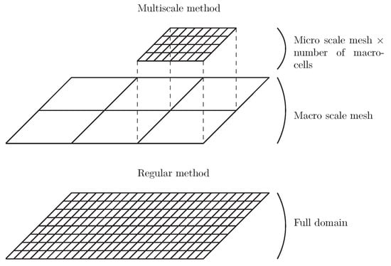
Figure 2.
multiscale mesh.
The calculation principle and the solution procedure of the multiscale method are described in Figure 3. An initial guess of the pressure distribution is first assumed at the top-scale (it can be a uniform pressure distribution). This pressure distribution is then used as boundary conditions for the micro scale problems. The pressure solutions at the bottom-scale are obtained using the approach presented in Section 2.2. Note that there are independent subproblems to be solved simultaneously. Knowing the pressure distributions at the bottom-scale, it is then possible to calculate the mass flow rate along the boundary of the subdomains:
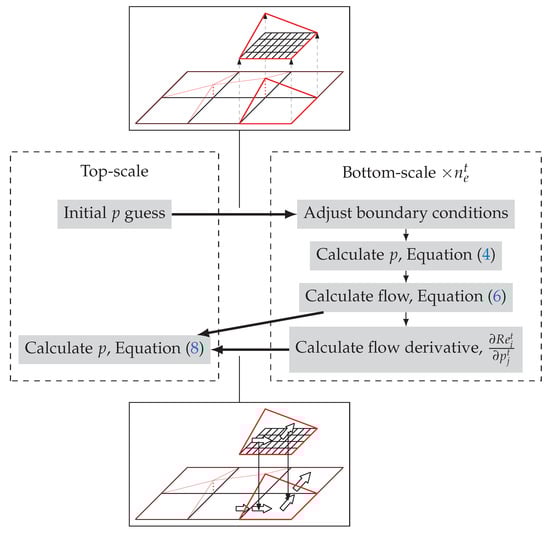
Figure 3.
Multiscale solution procedure.
In this equation, is the top-scale shape function. There is thus one flow rate value per top-scale node. These flow rates are exported to the top-scale where they are summed to obtain the residual flow rate for each top-scale node:
By making small variations in the pressure at the boundaries of the bottom-scale problems, derivatives of the flow rate with respect to the pressure can be calculated. Since only the right-hand sides of the system of equations are modified, the solution is obtained very quickly. Finally, the pressure at the top-scale is adjusted to ensure mass flow balance between contiguous elements. This means that the flow rate residuals must vanish:
Since the problem is linear, the solution at the top-scale is obtained after one iteration at the bottom-scale (regardless of the initial pressure estimate). If the pressure at the bottom-scale is required, for example to calculate the load, a second simulation is performed at the bottom-scale with the new pressure distribution from the top-scale. Note that when cavitation is included, several iterations are necessary because of the nonlinear behavior of the problem.
The scale transition is ensured by assuming a linear pressure distribution along the bottom-scale domains and a global mass conservation between the elements at the top-scale. Local mass conservation is not ensured between contiguous subdomains. These are the main simplifications involved in the present approach. They allow decreasing the computation time but they induce errors in the pressure solution compared to the global deterministic solution.
Finally, it should be noted that the algorithm was coded with modern Fortran language.
3. Results
The configuration used for the problem is presented in Figure 1 and the parameters are given in Table 1. The rough surface used in the simulation is presented in Figure 4. It is a numerically- simulated 2048 × 2048 bi-Gaussian surface, which is typical of surfaces used in tribological applications [26]. This isotropic surface has a smooth plateau with deep valleys, as indicated by the values of and in Table 1. Simulated surfaces are used in this work because it is possible to accurately control their statistical properties. However, a measured surface could also be used. The film thickness is chosen to avoid any asperity contact, something which is not addressed in the present paper. The surface is divided in k = 2–512 subdomains per side for the multiscale simulation. Because of the square shape of the problem, . The fluid is assumed to be incompressible and cavitation is neglected in this initial approach. The pressure is equal to zero along the boundary. The resulting pressure is proportional to a reference hydrodynamic pressure:
where is the width of the domain. Note that a square shape was used to simplify the analysis of the results but, more generally speaking, the finite element method used in the model allows for high flexibility in the shape of the domain.

Table 1.
Geometrical configuration of the problem.
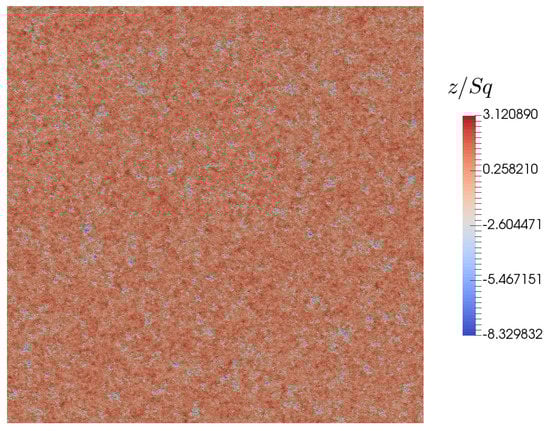
Figure 4.
Rough surface used in the simulation.
The pressure distributions obtained with the deterministic solution and with the multiscale solution with are presented in Figure 5. The top-scale pressure gives the main trends of the pressure field obtained with the full solution, while the details are obtained at the bottom level. The bottom-scale solution appears to be very close to the deterministic solution even if there are some differences along the edges of the subdomain where linear pressure boundary conditions are imposed.
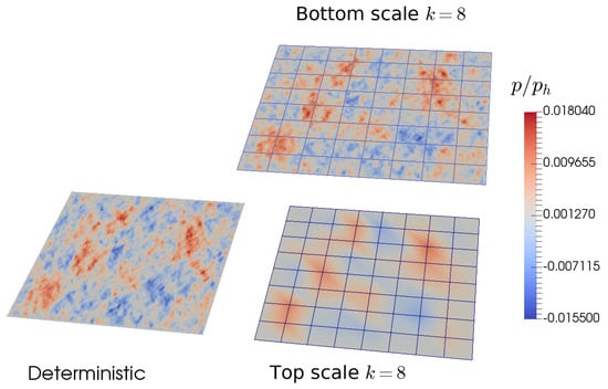
Figure 5.
Comparison of the deterministic and multiscale pressure distributions.
The objective of the multiscale approach is to reduce the computation time. To asses the efficiency of the method, two types of calculation are performed. First, the mono-processor solver UMFPack was used to solve both the bottom- and top-scale problems. Second, the multiprocessor solver MUMPS was used for the top-scale whereas the mono-processor solver was used in concurrent threads for the bottom-scale problems. Indeed, since there were independent bottom-scale problems to solve, this can be done in parallel using the Open-MP library. For the deterministic full solution (), only MUMPS was able to solve the problem because its 64 bits integer implementation allows for large memory allocation. The computation time obtained in this case was used as a reference.
Figure 6 presents the evolution of the computation time regarding the number of subdomains per side, for both the cases of sequential and parallel computations. The curves exhibit the same behavior: the computation time decreased when the number of subdomains was increased, then it reached a plateau. Based on the parallel computation curve, it can be shown that the present method could divide the computation time by about a factor of 13 when compared to the deterministic solution. The use of parallel computation could reduce the computing time by an additional factor. In the present case, where eight threads were used, this factor was about four. The multiscale approach was thus very effective at reducing the calculation time.
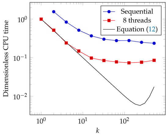
Figure 6.
Computation time as a function of the number of subdomains per side k.
Because of the linear pressure distribution assumed along the edges of the subdomains, some error on the pressure distribution was to be expected. The overall errors were assessed by using the calculated load, which was the integral of the pressure over the domain. Figure 7 presents the value of the load versus the number of subdomains per side, k. The load was normalized by the value obtained with the exact deterministic solution. At low values of k, there was a significant error, which could be higher than 50%. This error tended to decrease when k increased. A small error was obtained for the highest value of k.
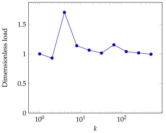
Figure 7.
Calculated load as a function of the number of subdomains per side k.
The results shown in Figure 7 are not surprising because when k increases the top-scale mesh is able to capture almost all the details of the exact solution. An illustration of this assertion is given in Figure 8. When k was small, the pressure distribution was almost uniform on the whole top-scale domain. When k was increased, the details of the pressure distribution appeared more clearly at the top-scale, leading to better boundary conditions for the bottom-scale problems, and hence a better accuracy.
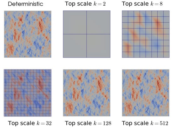
Figure 8.
Comparison of the deterministic and top-scale pressure distributions with different values of k.
4. Discussion
4.1. Computation Time
The computation time to solve a set of equations is directly linked to the number of operations to factorize the system. According to Duff [27], the number of operations or flops for a sparse system of N unknowns can be approximated by
Using an advanced method that includes an analysis step makes the number of flops decrease: [28]
In the case of a large domain, such as in the present problem, N is approximately equal to the number of elements of the domain , and the number of flops is . When the multiscale approach is used, there is one domain with elements and domains of elements. Thus the number of flops is
This equation is plotted in Figure 6 with and and after normalization by . This equation is able to describe the significant decrease of the computation time observed when k is increased from 1 to 8. Based on this theory, the number of flops and thus the computation time should be reduced by about 2 orders of magnitude when the number of subdomains is set at its optimal value, . In the present case, the reduction is by one order of magnitude and the optimal value is . The difference between the theory and the real computation time and more particularly the appearance of the plateau can be explained as follows. When k increases, the size of the bottom-scale matrices decreases. Thus, their sparsity (i.e., the ratio of the number of terms in the matrix to the number of non-zero terms) becomes lower and the efficiency of the solver algorithm is lowered with a number of flops tending to , which is higher than the expected .
4.2. Accuracy of the Method
It has been shown that the accuracy of the method depends on the number of subdomains used in the multiscale approach. The accuracy will be improved if the top-scale mesh is able to capture the main features of the pressure distribution. These features are expected to vary with the lateral size of the surface asperities. To analyze this assumption, several surfaces with different correlation lengths (expressed by according to the ISO standard 25178) were generated and used in the simulations. The effect of on the lateral size of the surface asperities is clearly visible in Figure 9. In addition, a second surface having the same statistical properties () as the reference surface was also generated.
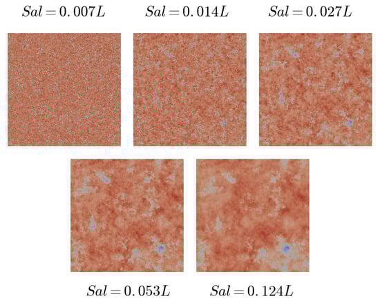
Figure 9.
The different surfaces used for the accuracy analysis.
For each of the six surfaces (the reference surface and five others), the deterministic solution was computed for a reference. Then, multiscale simulations were performed with different k values between two and 512, and the relative error of the computed load was calculated. In Figure 10, this relative error is presented as a function of the ratio of the correlation length to the size of the subdomain. Even if for a given surface, the evolution is not monotonic, a general trend can be observed. The error tends to decrease when the size ratio increases. Indeed, the top- scale mesh is able to capture more accurately the details of the pressure distribution. Moreover, a decrease in the slope is observed when the size ratio is approximately equal to one. This means that when the subdomains have a size less than the correlation length of the surface, the error decreases more rapidly. To reach an error of about 0.01, the size of the subdomain must be less than one-half the correlation length of the surface roughness. Thus, this gives a quantitative indicator for the discretization of the problem. This value can be compared to the optimal number of subdomains given by Equation (12) to find the best compromise in terms of accuracy and computation time. In the reference case, , this rule suggests the use of . This corresponds to the plateau zone where the computation time is minimal (see Figure 6).
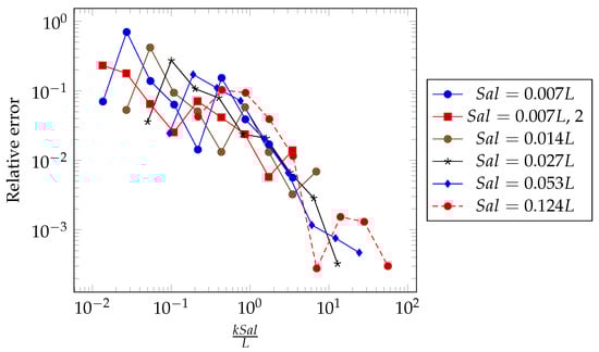
Figure 10.
Relative error in the load as a function of the ratio of the surface correlation length to the sub-domain size.
5. Conclusions
A multiscale finite element solution of the Reynolds equation was presented with the aim of studying the fluid flow between rough surfaces demanding very fine meshes. The domain is split into a number of subdomains (bottom-scale mesh) connected by a coarse mesh (top-scale). The pressure distribution at the top-scale is used as boundary conditions for the bottom-scale problems. This pressure is adjusted to ensure the global mass flow balance between contiguous subdomains.
This multiscale method allows for a significant reduction in the number of operations. In the example presented, the computation time was reduced by a factor of 13 from that needed by the full deterministic solution. Because each bottom-scale problem can be solved independently, parallel computation can be easily performed to further reduce the calculation time. The simplifications used to connect the subdomains induce some error, which can be maintained below 1% if the size of the subdomains is less than one-half the correlation length of the surface roughness.
There are several ways to further develop this method. For example, it can be applied to unstructured meshes with triangular elements and triangular subdomains. The size of the subdomains can be automatically adjusted depending on the surface parameters. The next step is now to include the occurrence of cavitation, which is mandatory when the lubrication regime is mixed. Another point to consider is transient problems appearing when the two surfaces are rough, as well as the squeeze effect.
Author Contributions
N.B. developed the multiscale method. A.F. developed the interface for the solvers used in the multiscale model. N.B. and A.F. performed the simulations, analyzed the data, and wrote the paper.
Funding
This research received no external funding.
Conflicts of Interest
The authors declare no conflict of interest.
References
- Lebeck, A. Parallel Sliding Load Support in the Mixed Friction Regime. Part 1—The Experimental Data. J. Tribol. 1987, 109, 189–195. [Google Scholar] [CrossRef]
- Holmberg, K.; Andersson, P.; Erdemir, A. Global energy consumption due to friction in passenger cars. Tribol. Int. 2012, 47, 221–234. [Google Scholar] [CrossRef]
- Holmberg, K.; Erdemir, A. Influence of tribology on global energy consumption, costs and emissions. Friction 2017, 5, 263–284. [Google Scholar] [CrossRef]
- Reynolds, O. On the Theory of Lubrication and Its Application to Mr. Beauchamp Tower’s Experiments, Including an Experimental Determination of the Viscosity of Olive Oil. Philos. Trans. R. Soc. Lond. 1886, 177, 157–234. [Google Scholar] [CrossRef]
- Bhushan, B. Chapter 2—Surface Roughness Analysis and Measurement Techniques. In Modern Tribology Handbook; CRC Press: Boca Raton, FL, USA, 2001; pp. 1–71. [Google Scholar]
- Tzeng, S.; Saibel, E. Surface Roughness Effect on Slider Bearing Lubrication. ASLE Trans. 1967, 10, 334–348. [Google Scholar] [CrossRef]
- Tonder, K. The Lubrication of Unidirectional Striated Roughness: Consequences for some General Roughness Theories. J. Tribol. 1986, 108, 167–170. [Google Scholar] [CrossRef]
- Patir, N.; Cheng, H. Application of Average Flow Model to Lubrication Between Rough Sliding Surfaces. J. Lubr. Technol. 1979, 101, 220–230. [Google Scholar] [CrossRef]
- Patir, N.; Cheng, H. An Average Flow Model for Determining Effects of Three-Dimensional Roughness on Partial Hydrodynamic Lubrication. J. Lubr. Technol. 1978, 100, 12–17. [Google Scholar] [CrossRef]
- Elrod, H. A General Theory for Laminar Lubrication With Reynolds Roughness. J. Lubr. Technol. 1979, 101, 8–14. [Google Scholar] [CrossRef]
- Tripp, J. Surface Roughness Effects in Hydrodynamic Lubrication: The Flow Factor Method. J. Lubr. Technol. 1983, 105, 458–465. [Google Scholar] [CrossRef]
- Harp, S.; Salant, R. An Average Flow Model of Rough Surface Lubrication With Inter-Asperity Cavitation. J. Tribol. 2001, 123, 134–143. [Google Scholar] [CrossRef]
- Bayada, G.; Faure, J. A Double Scale Analysis Approach of the Reynolds Roughness—Comments and Application to the Journal Bearing. J. Tribol. 1989, 111, 323–330. [Google Scholar] [CrossRef]
- Bayada, G.; Martin, S.; Vasquez, C. An Average Flow Model of the Reynolds Roughness Including a Mass-Flow Preserving Cavitation Model. J. Tribol. 2005, 127, 797–802. [Google Scholar] [CrossRef]
- Sahlin, F.; Larrson, R.; Almqvist, A.; Lugt, P.; Marklund, P. A Mixed Lubrication Model Incorporating Measured Surface Topography. Part 1: Theory of Flow Factors. IMechE Part J J. Eng. Tribol. 2010, 224, 335–351. [Google Scholar] [CrossRef]
- Sahlin, F.; Larrson, R.; Almqvist, A.; Lugt, P.; Marklund, P. A Mixed Lubrication Model Incorporating Measured Surface Topography. Part 2: Roughness Treatment, Model Validation, and Simulation. IMechE Part J J. Eng. Tribol. 2010, 224, 353–365. [Google Scholar] [CrossRef]
- De Boer, G.; Hewson, R.; Thompson, H.; Gao, L.; Toropov, V. Two-scale EHL: Three-dimensional topography in tilted-pad bearings. Tribol. Int. 2014, 79, 111–125. [Google Scholar] [CrossRef]
- Pérez-Ràfols, F.; Larsson, R.; Lundström, S.; Wall, P.; Almqvist, A. A stochastic two-scale model for pressure-driven flow between rough surfaces. Proc. R. Soc. Lond. A Math. Phys. Eng. Sci. 2016, 472. [Google Scholar] [CrossRef] [PubMed]
- Lubrecht, A.; Ten Napel, W.; Bosma, R. The Influence of Longitudinal and Transverse Roughness on the Elastohydrodynamic Lubrication of Circular Contacts. J. Tribol. 1988, 110, 421–426. [Google Scholar] [CrossRef]
- Ai, X.; Cheng, H. A Transient EHL Analysis for Line Contacts with Measured Surface Roughness Using Multigrid Technique. J. Tribol. 1994, 116, 549–556. [Google Scholar] [CrossRef]
- Minet, C.; Brunetière, N.; Tournerie, B. A Deterministic Mixed Lubrication Model for Mechanical Seals. J. Tribol. 2011, 133, 042203. [Google Scholar] [CrossRef]
- Lubrecht, T.; Venner, C. Multi-Level Methods in Lubrication; Elsevier: Amsterdam, The Netherlands, 2000; p. 400. [Google Scholar]
- Nyemeck, A.; Brunetière, N.; Tournerie, B. A Multiscale Approach to the Mixed Lubrication Regime: Application to Mechanical Seals. Tribol. Lett. 2012, 47, 417–429. [Google Scholar] [CrossRef]
- Brunetiére, N.; Wang, Q. Large-Scale Simulation of Fluid Flows for Lubrication of Rough Surfaces. J. Tribol. 2014, 136, 011701. [Google Scholar] [CrossRef]
- Zienkiewicz, O.; Taylor, R. The Finite Element Method, 5th ed.; Volume 1: The Basis; Butterworth Heinemann: Oxford, UK, 2000. [Google Scholar]
- Hu, S.; Huang, W.; Brunetiere, N.; Song, Z.; Liu, X.; Wang, Y. Stratified effect of continuous bi-Gaussian rough surface on lubrication and asperity contact. Tribol. Int. 2016, 104, 328–341. [Google Scholar] [CrossRef]
- Duff, I.S. A review of frontal methods for solving linear systems. Comput. Phys. Commun. 1996, 97, 45–52. [Google Scholar] [CrossRef]
- Xia, J.; Chandrasekaran, S.; Gu, M.; Li, X. Superfast Multifrontal Method for Large Structured Linear Systems of Equations. SIAM J. Matrix Anal. Appl. 2010, 31, 1382–1411. [Google Scholar] [CrossRef]


© 2018 by the authors. Licensee MDPI, Basel, Switzerland. This article is an open access article distributed under the terms and conditions of the Creative Commons Attribution (CC BY) license (http://creativecommons.org/licenses/by/4.0/).