Adhesion and Friction for Three Tire Tread Compounds


1
Apollo Tyres Global R&D B.V., P.O. Box 3795, 7500 DT|Colosseum 2, 7521 PT Enschede, The Netherlands
2
PGI-1, FZ Jülich, 52425 Jülich, Germany
3
MultiscaleConsulting, Wolfshovener Str 2, 52428 Jülich, Germany
*
Author to whom correspondence should be addressed.
Lubricants 2019, 7(3), 20; https://doi.org/10.3390/lubricants7030020
Submission received: 29 January 2019
/
Revised: 14 February 2019
/
Accepted: 16 February 2019
/
Published: 26 February 2019
(This article belongs to the Special Issue Adhesion, Friction and Lubrication of Viscoelastic Materials)
Abstract
:We study the adhesion and friction for three tire tread rubber compounds. The adhesion study is for a smooth silica glass ball in contact with smooth sheets of the rubber in dry condition and in water. The friction studies are for rubber sliding on smooth glass, concrete, and asphalt road surfaces. We have performed the Leonardo da Vinci-type friction experiments and experiments using a linear friction tester. On the asphalt road, we also performed vehicle breaking distance measurements. The linear and non-linear viscoelastic properties of the rubber compounds were measured in shear and tension modes using two different Dynamic Mechanical Analysis (DMA) instruments. The surface topography of all surfaces was determined using stylus measurements and scanned-in silicon rubber replicas. The experimental data were analyzed using the Persson contact mechanics and rubber friction theory.
1. Introduction
The friction and adhesion between rubber materials and a counter surface has many practical applications, e.g., for tires, conveyor belts, rubber seals, and pressure-sensitive adhesives. In these applications, the surface roughness of the rubber and the counter have a crucial influence on the contact mechanics [1,2,3,4,5]. However, the contact mechanics of filled rubber compounds is a very complex topic because of non-linearity [6,7], the temperature and frequency dependencies of the rubber viscoelastic modulus, and because all solids have surface roughness, usually extending from the linear size of the object down to atomic distances [8].
In this paper, we study the adhesion and sliding friction for three tire tread compounds denoted as A, B and C. B is a summer tread compound filled with carbon black. A is a summer tread compound filled with silica and containing a traction resin. C is a winter tread compound, filled with silica and containing the same traction resin (in the same relative volume fraction) as for Compound A.
We have measured the adhesion between these rubber compounds and a smooth glass sphere in dry state and in water. The sliding friction experiments were performed with the Leonardo da Vinci and linear friction testers, using as substrates smooth glass and concrete surfaces, both for the dry condition and in water. For the C compound, we also measured friction using a low temperature linear slider setup, for temperatures from to +. Friction experiments were also performed on an asphalt road track using the linear friction tester and vehicle braking experiments.
2. Surface Roughness Power Spectrum
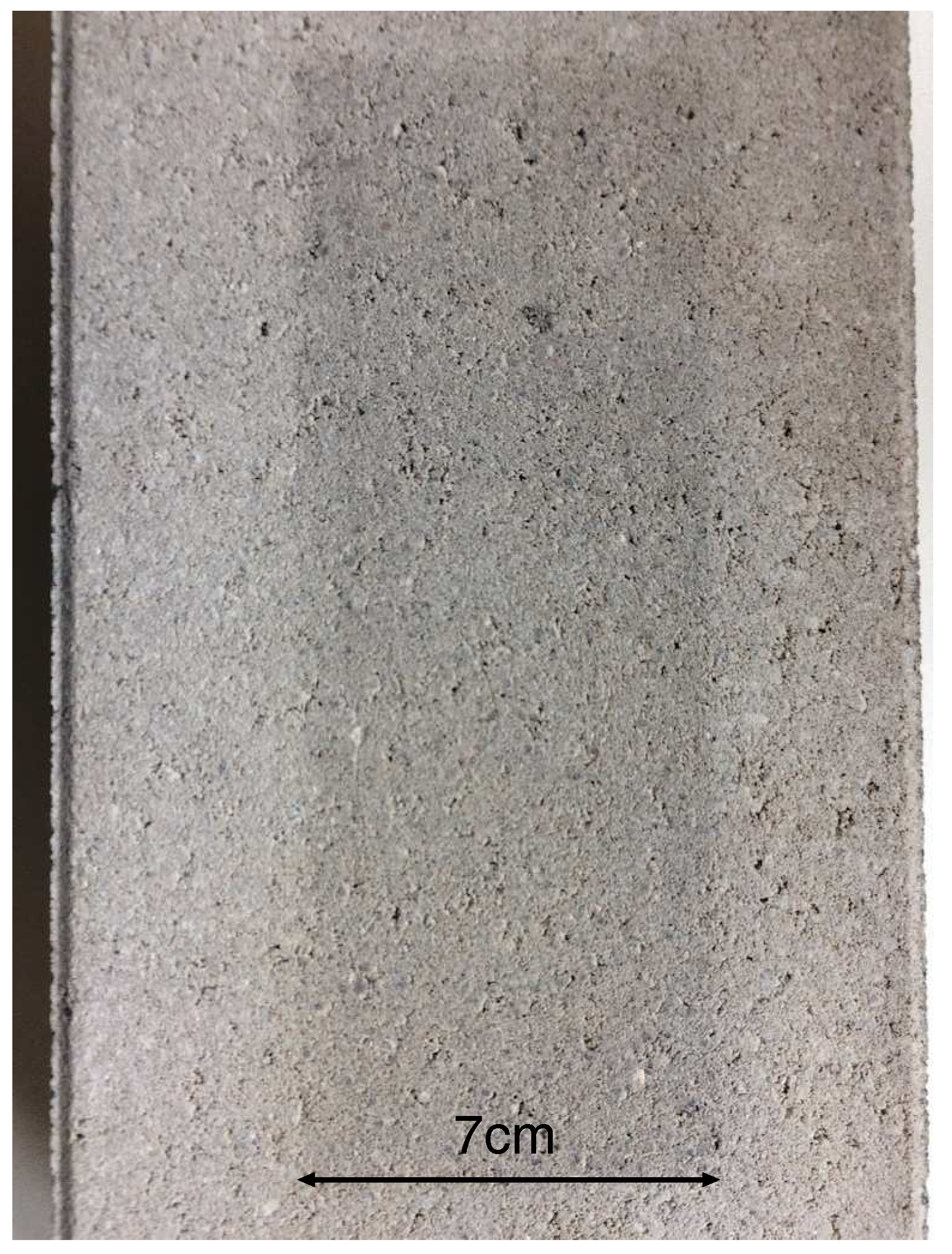
As substrates for the rubber friction studies, we have used smooth glass plates, concrete blocks, and an asphalt road track. The concrete blocks (see Figure 1) have been used in several earlier studies. They are very stable (negligible wear) and are easily available in a large number of nominally-identical blocks in a hardware store.
The most important information about rough surfaces is the surface roughness power spectrum. If we write the surface profile , given on a two-Dimensional (2D) square surface area, as the sum (or integral) of plane waves:
then the 2D power spectrum is defined as [8,10]:
where is the surface area. For surfaces with isotropic statistical properties, depends only on the magnitude of the wavevector . We can write , where is the wavelength of a surface roughness component.
Usually, we measure surface topography by line rather than by surface. From the line topography , one can calculate the 1D power spectrum. For surfaces with a roughness with isotropic statistical properties, all the information about surface roughness is already contained in the 1D line scan, and in this case, one can calculate the 2D power spectrum from the 1D power spectrum [11,12].
The glass surface can be considered as perfectly smooth. The surface roughness of the concrete and asphalt road surfaces was studied using a stylus instrument from Mitutoyo (Mitutoyo Portable Surface Roughness Measurement Surftest SJ-410) with a diamond tip having a radius of curvature m. The repulsive force between tip and substrate was , and we used the tip of speed m/s.
Figure 2 shows the 2D surface roughness power spectrum of the concrete surface (blue line). For the friction calculations, the surface roughness on the rubber surface is usually less important than for the counter-surface. However, in the adhesion study, the counter surface was a glass ball with a very smooth surface. In this case, the surface roughness of the rubber surface can be very important. This roughness is assumed to be determined by the surface roughness of the (steel) mold surface. In this study, we used two different steel molds: one with relatively large roughness and one with much smaller roughness. The power spectrum of the rough steel mold is shown in Figure 2 (green line).
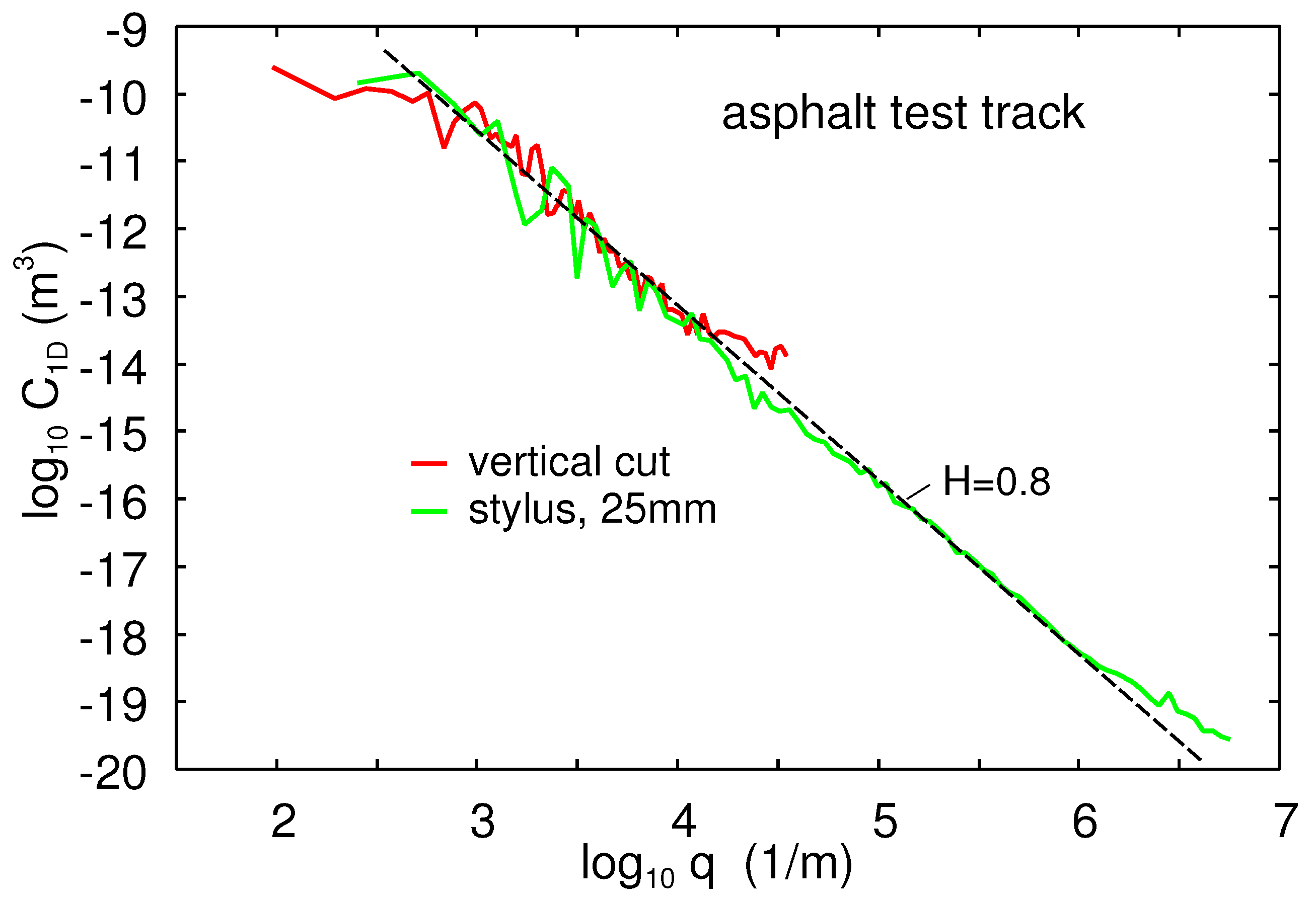
We have also measured the topography of the asphalt road test track used in some of the friction studies presented here with two different methods. The first method was direct measurements with the engineering stylus instrument. For the second method, we first produced a (and 1 cm thick) PDMS replica of the asphalt road surface. From this, we cut thin vertical slices and measured the topography using a scanner with a resolution of m (this method was also used on the concrete surface). This gives the long wavelength roughness power spectrum [13]. Figure 3 shows the obtained power spectrum. The red line is from the vertical cut of the PDMS replica. The green line is from engineering line scans on the PDMS replica. The red line corresponds to a surface with the rms roughness amplitude of . Note that both measurements give self-affine fractal power spectra with the Hurst exponent .
3. Viscoelastic Modulus
For rubber friction calculations, it is necessary to have information about the complex elastic modulus of the rubber over a rather large frequency range, as well as at different strain values including very large strain (of order one or 100% strain). The standard way of measuring the viscoelastic modulus is to deform the rubber sample in an oscillatory manner with a constant strain or stress amplitude. This is done at different frequencies and then repeated at different temperatures. The results measured at different temperatures can be shifted according to the time-temperature superposition principle to form a master curve covering a wide range of frequencies at the chosen reference temperature. This has been shown to be valid for unfilled polymers and is approximately true for filled rubber as well if the strain amplitude is small enough (below 0.001).
We have performed measurements of the viscoelastic modulus in both shear and in tensile (elongation) modes. The shear mode measurements give the shear modulus , while the measurements in tensile mode gives the Young’s modulus . These moduli are related via where is the Poisson ratio. Here, we will assume , which is accurate in the rubbery region, but less accurate in the glassy region. Hence, .
Figure 4 shows the real part of the Young’s modulus and the as a function of the logarithm of frequency. The measurements were performed in the tensile mode with a pre-strain of and with a dynamic strain amplitude of . The results at reference temperature are shown for the A (blue lines), B (red), and C (green) rubber compounds. The corresponding horizontal shift factors are shown in Figure 5.
We define the glass transition temperature as the temperature where is maximal, assuming the frequency . This definition gives the glass transition temperatures shown in Table 1. As expected, the winter compound has the lowest glass transition temperature.
When a rubber tread block is sliding on a road surface, the strain in asperity contact regions is typically very high, of order one. To take this into account, we performed strain sweep measurements up to a strain of order one. These measurements were carried out at different temperatures, but at a fixed frequency 10 Hz. The measured curves were shifted along the frequency axis using the shift factor obtained during construction of the viscoelastic master curve at low-strain. In this way, we can obtain an approximate “large-strain” master curve, which we use in the sliding friction calculations (see our accompanying paper in this volume of Lubricants about the non-linear viscoelastic modulus).
As an example, in Figure 6, we show the non-linear viscoelastic shear modulus G of Rubber Compounds A, B, and C, as a function of logarithm of the strain, obtained for the temperature and the frequency . Note that for the strain of order one, the real part of the modulus is about 10-times smaller than in the small-strain (linear response) region where the strain is <0.001. This has important implications for the rubber friction because the area of contact is roughly proportional to .
4. Adhesion
The contact region between a rigid spherical probe (radius R) and a flat rubber surface is circular with the radius r. In the JKR theory, the interaction between solids is described by the work of adhesion w, which is the energy per unit surface area to separate two flat surfaces from their equilibrium contact position to infinite separation. According to the JKR theory, the relation between interaction force F and the radius r on the stable branch of the interaction curve is [14,15]:
where , E and are the rubber Young’s modulus and Poisson ratio, respectively, and:
is the pull-off force. Thus, for an elastic solid, if the ball is pulled by a soft spring and neglecting the inertia effects, at , the pull-off force abruptly drops to zero. In the applications below, at equilibrium , the contact radius r = 0.1–1 mm.
The separation line can be considered as a crack tip [16,17]. The work of adhesion w in general depends on the velocity of the opening (during pull-off) or closing (during contact formation) crack tip. At finite crack tip velocity, for an opening crack, w can be strongly enhanced, and for a closing crack, strongly reduced, compared to the adiabatic (infinitely-low crack tip velocity) value .
Let us estimate the adiabatic work of adhesion between the rubber compound and the glass surface. The surface energy (per unit surface area) for glass cleaned with acetone and isopropanol (which result in a surface still covered by water and some (strongly-bonded) organic contamination) is typically 0.06–0.07 . The surface energy for rubber compounds is typically [18] 0.025–0.035 . In a simple approach, one assumes that the adiabatic work of adhesion is [19] , which in the present case gives 0.08–0.1 .
Interfacial crack propagation: The contact line between a spherical probe and a rubber substrate can be considered as a crack tip, and the work of adhesion w equals the crack propagation energy per unit surface area. It is known that the crack propagation energy depends on the crack tip velocity v and on the temperature T i.e., . In addition, it differs for a closing crack and an opening crack.
One contribution to the crack propagation energy (or work of adhesion) is derived from the viscoelastic energy dissipation in the vicinity of the crack tip (see Figure 7). For an opening crack, this will enhance w with a factor usually denoted as .
Here, we are interested in interfacial (between the glass ball and the rubber substrate) crack propagation. In this case, as the crack velocity (when viscous effects in the rubber are negligible), the measured value of can be identified as the energy needed to break the interfacial rubber-substrate bonds, which are usually of the van der Waals type.
The factor depends on the the viscoelastic energy dissipation inside the rubber close to the opening crack tip (red dashed region in Figure 7). It can be calculated from the measured viscoelastic modulus as described in [20,24].
For the three rubber compounds at C and at the crack tip velocity relevant for the study below, we get the viscoelastic enhancement factor (see Figure 8) (the factor of is derived from the fact that viscoelastic energy dissipation only occurs in one half space (in the rubber)).
Experimental set-up: We study the adhesion interaction between a spherical soda-lime glass ball (diameter ) and rubber. We bring the ball into contact with the substrate using a drive, which can be represented by a spring. The contact region is not observed directly, but only the time dependency of the interaction force is measured, from which we can calculate the crack tip velocity using (3).
The rubber substrate is positioned on a very accurate balance (analytical balance produced by Mettler Toledo, Model MS104TS/00), which has a reproducibility of (or ≈1 ) (see Figure 9). After zeroing the scale of the instrument, we can measure the force on the substrate as a function of time, which is directly transferred to a computer at a rate of 10 measurement points per second. To move the glass ball up and down, we use an electric motor coiling up a nylon cord, which is attached to the glass ball. The drive velocity as a function of time can be specified on a computer.
Most of our adhesion studies were performed on rubber surfaces prepared using the smooth steel mold. This is the same steel mold as was used in [26] (see Section 5.1 in [26]).
Experimental results: Figure 10 shows the interaction force between a glass ball and Rubber Compound A as a function of time. Results are shown in dry condition (red) and when immersed in water (green). The rubber surface was cleaned with hot water and the glass ball with acetone and isopropanol. The glass ball moved up and down with the vertical speed .
Figure 11 shows the work of adhesion between a glass ball and Rubber Compounds (with smooth surfaces) B, C, and A for dry contact and Figure 12 in water. The pull-off speed . Note that in the dry state, after several contacts, the work of adhesion is typically , which is the expected result if and the viscoelastic enhancement factor . In water, after several contacts, giving . Note that Compound B in water only exhibits adhesion during the first contact.
The rubber surfaces was cleaned with hot water before the experiments, and we believe that the reduction in adhesion with increasing time (see Figure 11 and Figure 12) is due to the migration of mobile molecules to the rubber surface. Alternatively, in each contact with the rubber surface, the glass ball picked up molecules from the rubber, which changed the adhesion during later contacts. That this indeed occurred, at least for the dry contact, will be shown below.
Figure 13 shows the interaction force between a glass ball and Rubber Compound B in water as a function of time.
We have performed some additional adhesion studies on rubber surfaces molded between the steel surfaces with higher surface roughness. In these cases, the magnitude of the work of adhesion (not shown) was similar to what we observed for the smoother rubber surfaces. This suggests that the surface roughness on both types of rubber surfaces has a relatively small influence on the pull-off force. This indicates that on the length scale given by the diameter of the JKR contact region (about 0.1–1 mm), the contact with the glass ball in the nominal contact area is complete and that the asperity deformation energy is small compared to the rubber-glass binding energy. We will now show optical microscopy images for the smooth rubber surface that support this conclusion.
5. Optical Pictures of the Rubber–Glass Contact
Using an optical microscope, we studied the contact between a smooth flat glass surface and rectangular rubber blocks of size and thickness . Figure 14 shows pictures for Rubber Compound B (smooth surface). The diameter of shown region is about . Before the experiments, the glass surface was cleaned with hot soapy water and the rubber surface with hot (≈90 ) destilled water. The surfaces were dried in the normal atmosphere for a few minutes, and the experiments were performed in the normal atmosphere.
The rectangular rubber block was first squeezed in contact with the glass with a very small nominal contact pressure (about ), after which the external pressure was removed. For dry contact, this resulted in what appeared (at the optical resolution of a few micrometer) to be complete contact except at some small defects (or contamination) regions. Next, an external force was applied to peel the rubber out of contact with the glass in half of the nominal rubber-glass contact region. Figure 14a shows a picture where the boundary line (crack edge) between contact (black region) and non-contact (gray region) is clearly seen. Note also the non-contact regions in the vicinity of defects inside the black (contact) region (one such region is indicated by the arrow). Such non-contact regions have been observed in the past as well for other rubber compounds [28].
In Figure 14b, we have added a small water droplet on the rubber surface before the rubber was squeezed in contact with the glass surface. Here, a thin water film separates the surfaces, resulting in the optical fringes seen in the picture. In this case, the rubber sheet could be moved laterally on the glass surface with a negligible lateral force. This is the expected result if a thin water film separates the surfaces.
6. Rubber Friction
6.1. Theory
There are two contributions to rubber friction force on rough surfaces. There is one contribution from the area of real contact and a viscoelastic contribution from the pulsating deformations it is exposed to during sliding from the substrate asperities. The contribution from the area of real contact can be directly probed on smooth surfaces. We write the friction force as:
If is the normal force, where is the nominal contact area and the nominal contact pressure, the friction coefficient:
where A is the area of real contact and the frictional shear stress in the area of contact. Here, we have also included a constant (velocity independent) friction coefficient , which may be due to the hard filler particles scratching the counter surface.
The Persson contact mechanics theory predict the viscoelastic contribution and the area of real contact A, but the dependency of frictional shear stress on velocity and temperature must be obtained using other theories or derived from experiments.
Viscoelastic contribution: In the theory of Persson, the friction force acting on a rubber block squeezed with the stress against a hard randomly rough surface is given by [29,30]:
where denotes the temperature and where:
where:
and:
where . Note that as , which is an exact result for complete contact. In fact, for complete contact, the expression (7) is exact. Note also that is the (normalized) contact area observed at the magnification .
Adhesive contribution: Let us consider the contribution from the area of real contact A to the friction force. For dry clean surfaces, we believe the most important friction processes are as follows: For sliding contact, the rubber molecules and the substrate atoms will interact as indicated in Figure 15. In many cases, one expects weak interfacial interactions, e.g., van der Waals interaction. For stationary contact, the rubber chains at the interface will adjust to the substrate potential to minimize the free energy. This bond formation may require overcoming potential barriers and will not occur instantaneously, but requires some relaxation time. During sliding at low velocity, thermal fluctuations will help to break the rubber–substrate bonds, resulting in a friction force that approaches zero as the sliding velocity goes to zero. At high velocity, there is not enough time for the rubber molecules to adjust to the substrate interaction potential, i.e., the bottom surface of the rubber block will “float” above the substrate, forming an incommensurate-like state with respect to the corrugated substrate potential. Thus, the frictional shear stress is small also for large sliding speed. We expect the frictional shear stress as a function of the sliding speed to have a maximum at some intermediate velocity . This friction mechanism was first studied in a highly-simplified model by Schallamach [31] and later by Leonov et al. [32], and for a more realistic model by Persson and Volokitin [33]. The theory predicts that the frictional shear stress is a Gaussian-like curve as a function of with a width of four (or more) frequency decades and centered at a sliding speed typically of order . This frictional shear stress law is very similar to what was observed (measured) by Grosch for rubber sliding on a smooth surfaces (glass or steel).
In [34], we found that using the following frictional shear stress law resulted in good agreement between theory and measurements:
where , 4–8 , and where the reference velocity for . The full width at half maximum of the as a function of is .
The master curve (11) is for the reference temperature , but the frictional shear stress at other temperatures can be obtained by replacing v with , where is the shift factor obtained when constructing the master curve (11). We have found that:
where the activation energy .
The contribution of the real contact area to rubber friction depends sensitively on the contamination particles and fluids. Thus, on a wet road surface at a high enough sliding (or rolling) speed, the surfaces in the apparent contact regions will be separated by a thin fluid film, in which case, the viscoelastic deformations of the rubber give the most important contribution to friction.
6.2. Experimental Section
We have performed rubber sliding friction experiments using three different friction testers. In addition, some vehicle braking distance measurements were performed, but these are less well defined experiments, as they depend on the Anti-lock Braking System (ABS) used and on the fact that the tire is rolling at finite slip in the vehicle experiments. In this case, the tread blocks perform a highly non-uniform sliding motion, with a negligible slip at the entrance of the tire-road footprint and a large slip close to the exit of the footprint. The observed tire-road friction force depends on the whole (time-dependent) interaction process between the tread blocks and the road surface.
Leonardo da Vinci experiment: The measured data were obtained using the setup shown in Figure 16. The slider consisted of two rubber blocks glued to a wood plate. One block was at the front and the other at the end of wood plate, and the nominal contact area . The normal force was generated by adding lead blocks (total mass M) on top of the wood plate. Similarly, the driving force was generated by adding lead blocks in the container in Figure 16.
The sliding distance as a function of time was measured using a distance sensor. This simple friction tester can be used for obtaining the friction coefficient as a function of sliding velocity and nominal contact pressure . Note that with this setup, the driving force was specified, and the velocity dependency of the friction can be studied only on the branch of the curve where the friction coefficient increased with increasing speed. In the Leonardo da Vinci experiments, the rubber blocks were run-in on the same substrates on which the measurements were performed.
Low temperature friction tester: In order to measure the friction coefficient also at lower temperatures, we have developed an experimental setup where the temperature can be changed from room temperature down to ; see Figure 17. A rectangular rubber block was glued into the milling grove of the sample holder, which became attached to the force cell (red box in the figure). The rubber specimen can move with the carriage in the vertical direction to adapt to the substrate profile. The normal load can simply be changed by adding additional steel weights on top of the force cell. The substrate sample became attached to the machine table, which was moved by a servo drive via a gearbox in a translational manner. Here, we controlled the relative velocity between the rubber specimen and the substrate sample, while the force cell acquired information about normal force, as well as friction force.
To change the temperature, the whole setup was placed inside a deep freezer capable of cooling down the experiment to . Then, we slid the rubber sample over the road surface with different velocities to gain information on the velocity dependency of the friction coefficient.
Linear friction tester: We have measured the friction coefficients for the sliding speeds of , , 1, and using a Linear Friction Tester (LFT). The LFT sample load was realized by adding additional weights on top of a plate with a rubber block, and in these tests, we used two loads, giving the nominal contact pressure of and .
Vehicle braking tests: Vehicle braking tests were performed for tires with tread blocks made from Tread Compounds A and B. The tests were performed on an asphalt road test track under dry and wet conditions. In the tests, a VW Golf car with ABS was used. From the measured braking distance, we calculated the effective friction coefficient assuming constant retardation.
6.3. Experimental Results
6.3.1. Sliding Friction on Dry and Wet Smooth Glass Surfaces
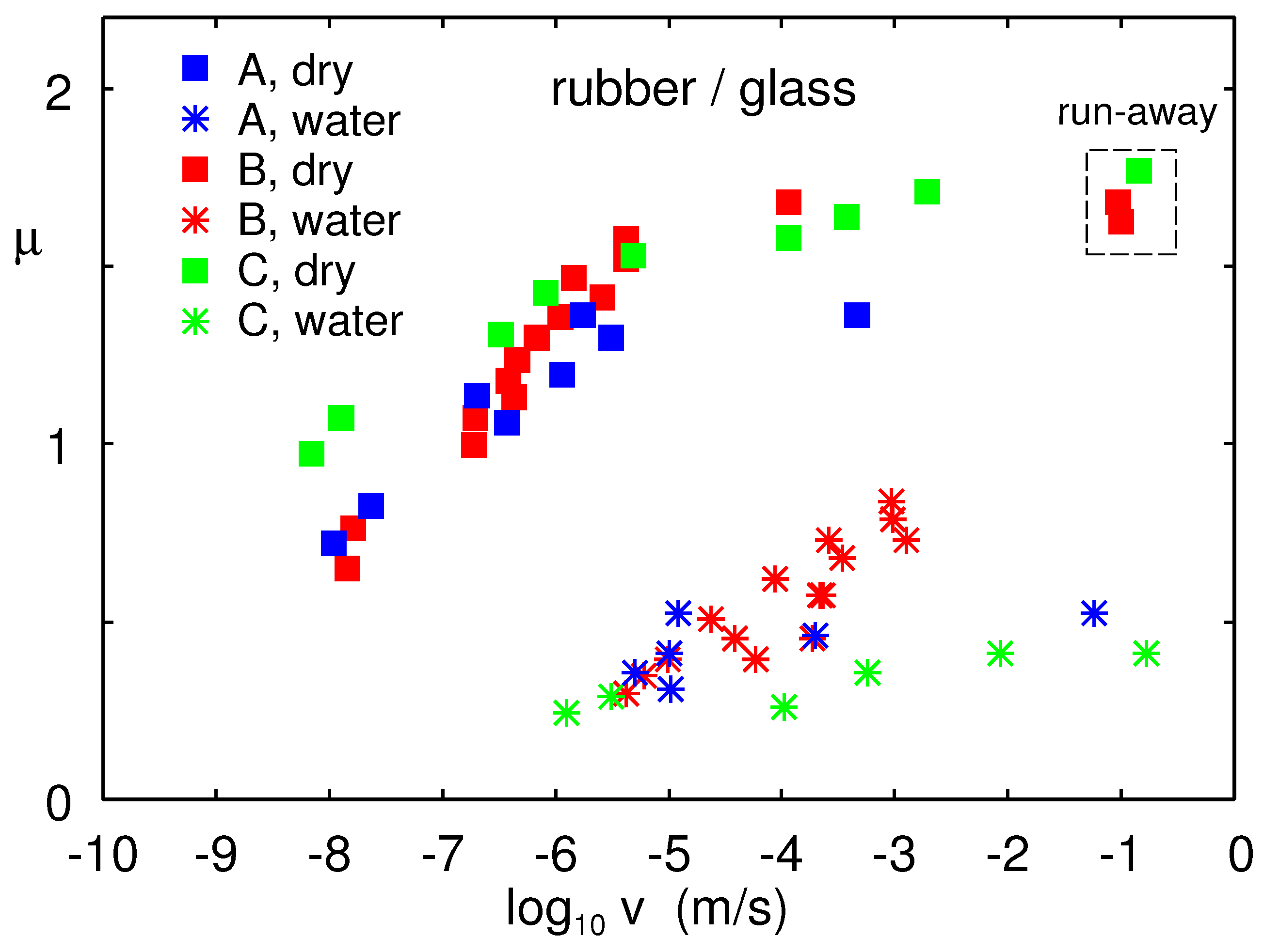
Figure 18 shows the friction coefficient for the dry rubber–glass contact (squares) and in water (stars) as a function of sliding speed for the B, C, and A rubber compounds. The temperature , and the nominal contact pressure . For low sliding speed (∼1 ) in water, the sliding friction force was about a factor of smaller than for the dry glass surface, which was similar to the reduction in the work of adhesion in Section 4 (compare Figure 11 to Figure 12).
One very important difference between sliding on a smooth and a rough substrate surface is illustrated in Figure 19. Here, we show the sliding distance as a function of time for Rubber Compound C on dry concrete (a) and on the dry glass surface (b). At time , the driving force was applied. For the rubber in contact with the concrete surface, most of the roughness was on the concrete surface, and the contact regions on the rubber were continuously changing position during sliding. This implies that the rubber-concrete contact area, and hence the sliding speed, did not change significantly in time.
For the rubber in contact with the (very smooth) glass surface, the same rubber asperities were in contact with the glass surface during sliding. In this case, because of viscoelastic relaxation and because of the time dependency of adhesion, the area of real contact increased with increasing time t, resulting in a sliding speed that decreased with time. That is, since the driving force was constant and since the frictional shear stress increased with increasing sliding speed (see Figure 18), in order for to stay constant, v must decrease with increasing contact time.
The complete study of the sliding dynamics of the rubber samples on dry and wet glass will be presented elsewhere.
6.3.2. Sliding Friction on Dry and Wet Concrete
We now present measured and calculated results for rubber sliding on concrete. The concrete surface had the power spectrum shown in Figure 20. The large and small wavenumber cut-off and used in the rubber friction calculations are indicated in the figure. The large wavenumber cut-off was chosen so that including all the roughness with wavenumber gave the rms slope of 1.3, as also used in earlier calculations.
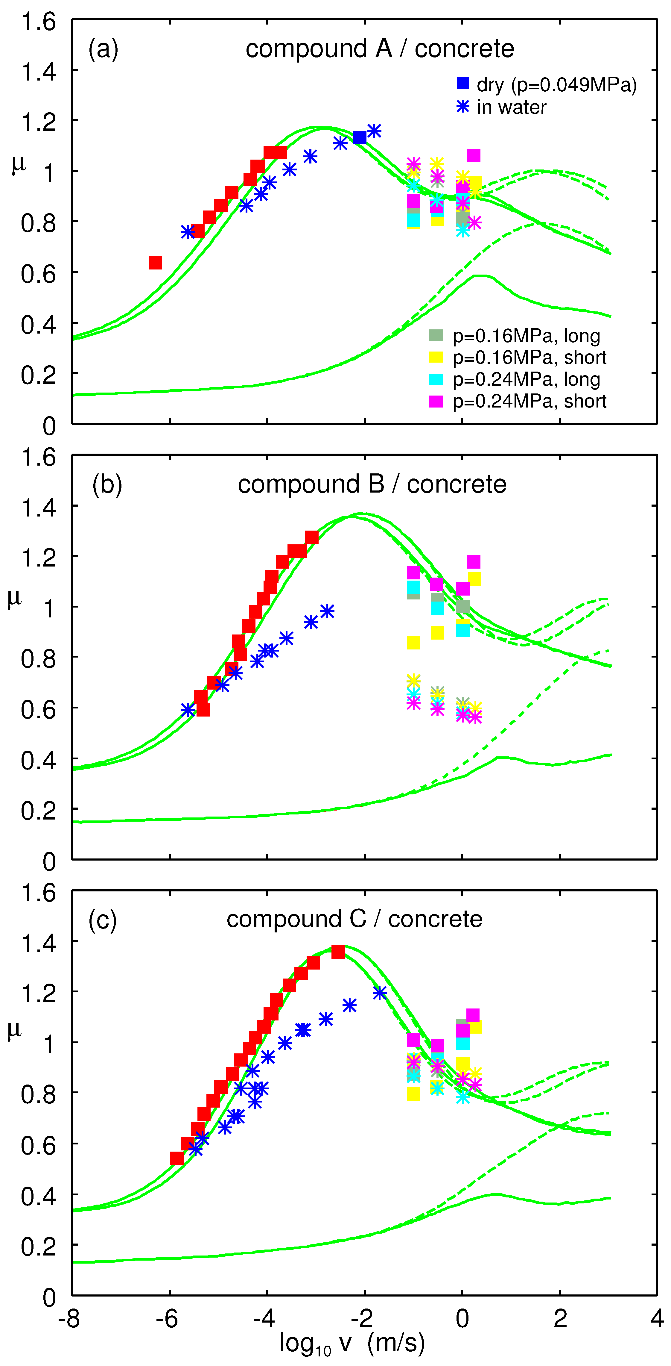
Figure 21 shows the measured and calculated friction coefficient on the concrete surface as a function of the logarithm of sliding speed. The measured data for low velocities (red squares and blue stars) was obtained using the Leonardo da Vinci setup, and the other higher velocity data were obtained using LFT. The square symbols are for dry surfaces and stars in water. The lower green curve is the (calculated) viscoelastic contribution to the friction coefficient, and the upper green curve the viscoelastic + adhesive contribution, plus a constant term , which may be attributed to scratching of the concrete surface by the hard filler particles. In each figure, there are two upper curves that are for the temperature prevailing in the Leonardo experiment () (curve to the left) and in LFT measurements () (curve to the right). The adhesive parameters used in the calculations are given in Table 2.
It is interesting to note that for the LFT measured friction, the higher nominal contact pressure appeared to give higher friction. This is in contrast to the behavior of tires where bigger normal load usually resulted in a lower effective friction coefficient. We attribute the latter to frictional heating (which is less important in the present experiments due to the shorter sliding distance) and to the change in tire footprint as the normal load increased [35].
It is very interesting to note that the high-velocity LFT friction coefficient in water correlates with the measured work of adhesion. Thus, Compound B in the water exhibited vanishing adhesion after some time in the water. Since adhesion between glass and rubber in water is associated with a dewetting transition and since dry rubber–road asperity contact regions are necessary for the adhesive contribution to the friction to prevail, it is expected that Rubber B will exhibit smaller friction than the other two compounds in water.
Note that Compounds A and C both exhibit about the same friction in the dry state and in water. Both of these compounds have resin additives, which is not the case for Compound B. One may ask if this is the reason for why the B compound in the LFT (high velocity) experiments exhibited much smaller friction in water than in the dry state!
6.3.3. Sliding Friction on Dry and Wet Asphalt Road
Friction experiments have also been performed on the asphalt test track. The experiments was performed using an LFT and also using a car with ABS.
The 1D power spectrum of the asphalt test track is given in Figure 3. The surface had the Hurst exponent , the rms roughness amplitude , and the roll-off wavenumber . The corresponding 2D power spectrum has been used in the theory calculations presented below.
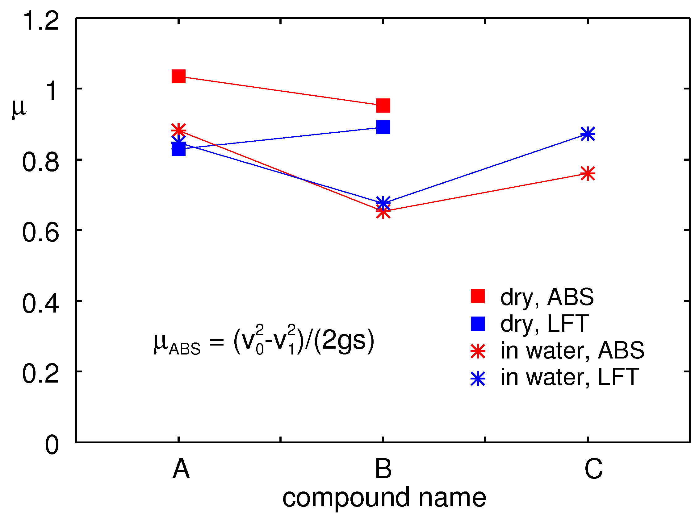
Figure 22 shows the measured friction coefficient on the asphalt test track obtained using the LFT at the sliding speed and also the results obtained using the VW Golf car with ABS braking. In the latter case, the friction coefficient was calculated from the distance s needed to reduce the car velocity from to using:
where is the gravitational constant. The square symbols are for dry surfaces and the stars in water.
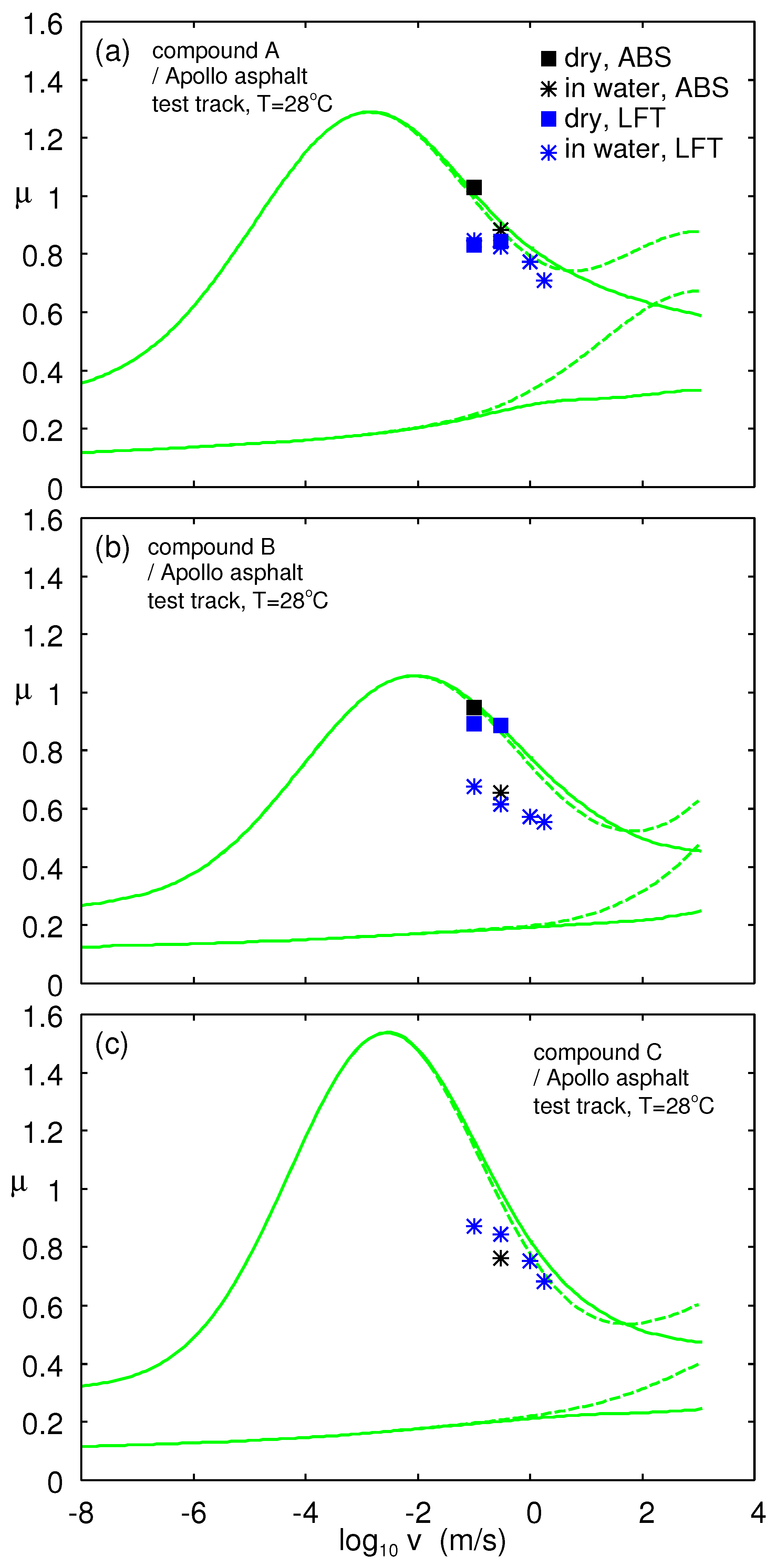
In Figure 23, we show the measured (symbols) and calculated (lines) friction coefficient on the asphalt track as a function of the logarithm of sliding speed. The measured data were obtained using the LFT. Square symbols are for dry surfaces and stars in water. The lower calculated curves is the viscoelastic contribution to the friction coefficient and the upper the viscoelastic + adhesive contributions plus a constant term , which we attributed to scratching of the concrete surface by the hard filler particles. The temperature prevailing in the LFT experiments and the vehicle tests in the dry condition was . In the vehicle experiments in water, . The theory results (green curves) are for . The adhesive parameters are given in Table 2 except for Compound B, where we used . The friction coefficient was obtained from the vehicle braking distance s using (13). For the vehicle friction, the tread block slip velocity depends on time, and in the figure, we assumed the effective (say time-averaged) slip velocity in water and in the dry state. In reality, the tread blocks undergoes non-uniform slip dynamics, where the slip velocity is close to zero when a tread block enters the tire–road footprint, while the slip velocity typically is of the order pf a few m/s when the tread block leaves the footprint.
6.3.4. Low Temperature Experiments for Compound C on Concrete
Figure 24 shows the friction coefficient as a function of the logarithm of sliding speed for the C rubber compound, for several temperatures. The green lines are the theory predictions. The lower green lines are the viscoelastic contribution to the friction and the upper green lines the viscoelastic contribution plus the contribution from the area of real contact.
In this study, the parameters that determine the adhesive contribution to the friction were optimized at and then used in the calculation of friction for the other temperatures. There was good quantitatively agreement between theory and experiments, but we note here that sliding the rubber block in the forward and backward direction on the concrete surface gave different results. We have observed this in the past as well, and sometimes, the friction differed by 30–40% between the two sliding directions, in spite of the fact that visual inspection of the rubber block did not indicate any asymmetry between the two sliding directions [36]. In fact, the friction coefficients obtained above (at ) were ≈40% smaller than found with the Leonardo da Vinci setup.
6.3.5. Influence of Rubber Transfer (Smear) to the Road Surface on the Sliding Friction
It is known from F1-racing that the transfer of rubber to the racing track can have a strong influence on the sliding friction or grip. In particular, when changing to new tires with a different rubber tread compound, the friction can be reduced compared to a clean road surface. We have tested this on our concrete surface. Figure 25 shows the friction coefficient as a function of the logarithm of sliding speed for the A rubber compound at . Measurements was performed in the low temperature linear friction tester on a new concrete surface (red) and on a concrete surface on which measurements with another rubber compound were already done. Note the big drop in the friction. More studies are needed to confirm this result and show how general this effect may be.
7. Summary and Conclusions
We have studied the adhesion and friction for three tire tread rubber compounds. The linear and non-linear viscoelastic properties of the rubber compounds were measured in shear and in tension mode using two different Dynamic Mechanical Analysis (DMA) instruments. The surface topography of all surfaces was determined using stylus measurements and scanned-in silicon rubber replicas.
In the adhesion studies, a smooth silica glass ball was brought repeatedly in contact with smooth sheets of the rubber in dry condition and in water. We found that one of the compounds exhibited adhesion in water only for a short time. The same rubber compound exhibited smaller sliding friction in water than the other two compounds, which exhibited adhesion in water also after a long time.
Friction studies were performed for rubber sliding on smooth glass, concrete, and asphalt road surfaces, using the Leonardo da Vinci-type of friction experiments and experiments using a linear friction tester. On the asphalt road, we also performed vehicle breaking distance measurements. The measured friction coefficients was found to be in good agreement with the Persson contact mechanics theory predictions. The results show the importance of the contribution to the friction coefficient from the area of real contact (the adhesive contribution). This contribution exhibited a maximum at low sliding speed (0.1–1 cm/s), and with respect to ABS tire dynamics, it will act as an effective static friction coefficient, which determined the boundary line in the tire-road footprint between thread blocks (on the entrance side), which does not slip (or slip with very low speed), and tread blocks (on the exit side), which slip fast (speed of order ∼1–10 m/s). Hence, the adhesive contribution to the friction will have a strong influence on the position and the maximum of the tire -slip curve.
One very important difference between the sliding on smooth and rough substrate surface was illustrated in our study with a rubber block sliding on a concrete surface and a smooth glass surface. For the rubber in contact with the concrete surface, most of the roughness was on the concrete surface, and the contact regions on the rubber were continuously changing position during sliding. This implies that the rubber–concrete contact area, and hence the sliding speed, does not change significantly with time.
For the rubber in contact with the smooth glass surface, the same rubber asperities were in contact with the glass surface during sliding. In this case, because of viscoelastic relaxation and because of the time dependency of adhesion, the area of real contact increased with increasing time, resulting in a sliding speed, which decreased with time.
Author Contributions
Both authors have contributed equally to this paper.
Acknowledgments
We thank Avinash Tiwari for help with the DMA measurements. This work was performed within a Reinhart-Koselleck project funded by the Deutsche Forschungsgemeinschaft (DFG). B.N.J.P. would like to thank DFG for the project support under the reference German Research Foundation DFG-Grant MU 1225/36-1. B.N.J.P. also acknowledges supported by the DFG-Grant PE 807/12-1.
Conflicts of Interest
There are no conflict of interest.
References
- Persson, B.N.J. Sliding Friction: Physical Principles and Applications; Springer: Heidelberg, Germany, 2000. [Google Scholar]
- Gnecco, E.; Meyer, E. Elements of Friction Theory and Nanotribology; Cambridge University Press: Cambridge, UK, 2015. [Google Scholar]
- Israelachvili, J.N. Intermolecular and Surface Forces, 3rd ed.; Academic: London, UK, 2011. [Google Scholar]
- Barber, J.R. Contact Mechanics (Solid Mechanics and Its Applications); Springer: Berlin/Heidelberg, Germany, 2018. [Google Scholar]
- Persson, B.N.J. Contact Mechanics for Randomly Rough Surfaces. Surf. Sci. Rep. 2006, 61, 201–227. [Google Scholar] [CrossRef]
- Heinrich, G.; Klüppel, M. Recent Advances in the Theory of Filler Networking in Elastomers; Advances in Polymer Science; Springer-Verlag: Berlin/Heidelberg, Germany, 2002; Volume 160. [Google Scholar]
- Heinrich, G.; Vilgis, T.A. A statistical mechanical approach to the Payne effect in filled rubbers. Express Polym. Lett. 2015, 9, 291. [Google Scholar] [CrossRef]
- Persson, B.N.J. On the fractal dimension of rough surfaces. Tribol. Lett. 2014, 54, 99–106. [Google Scholar] [CrossRef]
- Tiwari, A.; Miyashita, N.; Espallargas, N.; Persson, B.N.J. Rubber friction: The contribution from the area of real contact. J. Chem. Phys. 2018, 148, 224701. [Google Scholar] [CrossRef] [PubMed]
- Persson, B.N.J.; Albohr, O.; Tartaglino, U.; Volokitin, A.I.; Tosatti, E. On the nature of surface roughness with application to contact mechanics, sealing, rubber friction and adhesion. J. Phys. Condens. Matter 2005, 17, R1. [Google Scholar] [CrossRef] [PubMed]
- Nayak, P.R. Random process model of rough surfaces. J. Lubr. Technol. 1971, 93, 398–407. [Google Scholar] [CrossRef]
- Carbone, G.; Lorenz, B.; Persson, B.N.J.; Wohlers, A. Contact mechanics and rubber friction for randomly rough surfaces with anisotropic statistical properties. Eur. Phys. J. E 2009, 29, 275–284. [Google Scholar] [CrossRef] [PubMed]
- Persson, J.S.; Tiwari, A.; Valbahs, E.; Tolpekina, T.V.; Persson, B.N.J. On the Use of Silicon Rubber Replica for Surface Topography Studies. Tribol. Lett. 2018, 66, 140. [Google Scholar] [CrossRef]
- Johnson, K.L.; Kendall, K.; Roberts, A.D. Surface energy and the contact of elastic solids. Proc. R. Soc. Lond. A 1971, 324, 301. [Google Scholar] [CrossRef]
- Deruelle, M.; Hervet, H.; Jandeau, G.; Leger, L. Some remarks on JKR experiments. J. Adhes. Sci. Technol. 1998, 12, 225–247. [Google Scholar] [CrossRef]
- Greenwood, J.A.; Johnson, K.L. The mechanics of adhesion of viscoelastic solids. Philos. Mag. 1981, 43, 697–711. [Google Scholar] [CrossRef]
- Maugis, D.; Barquins, M. Fracture mechanics and the adherence of viscoelastic bodies. J. Appl. Phys. D 1978, 11, 1989. [Google Scholar] [CrossRef]
- Available online: www.accudynetest.com/polymer_surface_data/butyl_rubber.pdf (accessed on 26 February 2019).
- Manoj, K.; Chaudhury, M.K. Interfacial interaction between low-energy surfaces. Mater. Sci. Eng. 1996, R16, 97–159. [Google Scholar]
- Persson, B.N.J.; Brener, E.A. Crack propagation in viscoelastic solids. Phys. Rev. E 2005, 71, 036123. [Google Scholar] [CrossRef] [PubMed]
- Greenwood, J.A. The theory of viscoelastic crack propagation and healing. J. Phys. D Appl. Phys. 2004, 37, 2557. [Google Scholar] [CrossRef]
- Greenwood, J.A. Viscoelastic crack propagation and closing with Lennard-Jones surface forces. J. Phys. D Appl. Phys. 2007, 40, 1769. [Google Scholar] [CrossRef]
- Mueller, H.K.; Knauss, W.G. Crack Propagation in a Linearly Viscoelastic Strip. J. Appl. Mech. 1971, 38, 483–488. [Google Scholar] [CrossRef]
- Persson, B.N.J.; Albohr, O.; Heinrich, G.; Ueba, H. Crack propagation in rubber-like materials. J. Phys. Condens. Matter 2005, 17, R1071. [Google Scholar] [CrossRef]
- Carbone, G.; Persson, B.N.J. Hot Cracks in Rubber: Origin of the Giant Toughness of Rubberlike Materials. Phys. Rev. Lett. 2005, 95, 114301. [Google Scholar] [CrossRef] [PubMed]
- Tiwari, A.; Dorogin, L.; Bennett, A.I.; Schulze, K.D.; Sawyer, W.G.; Tahir, M.; Heinrich, G.; Persson, B.N.J. The effect of surface roughness and viscoelasticity on rubber adhesion. Soft Matter 2017, 13, 3602–3621. [Google Scholar] [CrossRef] [PubMed]
- Tiwari, A.; Dorogin, L.; Tahir, M.; Stöckelhuber, K.W.; Heinrich, G.; Espallargas, N.; Persson, B.N. Rubber contact mechanics: Adhesion, friction and leakage of seals. Soft Matter 2017, 13, 9103–9121. [Google Scholar] [CrossRef] [PubMed]
- Lorenz, B.; Krick, B.A.; Mulakaluri, N.; Smolyakova, M.; Dieluweit, S.; Sawyer, W.G.; Persson, B.N.J. Adhesion: Role of bulk viscoelasticity and surface roughness. J. Phys. Condens. Matter 2013, 25, 225004. [Google Scholar] [CrossRef] [PubMed]
- Persson, B.N.J. Theory of rubber friction and contact mechanics. J. Chem. Phys. 2001, 115, 3840–3861. [Google Scholar] [CrossRef]
- Scaraggi, M.; Persson, B.N.J. Friction and universal contact area law for randomly rough viscoelastic contacts. J. Phys. Condens. Matter 2015, 27, 105102. [Google Scholar] [CrossRef] [PubMed]
- Schallamach, A. A theory of dynamic rubber friction. Wear 1963, 6, 375–382. [Google Scholar] [CrossRef]
- Cherniak, Y.B.; Leonov, A.I. On the theory of the adhesive friction of elastomers. Wear 1986, 108, 105–138. [Google Scholar] [CrossRef]
- Persson, B.N.J.; Volokitin, A.I. Rubber friction on smooth surfaces. Eur. Phys. J. E 2006, 21, 69–80. [Google Scholar] [CrossRef] [PubMed]
- Lorenz, B.; Oh, Y.R.; Nam, S.K.; Jeon, S.H.; Persson, B.N.J. Rubber friction on road surfaces: Experiment and theory for low sliding speeds. J. Chem. Phys. 2015, 142, 194701. [Google Scholar] [CrossRef] [PubMed]
- Persson, B.N.J. Rubber friction and tire dynamics. J. Phys. Condens. Matter 2010, 23, 015003. [Google Scholar] [CrossRef] [PubMed]
- Tiwari, A.; Dorogin, L.; Steenwyk, B.; Warhadpande, A.; Motamedi, M.; Fortunato, G.; Ciaravola, V.; Persson, B.N.J. Rubber friction directional asymmetry. Europhys. Lett. 2017, 116, 66002. [Google Scholar] [CrossRef]
Figure 1.
The concrete surface used in some of the experiments. The dark region arose from transfer of rubber material to the concrete surface during sliding at for two cycles (each cycle is ) at . Reproduced from [9], with the permission of AIP Publishing, 2018.
Figure 1.
The concrete surface used in some of the experiments. The dark region arose from transfer of rubber material to the concrete surface during sliding at for two cycles (each cycle is ) at . Reproduced from [9], with the permission of AIP Publishing, 2018.

Figure 2.
The 2D surface roughness power spectrum of the concrete and (rough) steel mold surfaces used in this study.
Figure 2.
The 2D surface roughness power spectrum of the concrete and (rough) steel mold surfaces used in this study.

Figure 3.
The 1D power spectrum of the asphalt road test track. The red line is from the PDMS replica. The green line is from stylus line scans. The red line corresponds to a surface with the rms roughness amplitude of .
Figure 3.
The 1D power spectrum of the asphalt road test track. The red line is from the PDMS replica. The green line is from stylus line scans. The red line corresponds to a surface with the rms roughness amplitude of .

Figure 4.
The real part of the Young’s modulus (a) and the (b) as a function of the logarithm of frequency. For the A, B, and C rubber compounds at the reference temperature obtained from low-strain measurements ( dynamical strain amplitude and pre-strain).
Figure 4.
The real part of the Young’s modulus (a) and the (b) as a function of the logarithm of frequency. For the A, B, and C rubber compounds at the reference temperature obtained from low-strain measurements ( dynamical strain amplitude and pre-strain).

Figure 5.
The logarithm of temperature-frequency shift factor as a function of temperature for Rubber Compounds A, B, and C. For the reference temperature .
Figure 5.
The logarithm of temperature-frequency shift factor as a function of temperature for Rubber Compounds A, B, and C. For the reference temperature .

Figure 6.
The real part (a) and the imaginary part (b) of the shear modulus G of Rubber Compounds A, B, and C as a function of the logarithm of the strain. For the temperature and the frequency .
Figure 6.
The real part (a) and the imaginary part (b) of the shear modulus G of Rubber Compounds A, B, and C as a function of the logarithm of the strain. For the temperature and the frequency .

Figure 7.
A rigid ball pulled away from a viscoelastic solid. A part of the energy needed to remove the ball is derived from the viscoelastic energy dissipation inside the rubber close to the opening crack tip (red dashed region).
Figure 7.
A rigid ball pulled away from a viscoelastic solid. A part of the energy needed to remove the ball is derived from the viscoelastic energy dissipation inside the rubber close to the opening crack tip (red dashed region).

Figure 8.
Viscoelastic contribution to the crack propagation energy as a function of the crack speed (log-log scale), at the temperature , calculated using the bulk viscoelastic modulus. The vertical line is the crack tip speeds for the pull-off in the adhesion experiments.
Figure 8.
Viscoelastic contribution to the crack propagation energy as a function of the crack speed (log-log scale), at the temperature , calculated using the bulk viscoelastic modulus. The vertical line is the crack tip speeds for the pull-off in the adhesion experiments.

Figure 9.
The experimental setup for measuring adhesion [27].
Figure 9.
The experimental setup for measuring adhesion [27].

Figure 10.
The interaction force between a glass ball and Rubber Compound A as a function of time. Results are shown in the dry condition (red) and when immersed in water (green). The rubber surface was cleaned with hot water and the glass ball with acetone and isopropanol. The glass ball moved up and down with the vertical speed .

Figure 11.
The work of adhesion between a glass ball and Rubber Compounds B, C, and A with very smooth surfaces for dry contact. The pull-off speed .
Figure 11.
The work of adhesion between a glass ball and Rubber Compounds B, C, and A with very smooth surfaces for dry contact. The pull-off speed .

Figure 12.
The work of adhesion between a glass ball and Rubber compounds B, C, and A with very smooth surfaces in water. The pull-off speed .
Figure 12.
The work of adhesion between a glass ball and Rubber compounds B, C, and A with very smooth surfaces in water. The pull-off speed .

Figure 13.
The interaction force between a glass ball and Rubber Compound B in water as a function of time. The rubber surface was cleaned with hot water and the glass ball with acetone and isopropanol. The glass ball moved up and down with the vertical speed .
Figure 13.
The interaction force between a glass ball and Rubber Compound B in water as a function of time. The rubber surface was cleaned with hot water and the glass ball with acetone and isopropanol. The glass ball moved up and down with the vertical speed .

Figure 14.
(a) Optical picture of the dry contact between a flat glass surface and the smooth Rubber B’s surface. An external force was applied to peel the rubber out of contact with the glass in half of the nominal rubber-glass contact region. (b) A small water droplet was deposited on the rubber surface before the rubber was squeezed in contact with the glass surface. A thin water film separates the surfaces, resulting in the optical fringes seen in the picture. (c) After contact in the dry state, a thin contamination film was deposited on the glass surface. The diameter of pictures is about . The white elliptic regions in the figures are due to the eight light diodes used to illuminate the contact.

Figure 15.
The classical description of a polymer chain at the rubber–block counter surface interface. During lateral motion of the rubber block, a chain stretches, detaches, relaxes, and reattaches to the surface to repeat the cycle. The picture is schematic, and in reality, no detachment in the vertical direction is expected, but only a rearrangement of molecule segments (in nanometer-sized domains) parallel to the surface from pinned (commensurate-like) to depinned (incommensurate-like) domains, [27].

Figure 16.
Simple friction tester (schematic) used for obtaining the friction coefficient as a function of the sliding speed. The sliding distance is measured using a distance sensor and the sliding velocity obtained by dividing the sliding distance with the sliding time. This setup can only measure the friction coefficient on the branch of the -curve where the friction coefficient increases with increasing sliding speed v,27].

Figure 17.
Schematic picture of the low-temperature friction instrument allowing for linear reciprocal motion. Reproduced from [9], with the permission of AIP Publishing, 2018.
Figure 17.
Schematic picture of the low-temperature friction instrument allowing for linear reciprocal motion. Reproduced from [9], with the permission of AIP Publishing, 2018.

Figure 18.
The friction coefficient for the dry rubber-glass contact (squares) and in water (stars) as a function of the sliding speed. For the temperature and the nominal contact pressure .
Figure 18.
The friction coefficient for the dry rubber-glass contact (squares) and in water (stars) as a function of the sliding speed. For the temperature and the nominal contact pressure .

Figure 19.
The sliding distance as a function of time for Rubber Compound C on dry concrete (a) and on dry borosilicate glass (b). At time , the driving force is applied where (green line) and (red line) in case (a) and (green line) and (red line) in case (b). The normal load corresponding to the nominal contact pressure .

Figure 20.
The surface roughness power spectrum of the concrete used in this study. For the concrete surface, we used the large wavenumber cut-off or cut-off length .
Figure 20.
The surface roughness power spectrum of the concrete used in this study. For the concrete surface, we used the large wavenumber cut-off or cut-off length .

Figure 21.
The measured (symbols) and calculated (green lines) friction coefficient on concrete as a function of the logarithm of the sliding speed for Compound A (a), B (b) and C (c). The measured data for low velocities were obtained using the Leonardo da Vinci setup, and the other data were obtained using a Linear Friction Tester (LFT). The square symbols are for dry surfaces and stars in water. The lower calculated curves are the viscoelastic contribution to the friction coefficient and the upper the viscoelastic + adhesive contribution plus a constant term , which we attribute to scratching of the concrete surface by the hard filler particles. In each figure, there are two upper curves that are for the temperature prevailing in the Leonardo experiment () (curve to the left) and in the linear friction tester () (curve to the right). The adhesive parameters are given in Table 2.

Figure 22.
The measured friction coefficient on the asphalt test track obtained using LFT at the sliding speed and using the VW Golf car with ABS braking. In the latter case, the friction coefficient was calculated from the distance s. The square symbols are for dry surfaces and the star in water. For Rubber Compounds A, B, and C.

Figure 23.
The measured (symbols) and calculated (lines) friction coefficient on concrete as a function of the logarithm of the sliding speed for Compound A (a), B (b) and C (c). The measured data were obtained using the LFT. Square symbols are for dry surfaces and stars in water. The black symbols are the calculated (see the text) effective friction coefficients obtained from the vehicle braking distance, where we have assumed the average slip velocities in water (stars) and for dry surface (squares). The lower solid (green) curve is the viscoelastic contribution to the friction coefficient and the upper the viscoelastic + adhesive contribution plus a constant term , which we attribute to scratching of the concrete surface by the hard filler particles. The temperature prevailing in the LFT experiments and the vehicle tests in the dry condition is . In the vehicle experiments in water, . The theory results (green curves) are for . The adhesive parameters are given in Table 2, except for Compound B, where we used .

Figure 24.
The friction coefficient as a function of the logarithm of sliding speed for the C rubber compound, for several temperatures. The results were from the low-temperature linear friction tester. The green lines are the theory predictions. The lower green lines are the viscoelastic contribution to the friction and the upper green lines the viscoelastic contribution plus the contribution from the area of real contact.

Figure 25.
The friction coefficient as a function of the logarithm of sliding speed for the A compound at . Measurements were performed on a new concrete surface (red) and on a concrete surface on which measurements with another rubber compound were already done.
Figure 25.
The friction coefficient as a function of the logarithm of sliding speed for the A compound at . Measurements were performed on a new concrete surface (red) and on a concrete surface on which measurements with another rubber compound were already done.


Table 1.
Summary of the glass transition temperatures of the A, B, and C compounds. The glass transition temperature is defined as the maximum of tan as a function of temperature for the frequency .
Table 1.
Summary of the glass transition temperatures of the A, B, and C compounds. The glass transition temperature is defined as the maximum of tan as a function of temperature for the frequency .
| Compound | Maximum of tan | |
|---|---|---|
| A | 0.53 | |
| B | 0.52 | |
| C | 0.41 |
Table 2.
Summary of adhesion parameters.
| Compound | (MPa) | (m/s) | ||
|---|---|---|---|---|
| A | 4.9 | −2.47 | 0.2 | |
| B | 4.7 | −1.97 | 0.2 | |
| C | 4.1 | −2.53 | 0.2 |
© 2019 by the authors. Licensee MDPI, Basel, Switzerland. This article is an open access article distributed under the terms and conditions of the Creative Commons Attribution (CC BY) license (http://creativecommons.org/licenses/by/4.0/).
Share and Cite
MDPI and ACS Style
Tolpekina, T.V.; Persson, B.N.J. Adhesion and Friction for Three Tire Tread Compounds. Lubricants 2019, 7, 20. https://doi.org/10.3390/lubricants7030020
AMA Style
Tolpekina TV, Persson BNJ. Adhesion and Friction for Three Tire Tread Compounds. Lubricants. 2019; 7(3):20. https://doi.org/10.3390/lubricants7030020
Chicago/Turabian StyleTolpekina, T. V., and B. N. J. Persson. 2019. "Adhesion and Friction for Three Tire Tread Compounds" Lubricants 7, no. 3: 20. https://doi.org/10.3390/lubricants7030020
Note that from the first issue of 2016, this journal uses article numbers instead of page numbers. See further details here.