The Influence of Test-Panel Orientation and Exposure Angle on the Corrosion Rate of Carbon Steel. Mathematical Modelling


1
Department of Process Engineering, University of Las Palmas de Gran Canaria, 35017 Las Palmas de Gran Canaria, Gran Canaria, Canary Islands, Spain
2
Department of Applied Economics and Quantitative Methods, University of La Laguna, 38071 La Laguna, Tenerife, Spain
3
Faculty of Sciences and Technology, Azores University, 9500-321 Ponta Delgada, São Miguel, Azores Islands, Portugal
4
Centre of Physics and Technological Research (CEFITEC), Faculty of Sciences and Technology, Universidade Nova de Lisboa, 2829-516 Caparica, Portugal
5
Centre of Biotechnology of Azores (CBA), 9500-321 Ponta Delgada, São Miguel, Azores Islands, Portugal
6
Department of Chemistry, University of La Laguna, 38200 La Laguna, Tenerife, Canary Islands, Spain
7
Institute of Material Science and Nanotechnology, University of La Laguna, 38200 La Laguna, Tenerife, Canary Islands, Spain
*
Author to whom correspondence should be addressed.
Metals 2020, 10(2), 196; https://doi.org/10.3390/met10020196
Submission received: 29 December 2019
/
Revised: 23 January 2020
/
Accepted: 27 January 2020
/
Published: 29 January 2020
(This article belongs to the Special Issue Corrosion and Protection of Metals)
Abstract
:The effects of both test-panel orientation and exposure angle on the atmospheric corrosion rates of carbon steel probes exposed to a marine atmosphere were investigated. Test samples were exposed in a tree-shape metallic frame with either three exposure angles of 30°, 45° and 60° and orientation north-northeast (N-NE), or eight different orientation angles around a circumference. It was found that the experimental corrosion rates of carbon steel decreased for the specimens exposed with greater exposure angles, whereas the highest corrosion rates were found for those oriented to N-NE due to the influence of the prevailing winds. The obtained data obtained were fitted using the bi-logarithmic law and its variations as to take in account the amounts of pollutants and the time of wetness (TOW) for each particular case with somewhat good agreement, although these models failed when all the effects were considered simultaneously. In this work, we propose a new mathematical model including qualitative variables to account for the effects of both exposure and orientation angles while producing the highest quality fits. The goodness of the fit was used to determine the performance of the mathematical models.
1. Introduction
Corrosion prevention is an essential task in many areas of society, especially in engineering applications where metals or metal alloys are used [1,2]. Many industries are often faced with serious economic consequences due to unexpected component failures when regular maintenance was not foreseen. In particular, the damage caused by atmospheric corrosion accounts for more than half of the total cost caused by the corrosion phenomena [1,3,4]. Metals are consumed by electrochemical reactions which rates depend on the exposure time (TEXP) but the phenomenon itself is very complex since is also highly dependent on numerous damage factors [4,5,6,7], each of which are extremely variable. These factors include natural air pollutants and anthropogenic sources [4,5], mainly sulfur dioxide (SO2), salinity (chlorides, CL) and other pollutants, such as ‘particulate matter’ or ‘PM’, as well as climatic factors such as relative humidity, time of wetness (TOW), temperature, rainfall and wind speed, but also physical characteristics such as shape and type of metal (ferrous or non-ferrous) [4,8], exposure angle [9,10], orientation [8,9,10,11,12] and geographic location [4].
The effects of the atmosphere on the corrosion rate are generally studied by exposing metallic samples to the environment. Then, when both corrosion rate and the environmental parameters are properly measured, relationships between the various damage factors are established through mathematical models [13,14,15,16,17,18,19,20,21]. The goodness of a fit has been employed to compare the theoretical model to observed data. These tools have become essential for corrosion prevention because they allow forecasting metal behavior in potentially corrosive real operating situations. For example, carbon steel undergoes a less severe attack in urban environments (C3) than in marine environments (C5) [10,22,23].
Many of these models address the combination of climate and air pollutant variables and their influence on the corrosion rate in order to estimate the loss of thickness or the loss of mass per unit area of metallic material. A very popular approach to estimate corrosion rates is the use of linear logarithmic or bi-logarithmic laws (i.e., Equations (1) and (2), respectively) to describe the damage due to atmospheric corrosion versus time in mathematical terms, because the atmospheric corrosion rate is generally non-linear with time [19], and the surface accumulation of corrosion products (e.g. rust layer) strongly influences the subsequent corrosion behavior of the material and tends to reduce the corrosion rate over time [24,25,26].
where CR is the corrosion rate. According to these laws, the corrosive behavior of a metal exposed to specific atmosphere can be defined by the two parameters ki and kf. The initial corrosion rate, observed during the first year of exposure [19], is described by ki, while kf is a measure of the long-term decrease in corrosion rate or passivation that depends directly on the characteristics of the atmosphere and the exposure conditions. The improvement of such equations is a key issue in the effort to fight corrosion. So, these equations can be eventually generalized to account for a vast variety of situations by adequately defining ki and kf values as a function of relevant atmospheric variables (AV), which may include TOW, CL, SO2, etc.
In a previous work [13], we developed models to predict atmospheric corrosion rates for carbon steel using statistical regression, “power-law” and other approaches that resulted in forecasts adapted to the wide variety of microclimates found in the Canary Islands (Spain). However, none of these models considered the effects of either the exposure angle (with respect to the horizontal) or the orientation of the tested panel samples. It has been reported in the literature that the orientation of the metal surface and its exposure angle influence the corrosion process thus introducing a further complexity for the development of forecast models [8,9,10,11,12]. Indeed, changes in the time of sun exposure, time of wetness (TOW), dust accumulation, cleaning action of rainfall, etc., occur in these cases. It is usually accepted that the rate of corrosion decreases as the angle of inclination increases from 0° (horizontal) to 90° (vertical) [10]. However, this dependence is not well understood so far. There are two competing phenomena likely to affect the corrosion rate: fast, dry, and wet accumulation of corrosion products. The latter situation often happens in urban and industrial environments where horizontal samples will be more severely corroded that vertical ones due to the accumulation of dirt on the horizontal surface, which increases the TOW and accelerates corrosion rates [27]. Yet, the reverse situation is possible if surfaces are quickly dried. Indeed, metal surfaces exposed to the South (S) exhibited smaller corrosion rates than those oriented to the north (N) because solar radiation from the south resulted in a lower TOW [12].
From the above, it can be observed that there is still a gap in ascertaining and quantifying the phenomena that regulate the dependence of atmospheric corrosion damages on the exposure angle and orientation the metals experience in service. In this work we propose new mathematical models with the objective of evaluating the influence of exposure angle and orientation on the corrosion rate of carbon steel exposed in a site with marine environment located in the Grand Canary Island. Moreover, additional qualitative variables were included in Equations (3) and (4) to yield changes in the independent coefficient k0 that account for the different initial corrosion characteristics associated with variables introduced in the field that are related to their exposure angle (I) and orientation (O):
where On = N (north), NE (northeast), E (east), SE (southeast), S (south), SW (southwest), W (west), NW (northwest); In = 30°, 45° and 60°; and δn, γn are constants. These new models explicitly include a wider variability of damage factors, and so they are able to forecast more accurate corrosion rates. In summary, we report here an analysis on the effect of orientation and inclination of carbon steel probes exposed in a power station located in Gran Canaria (Canary Islands, Spain) is carried out. The data were fitted to a novel mathematical model using qualitative variables, including both the exposure angle and orientation effects.
2. Materials and Methods
The test site was located in the power station of Jinámar (Gran Canaria, Canary Islands, Spain) and it was selected among those employed to elaborate the Corrosion Maps of the Canary Islands [28,29]. A summary of the location coordinates and atmosphere conditions is given in Table 1.
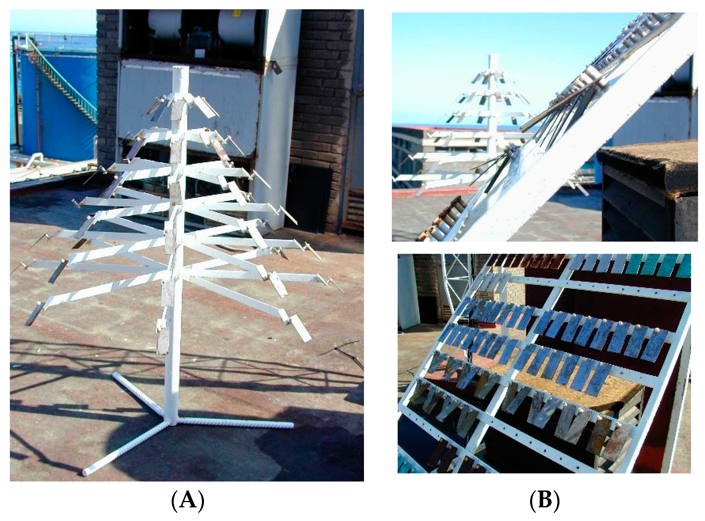
The test site consisted of two metallic frames on which the metal samples were attached using a nylon screw to avoid the formation of galvanic couples. For the orientation analysis, a tree-shaped metallic frame was built as shown in Figure 1A. The probes were located with an exposure angle of 45° and with eight different orientation angles (N, NE, E, SE, S, SW, W and NW). The distribution of the test panels in the different levels of this metallic frame prevented the downwards drainage of liquid or solid materials on the exposed panels. In a second metallic frame, carbon steel probes were placed with different exposure angles with respect to the horizontal (namely, 30°, 45° and 60°; see Figure 1B). The sensors for pollutants were located at the rear side of this frame, and they were collected on a monthly basis. The determination of sulphur dioxide pollution was made by the candle lead dioxide method according to the ASTM D 2010-85 norm [30]. Chloride measurements were performed using the wet candle method following the specifications of ISO 9225:1992 (E) [31].
The composition of the carbon steel samples is given in Table 2. Plates of approximate dimensions 100 mm × 40 mm × 20 mm were employed. The evaluation of the corrosion rates was made by weight loss of the samples according to the ASTM G1-90 norm [32]. Before being placed in the frames, the samples were marked for identification, cleaned according to the ASTM G1-90 norm [32], subsequently measured and weighed. Samples were collected from the test sites every two months for one year. Corrosion products were removed by chemical operation as described by the ASTM G1-90 standard [32]. After the samples were cleaned and dried, they were weighed again.
The time of wetness (TOW) was determined from the data collected using relative humidity hygrometers placed in a small cabinet at the rear of the station frames, and they were complemented with data supplied by the National Meteorological Institute of Spain (AEMET, Madrid, Spain). The latter were cumulative values taken over 8 h periods in a systematic way, whereas the autonomous hygrometers produced a continuous recording with autonomy for about one month. Data on the speed and direction of the winds were kindly supplied by AEMET.
3. Results and Discussion
3.1. Concentrations of Pollutants and Measurement of Corrosion Rates
The test site selected for this study was one of the used in the elaboration of the Corrosion Map of the Canary Islands where the carbon steel was one of the metals analysed [28]. In a recent review of the Corrosion Maps performed after the modification of the ISO 9223 norm [33], the previous results were confirmed [29]. Table 3 shows the amounts of pollutants as well as the TOW recorded bimonthly along the full period of study. The chloride levels obtained during the exposure time were constants with an average value of 74.98 ± 7.86 mg/(m2·day), whereas the sulphur dioxide (SO2) levels obtained show greater variability (5.14 ± 2.24 mg/(m2·day)). TOW increases linearly until 4312 h/year with a rate of increase 10 h/day. The main component of the winds is N-NE that corresponds with the Alisios Trade Winds affecting the Archipelago during most of the year.
3.2. Corrosion Rates
Table 4 shows the corrosion rates for the carbon steel samples exposed with different inclination and orientation angles. From an analysis of these data, it is observed that the corrosion rate varied with the exposure and orientation angles for each period of time under consideration. As for the exposure angle, the corrosion rates showed a maximum value of 71.39 μm/year and a minimum of 25.86 μm/year for all the periods. For one year of exposure, the higher corrosion rate corresponded to the carbon steel panels exposed with an angle of 30°, and the lowest corrosion rates for those exposed with 60°. For the sake of comparison, the 45° inclination as taken as reference because this is the typical exposure angle previously used all the studies of atmospheric corrosion that are carried in the North Hemisphere [6], and it was the exposure angles employed for the elaboration of the Corrosion Map of the Canary Islands [28,29].
In this way, it can be observed the corrosion rate was 29.1% greater for 30° and −5.6% for 60° exposure angles after 1-year exposure. The changes with the exposure angles determined for each time were not constant, and they showed a quasi-linear dependence. According to the data obtained in this work, the corrosion rate decreased with increasing exposure angles of the carbon steel panels, in good agreement with previous observations by other authors for carbon steel probes exposed to different atmospheres [10,12,34,35,36,37,38].
On the other hand, in regards to the corrosion rates determined for different orientation angles, a maximum corrosion rate of 64.24 μm/year and a minimum of 22.72 μm/year were obtained for all the periods. The corrosion rates for one year of exposure ranged between 22.70 (NW) and 24.65 (NE) μm/year (ca. 26.6% higher than those oriented to the south). The highest corrosion rates after one year of exposure were found for those steel panels oriented N-NE that were facing the prevailing winds. Figure 2 shows the evolution of the weight loss for each exposure angle (see Figure 2A) and orientation angle (Figure 2B). These results are in good agreement with those obtained for Vera et al. [10] in Chile in a similar test site.
In summary, according to the ISO 9223 norm [33], this test site shows a corrosivity category of C4, a S2 pollution level by airborne salinity (60 < Sd ≤ 300 mg/(m2·day)) and a P1 pollution level for by sulphur-containing substances represented by SO2 (4 < Pd ≤ 24 mg/(m2·day)), and a time of wetness (TOW) level of τ4 (2500 < τ ≤ 5500 h/year).
3.3. Mathematical Models
The mathematical models considered in this work were derived from the generic model showed in Equation (5), and they are listed next:
where CR is the corrosion rate expressed in μm/year; TEXP, the exposure time (year); TOW, time of wetness (year); CL, concentration of chlorides (g/(m2·year)); and SO2, concentration of SO2 (g/(m2·year)). The qualitative variables (O2 to O8) were included in Equations (7), (9), (11), (13) and (15) to produce changes in the independent coefficient k0 accounting for the different initial corrosion characteristics associated with the orientation of the probes. Analogously, I1 and I2 are qualitative variables included in Equations (7), (9), (11), (13) and (15) to produce changes in the independent coefficient k0 accounting for the different initial corrosion characteristics associated to the exposure angle of the probes.
The analysis of the different models was first performed considering the separate effects of the orientation and the exposure angle of the samples, and later evaluating their combined effect as they would operate together.
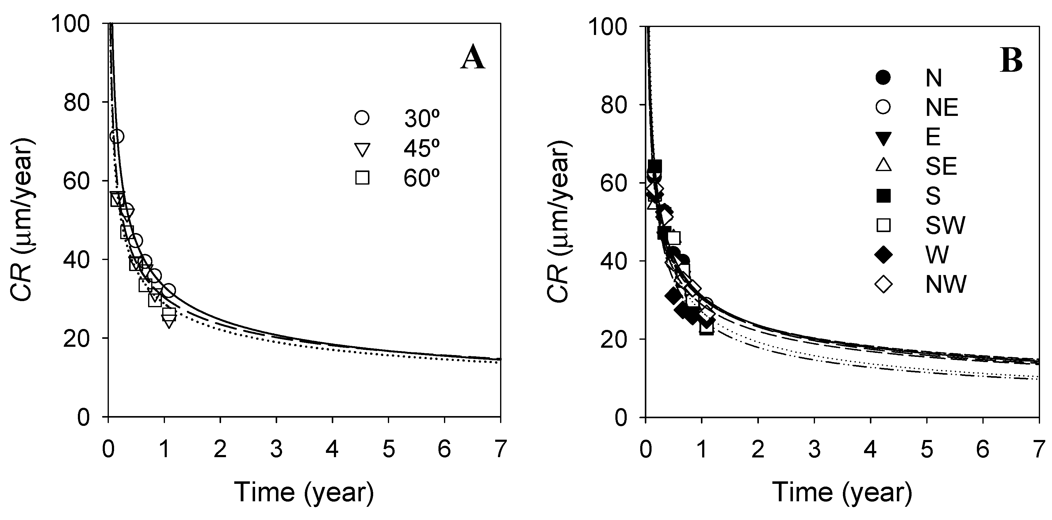
Figure 3 shows the corrosion rates measured for carbon steel panels exposed with different exposure and orientation angles as a function of elapsed time (cf. Figure 3A,B, respectively). It is observed that the data conformed to the potential law with a very good fit quality (R2 = 0.9999 for 30°, 0.8902 for 45°, and 0.9629 for 60° exposure angles), as shown in Table 5. When the evolution of the corrosion rate was analyzed exclusively in terms of the orientation angle, the bi-logarithmic model also fitted very well in most cases except for the SE orientation (namely, R2 = 0.7935; cf. Table 5). The results of the fists are given in the Supplementary Information, where Table S-1 shows the results using only the data related with the exposure angle, whereas Table S-2 shows those taking into account only the data according to the orientation angle.
3.3.1. Exposure Angle
When considering the models (6) and (8) taking TEXP as the only explanatory variable, it was found that both models exhibited similar fit qualities (= 0.8667 and 0.8974, respectively). In these models it was assumed that the exponent k1 depended on the variables corresponding to the environment [39], and they were further developed to account for the levels of chlorides, SO2 and TOW [40], producing the models (10), (12), (14) and (16). But the application of these new models did not produce any significant improvement as compared to the results obtained from the application of models (6) and (8).
From a more detailed analysis of the results, TOW was found to be the most significant variable among them. Since the different probes were exposed to the same levels of pollutants in the atmosphere, it was deduced that the lifetime of the water film over the surface of the probe must be an important factor influencing the corrosion rate. The actual levels of pollutants deposited on the metallic surface would depend on the exposure angle of the sample, and their effect should also depend on the kind of particle involved. On the other hand, the exposure angle can affect deposition of pollutants in two ways, namely gravitational settling of particles and condensation of water. According to Spence et al. [8], the deposition rate would be expected to be proportional to the projected horizontal area, which is given by the cosine of the exposure angle. Therefore, a bigger angle should facilitate the run-off of particles from the surface leading to a decrease in the corrosion rate of the metal. The new models described by Equations (7), (9), (11), (13), (15) and (17) were obtained by introducing a new qualitative variable related to the exposure angle, I. These models showed better fit qualities than the corresponding ones without the qualitative variable, although major differences between them was not observed (≈ 0.98 for all of them) except for model (7) (with = 0.9482). The estimation of the parameter of the qualitative variable related to the inclination angle of 30°, I1, indicates a greater effect than for 45°, with an increase of 9.41%. The estimation of the parameter related to I2 shows a negative value in relation to the reference angle, with a fall of 8.24%. This is in good agreement with the corrosion rates observed so to biggest angles lowest corrosion rates.
3.3.2. Orientation Angle
The data were fitted with the models (6)–(17) where the orientation angle is introduced as explanatory variable (O) together with the levels of pollutants, TOW and TEXP. In this case, the inclination angle was fixed at 45° because it is the typical procedure employed for this geographical zone.
From an analysis of the models (6) to (9), models (6) and (7) exhibited better fit qualities (i.e., = 0.9194 and 0.9363, respectively) than models (8) and (9). In the latter, although model (9) includes the qualitative variable O, the obtained fit did not improve compared to that with model (8). In models (10) to (17), the variables related with the levels of pollutants and the TOW are included, being the models with the qualitative variables those delivering the best fits. Indeed, the best regression indexes (namely, = 0.9401) were obtained for the models (15) and (17). In this case, all the coefficients related with the qualitative variables were negative. This feature implies that lower corrosion rates will be obtained with regards to the panels oriented to the North, with the biggest reductions occurring for the orientations East (O3), South (O5) and West (O7), with ratios of 7.91%, 7.47% and 14.91%, respectively.
3.3.3. Global Mode
In the previous two sections, the fits were obtained by working solely on either the exposure or the orientation angles. With the aim of obtaining a global model including all the variables, models (6)–(17) were next applied to the whole set of data. The results are shown in Table 6. It can be concluded that the models including the qualitative variables showed very good fit qualities, being difficult to make a clear distinction among them based on their performance (that is, > 0.91 in all the cases). Anyway, those models including the environmental variables (i.e., models (11), (13), (15) and (17)) exhibited the best fits (with > 0.94) in comparison with models (7) and (9).
It can be concluded that the models including the qualitative variables showed very good fit qualities, being difficult to make a clear distinction among them based on their performance (that is, > 0.91 in all the cases). Anyway, those models including the environmental variables (i.e., models (11), (13), (15) and (17)) exhibited the best fits (with > 0.94) in comparison with models (7) and (9).
From the foregoing, it can be concluded that model (18) would be a good mathematical model to describe all the effects participating in an atmospheric corrosion process as it accounts for the effect of the pollutants, TOW, time of exposure, as well as the exposure angle and the orientation of the test panels.
4. Conclusions
The corrosive process occurring on carbon steel specimens exposed in a marine test site has been characterized taking into account the exposure angle and the orientation of the probes. It was found that the corrosion rates would diminish with greater exposure angles, in good accordance with previous reports in the literature. Next, the carbon steel probes with N-NE orientation were those with the highest corrosion rates because they were directly facing the prevailing winds.
Although data could be adjusted to the bi-logarithmic law with good fits when either the exposure angle or the orientation were considered separately, the fits became worst when all the data were taken into account simultaneously. The quality of the fits could be improved with respect to the bi-logarithmic law models when the variable concentration of pollutants and TOW were introduced in the model, but not to full satisfaction. A definite improvement of the model was attained by incorporating qualitative variables, thus leading to obtaining a global model with a high degree of adjustment (= 0.99), being the first mathematical model to incorporate the effect of inclination and orientation together.
Supplementary Materials
The following are available online at https://www.mdpi.com/2075-4701/10/2/196/s1, Table S-1: Values of the constants ki and δi in the models (6) to (15) when considering solely the effect of the exposure angle (i.e., δi = 0 in all cases); and Table S-2: Values of the constants ki and δi in the models (6) to (15) when considering solely the effect of the orientation (i.e., γn = 0 in all cases).
Author Contributions
Conceptualization, J.J.S and R.M.S.; methodology, J.J.S., R.M.S. and H.C.V.; software, J.J.S. and V.C.; validation, J.J.S., V.C., R.M.S. and H.C.V.; formal analysis, J.J.S., R.M.S. and V.C.; investigation, J.J.S., V.C., H.C.V. and R.M.S.; resources, J.J.S. and R.M.S.; data curation, J.J.S. and V.C.; writing—original draft preparation, J.J.S. and H.C.V.; writing—review and editing, J.J.S. and R.M.S.; visualization, J.J.S. and R.M.S.; supervision, J.J.S. and R.M.S.; project administration, J.J.S. and R.M.S.; funding acquisition, J.J.S. and R.M.S. All authors have read and agreed to the published version of the manuscript.
Funding
This research was funded by the Canarian Agency for Research, Innovation and Information Society (Las Palmas de Gran Canaria, Spain) and the European Social Fund (Brussels, Belgium) under grant ProID2017010042.
Conflicts of Interest
The authors declare no conflict of interest.
References
- Ghali, E.; Sastri, V.S.; Elboujdaini, M. Corrosion Prevention and Protection. Practical Solutions; John Wiley & Sons, Ltd.: Chichester, UK, 2007; ISBN 9780470024546. [Google Scholar]
- Cramer, S.D.; Covino, B.S., Jr. Corrosion, Fundamentals, Testing and Applications, ASM Handbook Series, 1st ed.; American Society for Testing Materials Int.: Columbus, OH, USA, 2003; Volume 13A, ISBN 978-1-62708-182-5. [Google Scholar]
- Schweitzer, P.A. Fundamentals of Metallic Corrosion; CRC Press: Boca Raton, FL, USA, 2006; ISBN 9780429127137. [Google Scholar]
- Leygraf, C.; Wallinder, I.O.; Tidblad, J.; Graedel, T. Atmospheric Corrosion; John Wiley & Sons, Inc.: Hoboken, NJ, USA, 2016; ISBN 9781118762134. [Google Scholar]
- Schweitzer, P.A. Atmospheric Degradation and Corrosion Control; CRC Press: New York, NY, USA, 1999; ISBN 9780824777098. [Google Scholar]
- Veleva, L.; Kane, R.D. Atmospheric corrosion. In ASM Handbook Volume 13A: Corrosion: Fundamentals, Testing, and Protection; Cramer, S.D., Covino, B.S., Jr., Eds.; American Society for Testing Materials Int.: Columbus, OH, USA, 2003; Volume 13A, pp. 196–209. ISBN 978-0-87170-705-5. [Google Scholar]
- Giardina, M.; Buffa, P. A new approach for modeling dry deposition velocity of particles. Atmos. Environ. 2018, 180, 11–22. [Google Scholar] [CrossRef]
- Spence, J.W.; Lipfert, F.W.; Katz, S. The effect of specimen size, shape, and orientation on dry deposition to galvanized steel surfaces. Atmos. Environ. Part A. Gen. Top. 1993, 27, 2327–2336. [Google Scholar] [CrossRef]
- Morcillo, M.; Chico, B.; Díaz, I.; Cano, H.; de la Fuente, D. Atmospheric corrosion data of weathering steels. A review. Corros. Sci. 2013, 77, 6–24. [Google Scholar] [CrossRef] [Green Version]
- Vera, R.; Rosales, B.M.; Tapia, C. Effect of the exposure angle in the corrosion rate of plain carbon steel in a marine atmosphere. Corros. Sci. 2003, 45, 321–337. [Google Scholar] [CrossRef]
- Edney, E.O.; Cheek, S.F.; Stiles, D.C.; Corse, E.W. Field study investigations of the impact of shape, size and orientation on dry deposition induced corrosion of galvanized steel. Atmos. Environ. Part A. Gen. Top. 1992, 26, 2353–2363. [Google Scholar] [CrossRef]
- Coburn, S.K.; Komp, M.E.; Lore, S.C. Atmospheric corrosion rates of weathering steels at test sites in the Eastern United States—Effect of environment and test-panel orientation. In Atmospheric Corrosion; Kirk, W., Lawson, H., Eds.; ASTM STP 1239; American Society for Testing Materials Int.: West Conshocken, PA, USA, 1995; pp. 100–113. [Google Scholar]
- Vasconcelos, H.C.; Fernández-Pérez, B.M.; Morales, J.; Souto, R.M.; González, S.; Cano, V.; Santana, J.J. Development of mathematical models to predict the atmospheric corrosion rate of carbon steel in fragmented subtropical environments. Int. J. Electrochem. Sci. 2014, 9, 6514–6528. [Google Scholar]
- Spence, J.W.; McHenry, J.N. Development of regional corrosion maps for galvanized steel by linking the RADM engineering model with an atmospheric corrosion model. Atmos. Environ. 1994, 28, 3033–3046. [Google Scholar] [CrossRef]
- Feliu, S.; Morcillo, M.; Feliu, S. The prediction of atmospheric corrosion from meteorological and pollution parameters—II. Long-term forecasts. Corros. Sci. 1993, 34, 415–422. [Google Scholar] [CrossRef]
- Tidblad, J.; Mikhailov, A.; Kucera, V. Application of a model for prediction of atmospheric corrosion in tropical environments. In Marine Corrosion in Tropical Environments; Dean, S., Delgadillo, G.-D., Bushman, J., Eds.; ASTM International: West Conshohocken, PA, USA, 2000; pp. 250–285. ISBN 978-0-8031-2873-6. [Google Scholar]
- Tidblad, J.; Kucera, V.; Mikhailov, A.; Knotkova, D. Improvement of the ISO classification system based on dose-response functions describing the corrosivity of outdoor atmospheres. In Outdoor Atmospheric Corrosion; Townsend, H.E., Ed.; ASTM International: West Conshohocken, PA, USA, 2002; pp. 73–87. ISBN 978-0-8031-5467-4. [Google Scholar]
- Spence, J.W.; Haynie, F.H.; Lipfert, F.W.; Cramer, S.D.; McDonald, L.G. Atmospheric corrosion model for galvanized steel structures. Corrosion 1992, 48, 1009–1019. [Google Scholar] [CrossRef]
- Pourbaix, M. The linear bilogarithmic law for atmospheric corrosion. In Atmospheric Corrosion; Ailor, W.H., Ed.; J. Wiley & Sons: New York, NY, USA, 1982; pp. 107–121. [Google Scholar]
- Panchenko, Y.M.; Strekalov, P.V. Correlation between corrosion mass losses and corrosion product quantity retained on metals in a cold, moderate and tropical climate. Prot. Met. 1994, 30, 459–467. [Google Scholar]
- Morcillo, M.; Feliu, S.; Simancas, J. Deviation from bilogarithmic law for atmospheric corrosion of steel. Br. Corros. J. 1993, 28, 50–52. [Google Scholar] [CrossRef] [Green Version]
- Almeida, E.; Morcillo, M.; Rosales, B.; Marrocos, M. Atmospheric corrosion of mild steel. Part I—Rural and urban atmospheres. Mater. Corros. 2000, 51, 859–864. [Google Scholar] [CrossRef]
- Almeida, E.; Morcillo, M.; Rosales, B. Atmospheric corrosion of mild steel. Part II—Marine atmospheres. Mater. Corros. 2000, 51, 865–874. [Google Scholar] [CrossRef]
- Graedel, T.E. Corrosion mechanisms for iron and low alloy steels exposed to the atmosphere. J. Electrochem. Soc. 1990, 137, 2385. [Google Scholar] [CrossRef]
- Kamimura, T.; Hara, S.; Miyuki, H.; Yamashita, M.; Uchida, H. Composition and protective ability of rust layer formed on weathering steel exposed to various environments. Corros. Sci. 2006, 48, 2799–2812. [Google Scholar] [CrossRef]
- Santana Rodríguez, J.J.; Santana Hernández, F.J.; González González, J.E. Mathematical and electro-chemical characterisation of the layer of corrosion products on carbon steel in various environments. Corros. Sci. 2002, 44, 2597–2610. [Google Scholar] [CrossRef]
- Zoccola, J.C.; Permoda, A.J.; Oehler, L.T.; Horton, J.B. Performance of Mayari R Weathering Steel (ASTM A242) in Bridges at the Eight Mile Road and John Lodge Expressway in Detroit, Michigan. Bethlehem Steel Corporation: Bethlehem, PA, USA. Available online: https://www.michigan.gov/documents/mdot/RR213CON_67_534507_7.pdf (accessed on 28 January 2020).
- Santana, J.J.; Santana, F.J.; González, J.E.; de la Fuente, D.; Chico, B.; Morcillo, M. Atmospheric corrosivity map for steel in Canary Isles. Br. Corros. J. 2001, 36, 266–271. [Google Scholar] [CrossRef] [Green Version]
- Santana, J.J.; Ramos, A.; Rodriguez-Gonzalez, A.; Vasconcelos, H.C.; Mena, V.; Fernández-Pérez, B.M.; Souto, R.M. Shortcomings of International Standard ISO 9223 for the classification, determination, and estimation of atmosphere corrosivities in subtropical archipelagic conditions—The case of the Canary Islands (Spain). Metals 2019, 9, 1105. [Google Scholar] [CrossRef] [Green Version]
- ASTM D2010/D2010M-98(2017), Standard Test Methods for Evaluation of Total Sulfation Activity in the Atmosphere by the Lead Dioxide Technique; ASTM International: West Conshohocken, PA, USA, 2017.
- ISO 9225:2012, Corrosion of Metals and Alloys—Corrosivity of Atmospheres—Measurement of Environmental Parameters Affecting Corrosivity of Atmospheres, 2nd ed.; International Organization for Standardization: Geneva, The Switzerland, 2012.
- ASTM G1-90, Standard Practice for Preparing, Cleaning, and Evaluating Corrosion Test Specimens; American Society for Testing Materials: Philadelphia, PA, USA, 1990.
- ISO 9223:2012, Corrosion of Metals and Alloys—Corrosivity of Atmospheres—Clasification, Determination and Estimation, 2nd ed.; International Organization for Standardization: Geneva, The Switzerland, 2012.
- Larrabee, C.P. Corrosion resistance of high-strength low-alloy steels as influenced by composition and environment. Corrosion 1953, 9, 259–271. [Google Scholar] [CrossRef]
- LaQue, F.L. Corrosion testing. In ASTM Proceeding 1951—Volume 51; American Society for Testing and Materials: Philadelphia, PA, USA, 1951; Volume 51, pp. 495–582. [Google Scholar]
- Binh, D.T.; Strekalov, P.V.; Van Khuong, N. Effects of seasonal conditions and the slope of a specimen on the atmospheric corrosion of steel in the tropics of Viet-Nam. Prot. Met. 2003, 39, 278–287. [Google Scholar] [CrossRef]
- Veleva, L.; Maldonado, L. Classification of atmospheric corrosivity in humid tropical climates. Br. Corros. J. 1998, 33, 53–58. [Google Scholar] [CrossRef]
- Rostron, P.; Belbarak, C. Atmospheric corrosion issues in Abu Dhabi. Mater. Perform. 2015, 54, 1–7. [Google Scholar]
- Porro, A.; Otero, T.F.; Elola, A.S. Gravimetric corrosion monitoring and mathematical fitting of atmospheric corrosion data for carbon steel. Br. Corros. J. 1992, 27, 231–235. [Google Scholar] [CrossRef]
- Santana Rodríguez, J.J.; Santana Hernández, F.J.; González González, J.E. XRD and SEM studies of the layer of corrosion products for carbon steel in various different environments in the province of Las Palmas (The Canary Islands, Spain). Corros. Sci. 2002, 44, 2425–2438. [Google Scholar] [CrossRef]
Figure 1.
Metallic frames employed to expose the carbon steel panels for the investigation of the influence of (A) the orientation and (B) the exposure angles on the atmospheric corrosion rate.
Figure 1.
Metallic frames employed to expose the carbon steel panels for the investigation of the influence of (A) the orientation and (B) the exposure angles on the atmospheric corrosion rate.

Figure 2.
Weight loss of carbon steel as a function of time for panels exposed with varying: (A) exposure angles with respect to the horizontal, and (B) orientations.
Figure 2.
Weight loss of carbon steel as a function of time for panels exposed with varying: (A) exposure angles with respect to the horizontal, and (B) orientations.
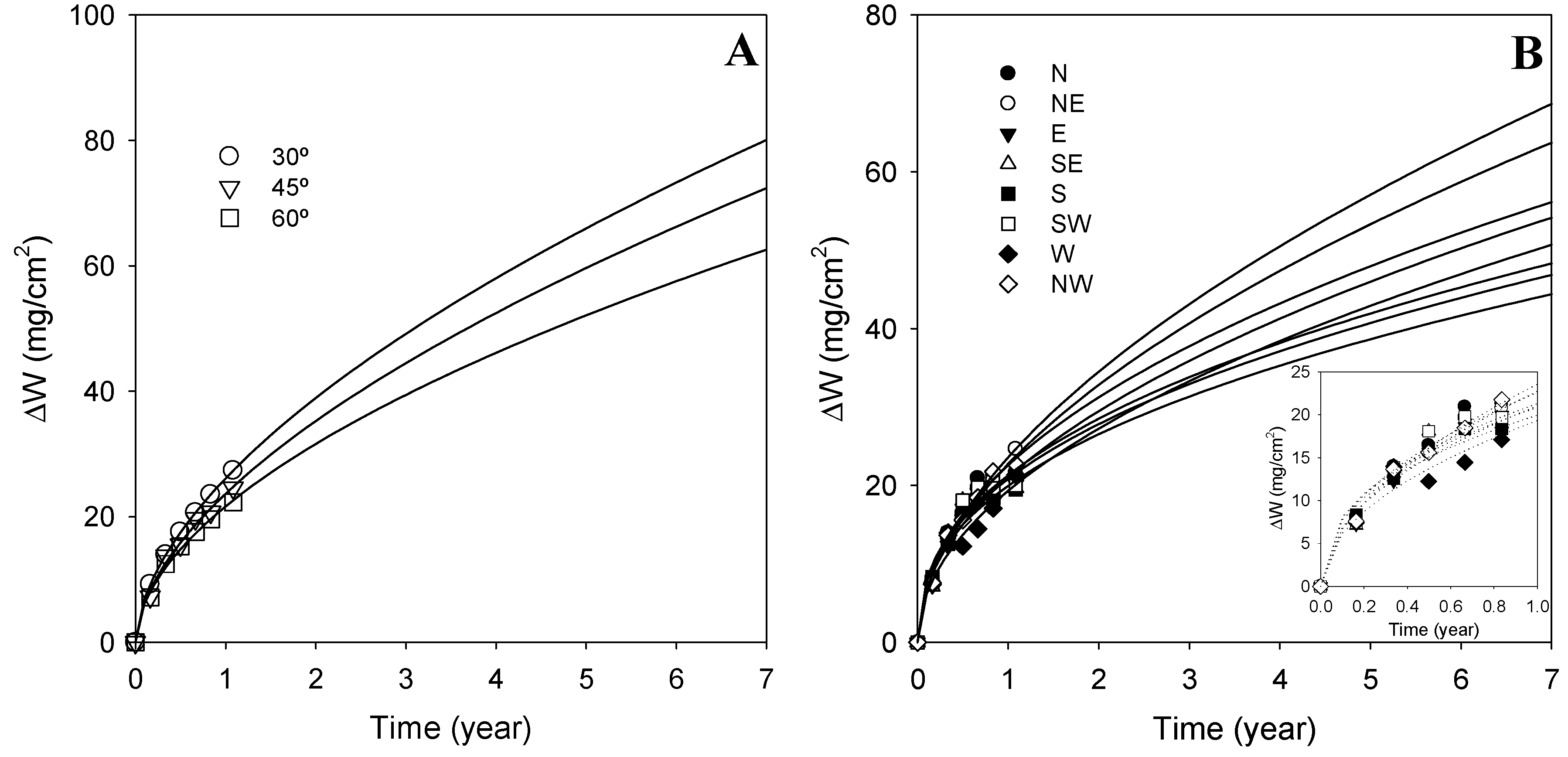
Figure 3.
Data fitting to the bi-logarithmic law for the corrosion rates of carbon steel panels exposed with varying: (A) exposure angles with respect to the horizontal, and (B) orientations.
Figure 3.
Data fitting to the bi-logarithmic law for the corrosion rates of carbon steel panels exposed with varying: (A) exposure angles with respect to the horizontal, and (B) orientations.


Table 1.
Location and characteristic environment type of the test site.
| Test Site | Elevation (m) | Geographic Coordinate | Atmosphere | |
|---|---|---|---|---|
| North Latitude | West Longitude | |||
| Power station of Jinámar | 30 | 28° 02′ 30″ N | 15° 24′ 39″ W | Industrial marine |
Table 2.
Composition of the carbon steel.
| Composition (wt. %) | ||||||||||
|---|---|---|---|---|---|---|---|---|---|---|
| Si | Fe | C | Mn | Zn | Ti | Cu | Mg | Al | Others | Fe |
| 0.08 | 99.47 | 0.06 | 0.37 | - | - | - | - | - | 0.02 | balance |
Table 3.
Chloride and sulphur dioxide deposition rates and time of wetness recorded bimonthly at the test station over one year.
Table 3.
Chloride and sulphur dioxide deposition rates and time of wetness recorded bimonthly at the test station over one year.
| Exposure Time (day) | SO2 (mg/(m2·day)) | Cl− (mg/(m2·day)) | TOW (h/year) |
|---|---|---|---|
| 60 | 2.99 | 85.43 | 862 |
| 123 | 2.17 | 78.10 | 1552 |
| 182 | 4.47 | 80.86 | 1897 |
| 243 | 6.74 | 68.45 | 2673 |
| 305 | 7.12 | 64.68 | 3553 |
| 396 | 7.33 | 72.36 | 4312 |
Table 4.
Variation of the corrosion rates measured with different exposure angles and orientations of the carbon steel panels. N (north), NE (northeast), E (east), SE (southeast), S (south), SW (southwest), W (west), NW (northwest).
Table 4.
Variation of the corrosion rates measured with different exposure angles and orientations of the carbon steel panels. N (north), NE (northeast), E (east), SE (southeast), S (south), SW (southwest), W (west), NW (northwest).
| Time (day) | rcorr (µm/year) | ||||||||||
|---|---|---|---|---|---|---|---|---|---|---|---|
| Exposure Angle | Orientation | ||||||||||
| 30° | 45° | 60° | N | NE | E | SE | S | SW | W | NW | |
| 60 | 71.1 | 56.1 | 55.1 | 61.38 | 62.60 | 56.15 | 54.40 | 64.22 | 56.91 | 57.07 | 58.53 |
| 123 | 52.4 | 51.7 | 46.9 | 52.52 | 51.72 | 46.29 | 51.82 | 47.19 | 52.03 | 52.50 | 51.26 |
| 182 | 44.6 | 39.5 | 38.8 | 41.77 | 39.46 | 39.70 | 45.86 | 40.88 | 45.86 | 31.08 | 39.60 |
| 243 | 39.3 | 37.5 | 33.4 | 39.78 | 37.51 | 36.22 | 36.91 | 34.87 | 37.57 | 27.48 | 35.10 |
| 305 | 35.7 | 31.4 | 29.6 | 32.25 | 31.44 | 30.19 | 28.63 | 27.81 | 29.78 | 25.89 | 32.96 |
| 396 | 31.9 | 24.7 | 26.0 | 25.18 | 28.76 | 23.50 | 22.92 | 22.72 | 23.33 | 24.91 | 26.48 |
Table 5.
Values of the k and n constants for the potential law model (CR in µm/year) and fit quality.
Table 5.
Values of the k and n constants for the potential law model (CR in µm/year) and fit quality.
| Constants | Exposure Angle | Orientation | |||||||||
|---|---|---|---|---|---|---|---|---|---|---|---|
| 30° | 45° | 60° | N | NE | E | SE | S | SW | W | NW | |
| k | 33.0920 (0.049) | 30.3580 (2.3768) | 28.7564 (1.2736) | 31.1281 (2.1182) | 30.6990 (1.3036) | 28.8354 (1.6732) | 30.4171 (3.4883) | 27.0422 (1.3639) | 30.7166 (3.1321) | 25.0282 (3.0355) | 30.3778 (1.7038) |
| n | −0.4236 (0.0012) | −0.3714 (0.06505) | −0.3789 (0.03663) | −0.3993 (0.0556) | −0.4079 (0.0345) | −0.3877 (0.04774) | −0.3687 (0.0954) | −0.4901 (0.0392) | −0.3810 (0.0842) | −0.4847 (0.0944) | −0.3848 (0.0462) |
| 0.9999 | 0.8902 | 0.9629 | 0.9273 | 0.9710 | 0.9419 | 0.7935 | 0.9795 | 0.8392 | 0.8664 | 0.9441 | |
Notes: Standard errors are given within brackets below the corresponding estimated coefficient.
Table 6.
Values of the constants ki, δi and γi obtained from the application of models (6)–(15).
| Variables | Model (6) | Model (7) | Model (8) | Model (9) | Model (10) | Model (11) | Model (12) | Model (13) | Model (14) | Model (15) | Model (16) | Model (17) |
|---|---|---|---|---|---|---|---|---|---|---|---|---|
| Constant | 4.2192 * (0.0258) | 4.2484 * (0.0353) | 3.3580 * (0.0190) | 3.3943 * (0.0379) | 4.2499 * (0.2587) | 4.2862 * (0.1851) | 3.8302 * (0.2637) | 3.8666 * (0.1887) | 5.2157 * (0.7226) | 5.2521 * (0.5119) | 4.7733 * (0.6890) | 4.8097 * (0.4880) |
| TEXP | −0.9193 * (0.0385) | −0.9193 * (0.0289) | - | - | - | - | - | - | - | - | - | - |
| SO2 | - | - | - | - | −0.0726 ** (0.0383) | −0.0726 * (0.0271) | −0.1092 * (0.0345) | −0.1092 * (0.0245) | - | - | - | - |
| CL | - | - | - | - | −0.0133 (0.0082) | −0.0133 ** (0.0058) | −0.0287 * (0.0093) | −0.0287 * (0.0066) | - | - | - | - |
| TOW | - | - | - | - | −0.8768 * (0.2996) | −0.8768 * (0.2121) | - | - | - | - | −0.9763 * (0.2796) | −0.9763 * (0.1978) |
| LTEXP | - | - | −0.4463 * (0.0206) | −0.4463 * (0.0167) | −0.2363 * (0.0616) | −0.2363 * (0.0435) | 0.1289 (0.1760) | 0.1289 (0.1247) | 0.2260 (0.1800) | 0.2260 *** (0.1274) | −0.2211 * (0.0612) | −0.2211 * (0.0395) |
| LSO2 | - | - | - | - | - | - | - | - | −0.1547 * (0.0486) | −0.1547 * (0.0332) | −0.0963 *** (0.0489) | −0.0963 * (0.0346) |
| LCL | - | - | - | - | - | - | - | - | −0.7264 * (0.2455) | −0.7264 * (0.01737) | −0.2828 (0.2066) | −0.2828 *** (0.1461) |
| LTOW | - | - | - | - | - | - | −0.6523 * (0.2236) | −0.6523 * (0.1584) | −0.7762 * (0.2225) | −0.7762 * (0.1574) | - | - |
| O2 | - | −0.0006 (0.0434) | - | −0.0006 (0.0511) | - | −0.0006 (0.0396) | - | −0.0006 (0.0396) | - | −0.0006 (0.0439) | - | −0.0006 (0.0395) |
| O3 | - | −0.0825 ** (0.0434) | - | −0.0824 (0.0511) | - | −0.0824 ** (0.0396) | - | −0.0824 ** (0.0396) | - | −0.0824 ** (0.0439) | - | −0.0824 ** (0.0395) |
| O4 | - | −0.0548 (0.0434) | - | −0.0548 (0.0511) | - | −0.0548 (0.0396) | - | −0.0548 (0.0396) | - | −0.0548 (0.0441) | - | −0.0548 (0.0395) |
| O5 | - | −0.0777 *** (0.0434) | - | −0.0776 (0.0511) | - | −0.0776 *** (0.0396) | - | −0.0776 *** (0.0396) | - | −0.0776 *** (0.0439) | - | −0.0776 *** (0.0395) |
| O6 | - | −0.0341 (0.0434) | - | −0.0341 (0.0511) | - | −0.0341 (0.0396) | - | −0.0341 (0.0396) | - | −0.0341 (0.0439) | - | −0.0341 (0.0395) |
| O7 | - | −0.1615 * (0.0434) | - | −0.1615 * (0.0511) | - | −0.1615 * (0.0396) | - | −0.1615 * (0.0396) | - | −0.1615 * (0.0439) | - | −0.1615 * (0.0395) |
| O8 | - | −0.0297 (0.0434) | - | −0.0297 (0.0511) | - | −0.0297 (0.0396) | - | −0.0297 (0.0396) | - | −0.0297 (0.0439) | - | −0.0297 (0.0395) |
| I1 | - | 0.0899 * (0.0377) | - | 0.0899 * (0.0443) | - | 0.0899 ** (0.0343) | - | 0.0899 ** (0.0343) | - | 0.0899 ** (0.0343) | - | 0.0899 ** (0.0342) |
| I2 | - | −0.0864 ** (0.0377) | - | −0.0864 * (0.0443) | - | −0.0864 ** (0.0343) | - | −0.0864 ** (0.0343) | - | −0.0864 ** (0.0343) | - | −0.0864 ** (0.0342) |
| 0.8908 | 0.9373 | 0.8684 | 0.9133 | 0.8964 | 0.9480 | 0.8964 | 0.9480 | 0.8966 | 0.9482 | 0.8966 | 0.9483 | |
| N | 72 | 72 | 72 | 72 | 72 | 72 | 72 | 72 | 72 | 72 | 72 | 72 |
Notes: Standard errors are given within brackets below the corresponding estimated coefficient; * Significant at 1% level. ** Significant at 5% level. *** Significant at 10% level.
© 2020 by the authors. Licensee MDPI, Basel, Switzerland. This article is an open access article distributed under the terms and conditions of the Creative Commons Attribution (CC BY) license (http://creativecommons.org/licenses/by/4.0/).
Share and Cite
MDPI and ACS Style
Santana, J.J.; Cano, V.; Vasconcelos, H.C.; Souto, R.M. The Influence of Test-Panel Orientation and Exposure Angle on the Corrosion Rate of Carbon Steel. Mathematical Modelling. Metals 2020, 10, 196. https://doi.org/10.3390/met10020196
AMA Style
Santana JJ, Cano V, Vasconcelos HC, Souto RM. The Influence of Test-Panel Orientation and Exposure Angle on the Corrosion Rate of Carbon Steel. Mathematical Modelling. Metals. 2020; 10(2):196. https://doi.org/10.3390/met10020196
Chicago/Turabian StyleSantana, Juan J., Víctor Cano, Helena C. Vasconcelos, and Ricardo M. Souto. 2020. "The Influence of Test-Panel Orientation and Exposure Angle on the Corrosion Rate of Carbon Steel. Mathematical Modelling" Metals 10, no. 2: 196. https://doi.org/10.3390/met10020196
Note that from the first issue of 2016, this journal uses article numbers instead of page numbers. See further details here.