Liquid Metal Flow Under Traveling Magnetic Field—Solidification Simulation and Pulsating Flow Analysis


Abstract
1. Introduction
2. Methods
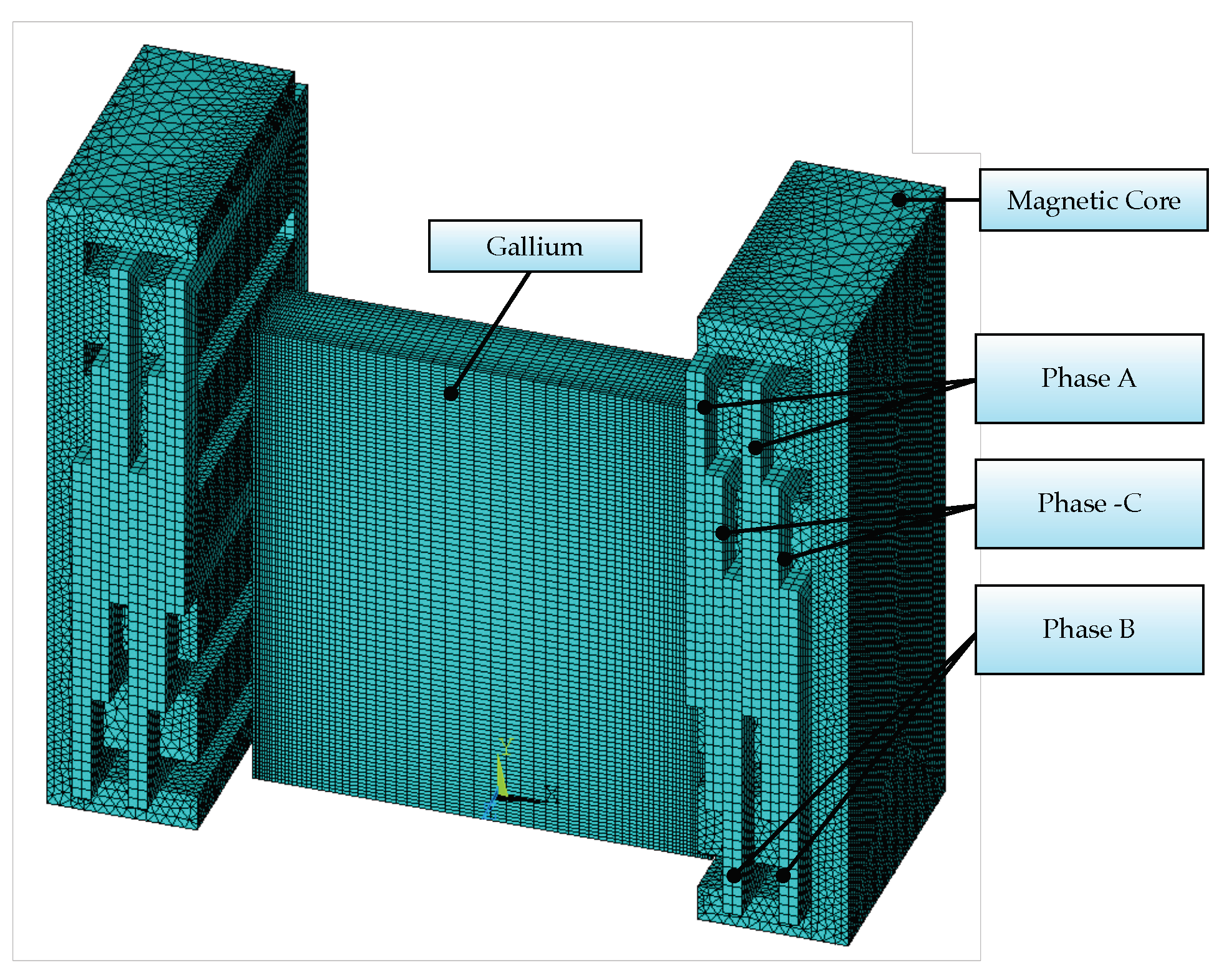
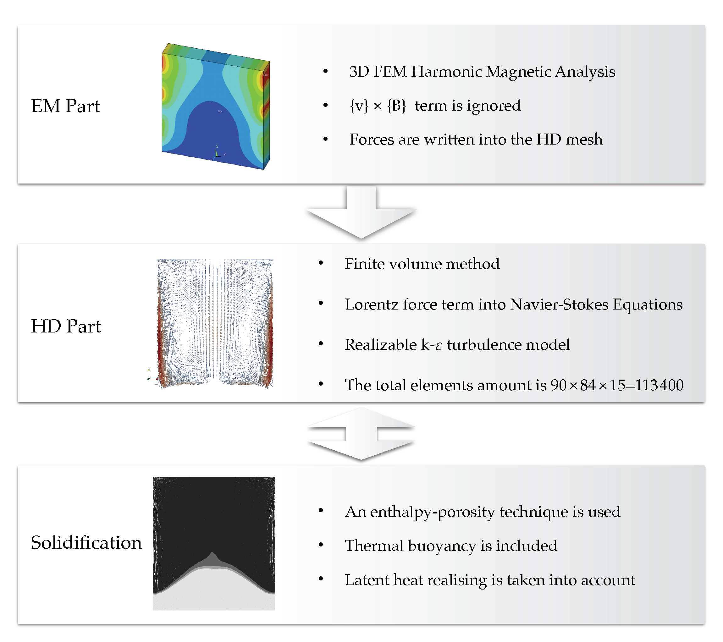
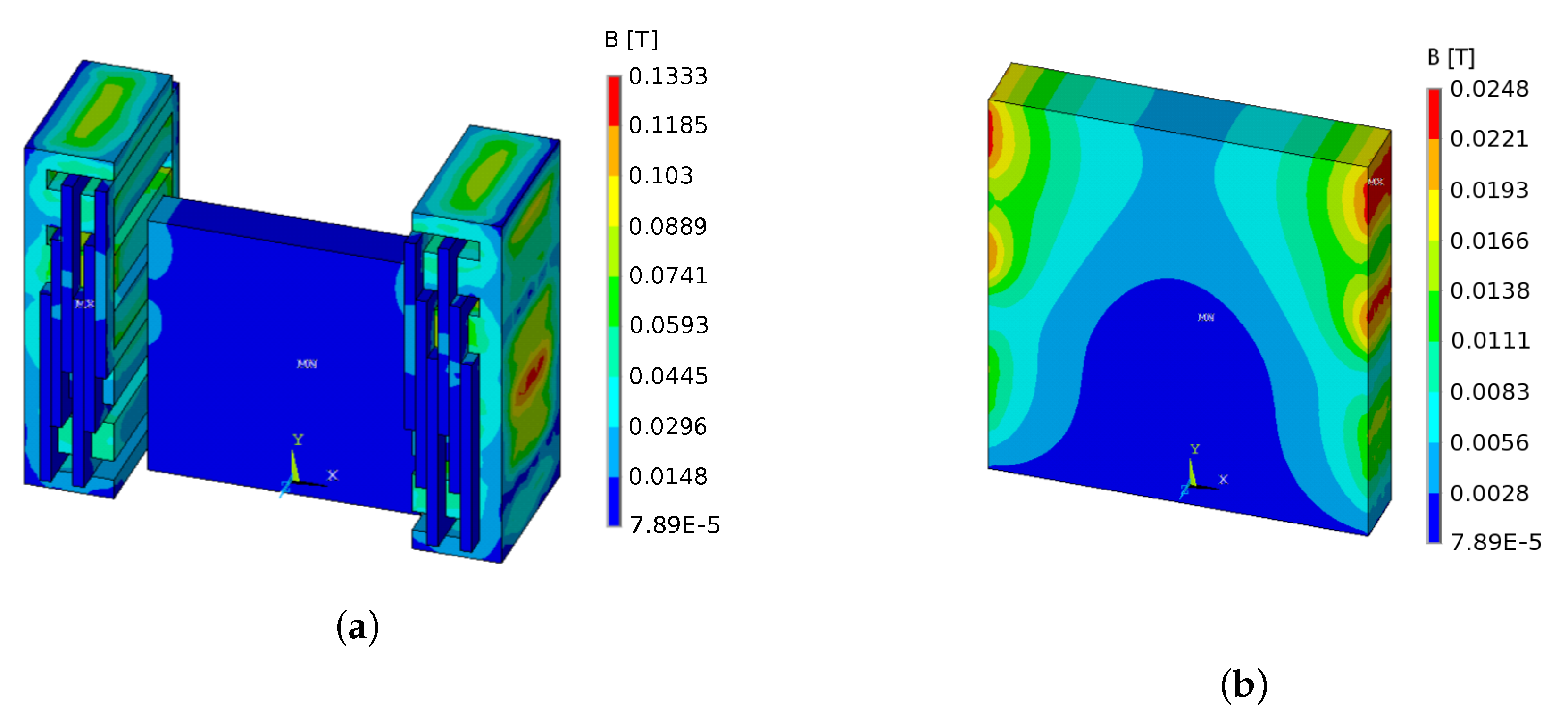
2.1. Electromagnetic Part
2.1.1. Governing Equations
2.1.2. Boundary Conditions and Numerical Mesh
2.2. Hydrodynamic Part
2.2.1. RANS Modeling
2.2.2. LES Approach
2.3. Solidification
2.4. Simulation Coupling
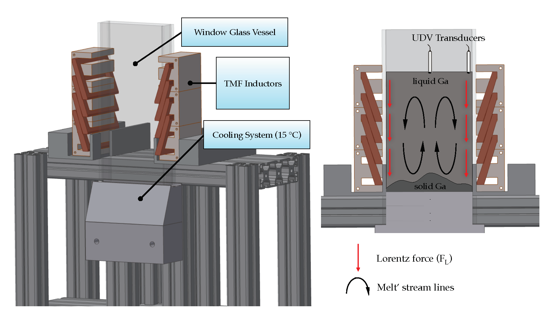
2.4.1. Experimental Setup and Validation
2.4.2. UDV Measurements
2.4.3. Neutron Radiography Visualisation
3. Results
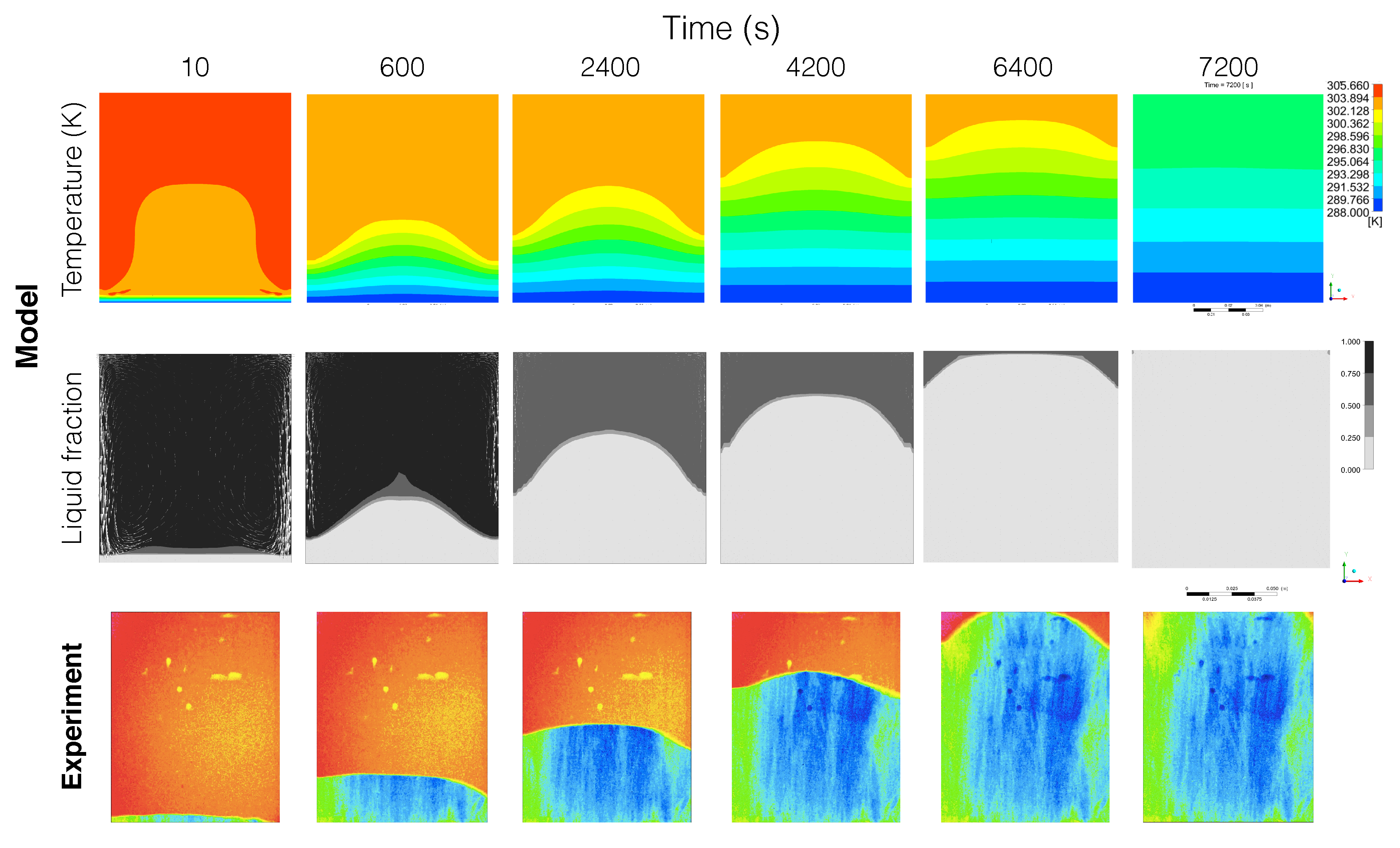
3.1. Solidification
3.2. Pulsed TMF Study
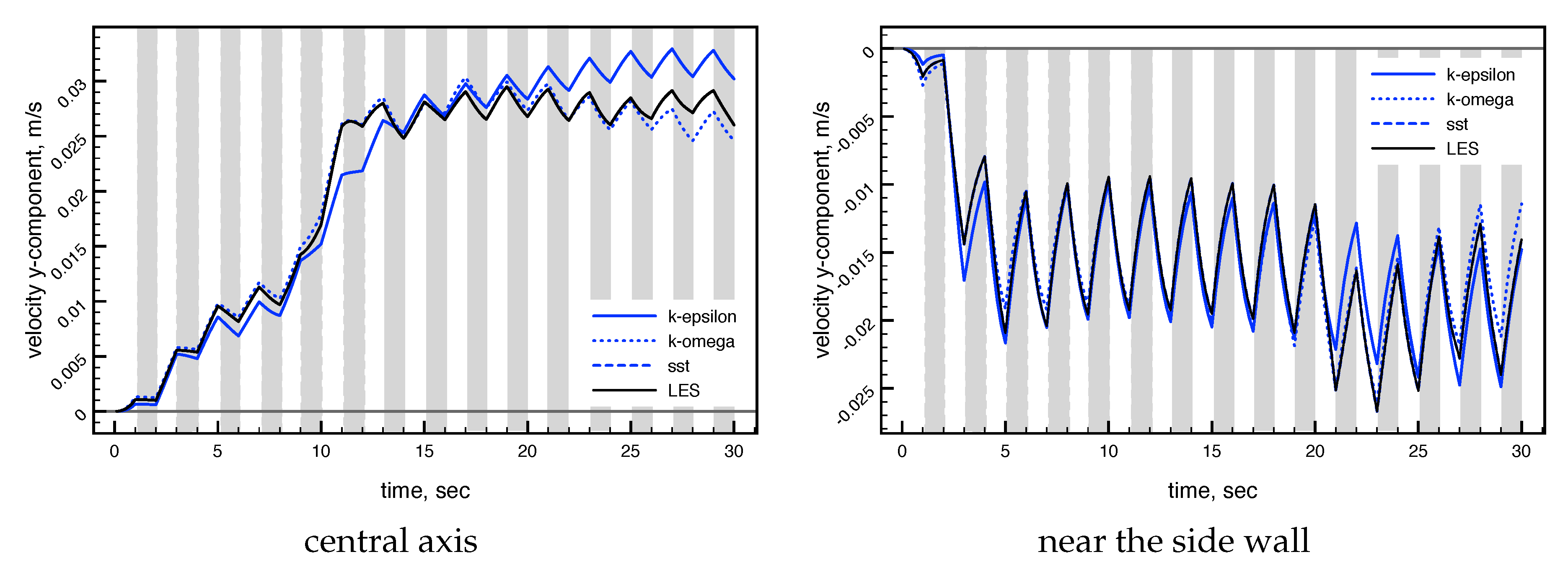
3.2.1. Turbulence Model Testing
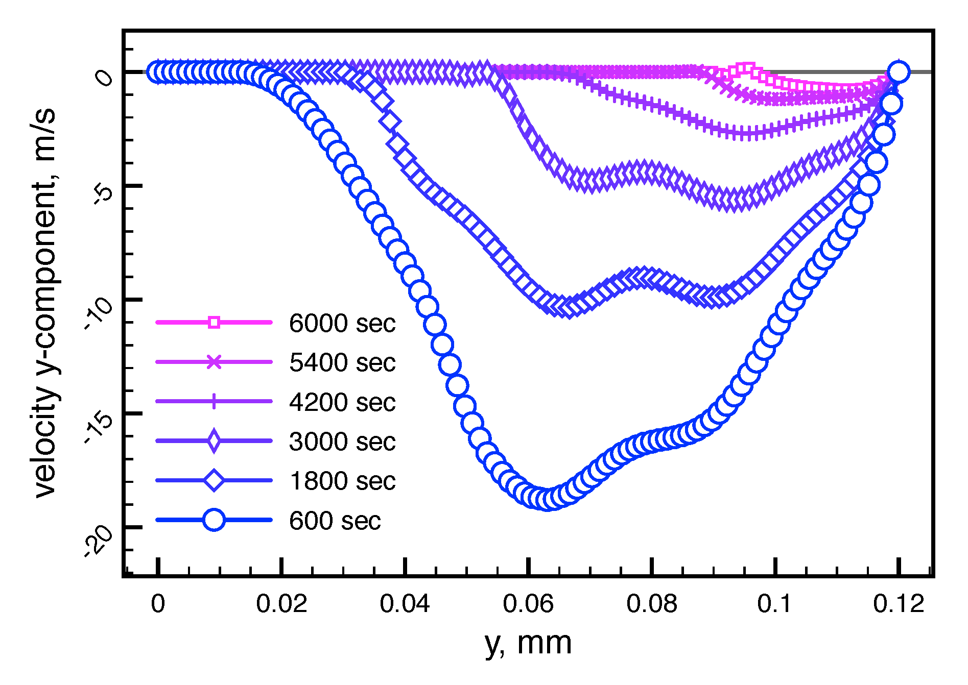
3.2.2. Spin-up Behaviour
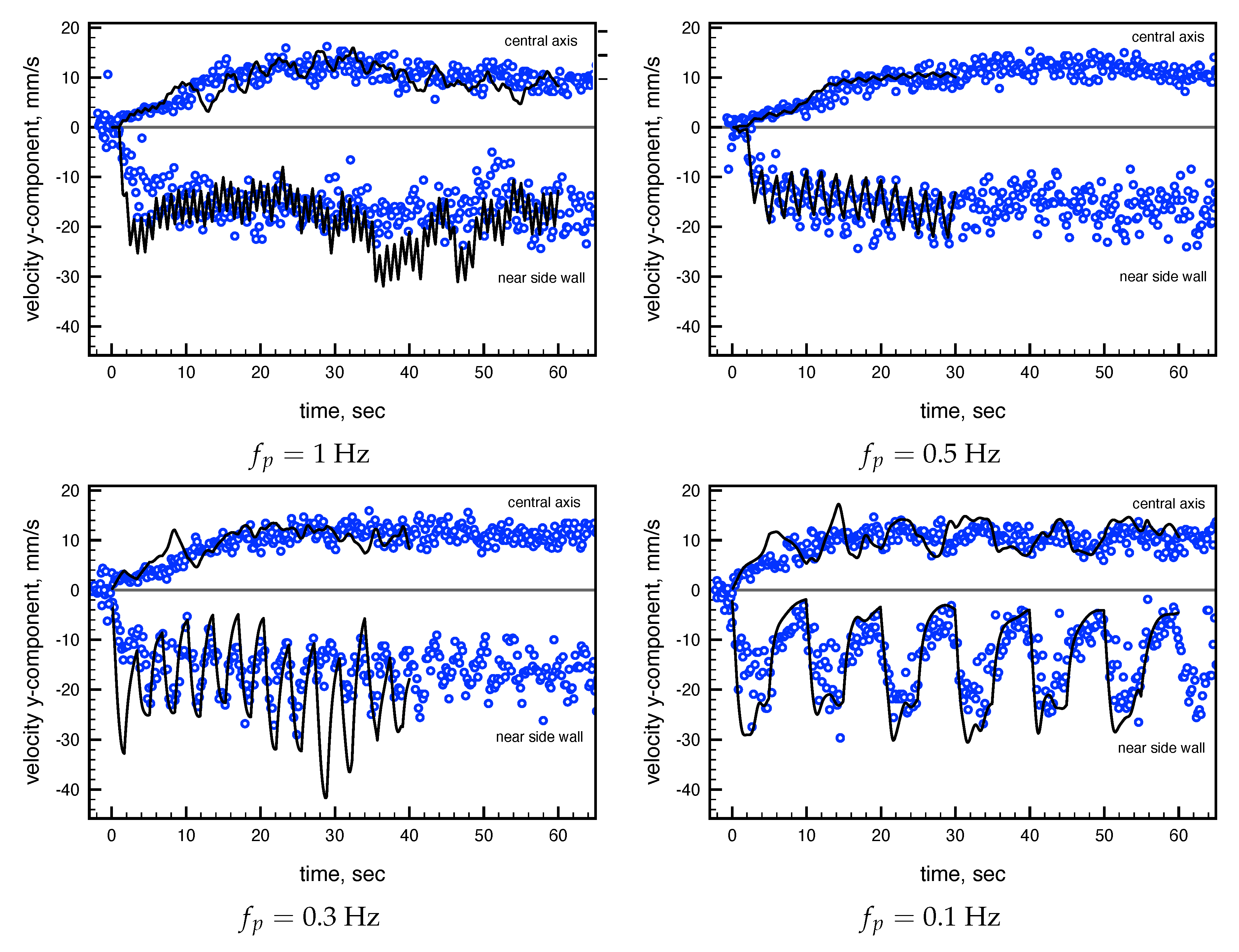
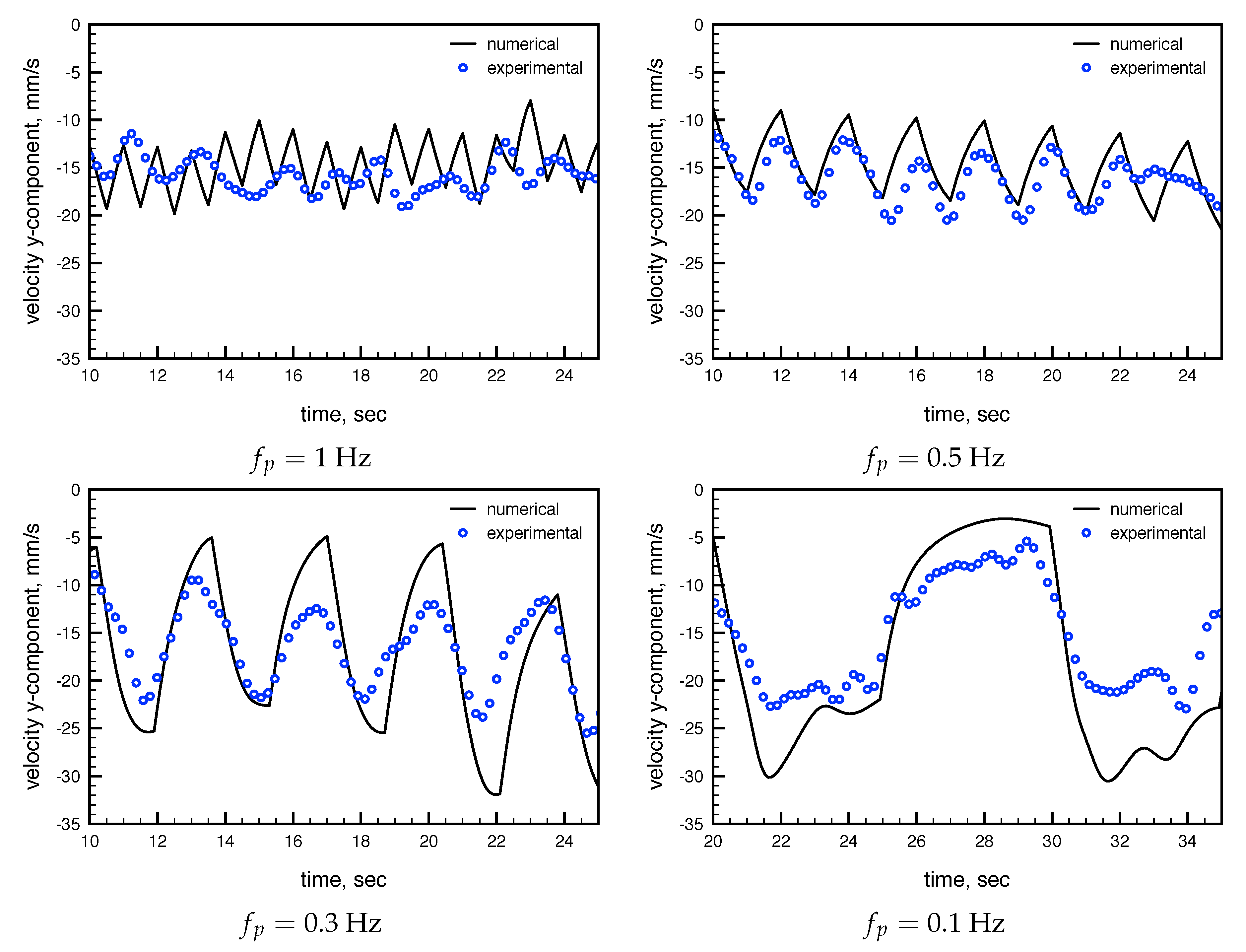
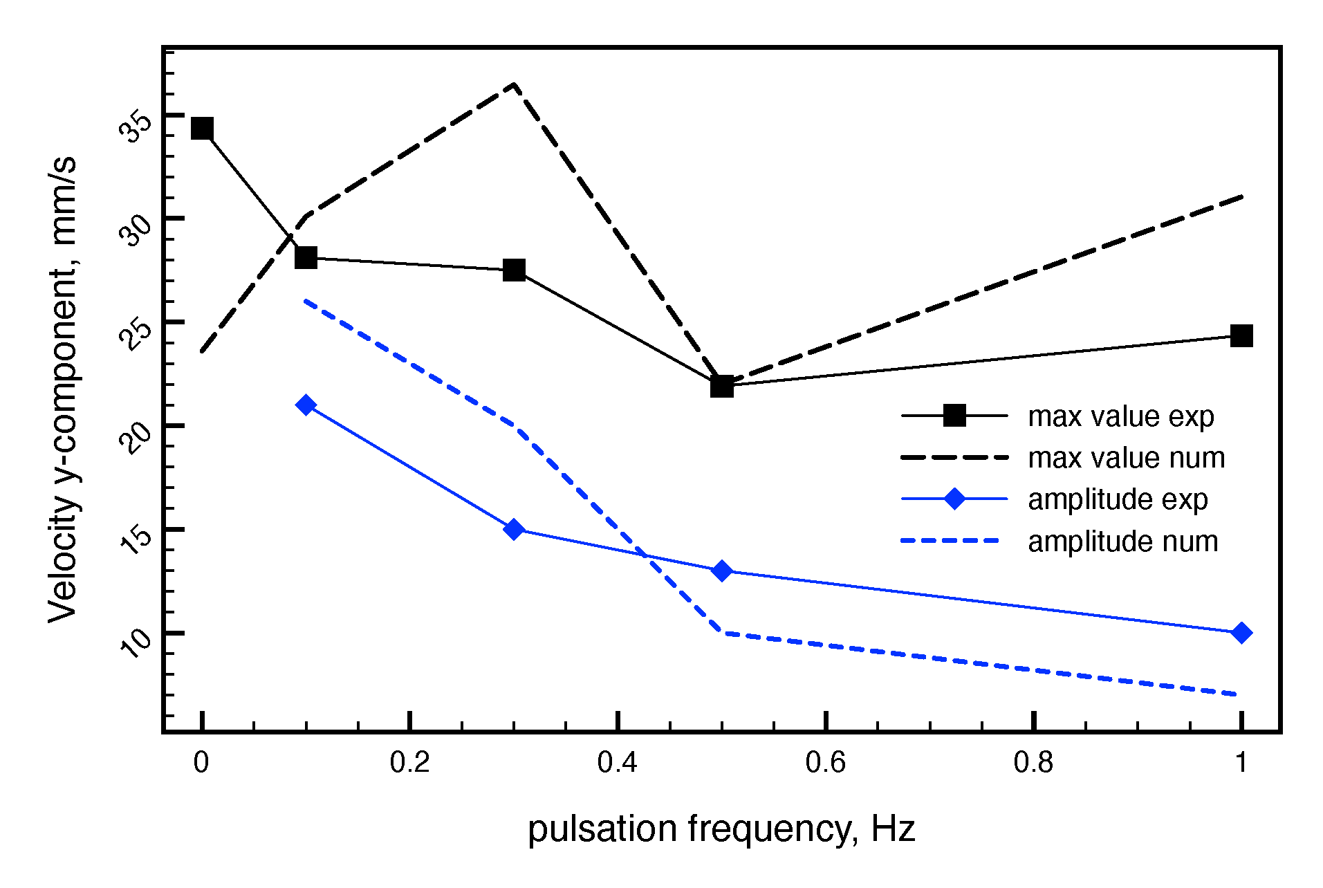
3.2.3. Pulsation Frequencies Analysis
4. Discussion
5. Conclusions
Supplementary Materials
Author Contributions
Funding
Acknowledgments
Conflicts of Interest
Abbreviations
| AMF | Alternating Magnetic Field |
| DOF | Degree of Freedom |
| EM | Electromagnetic |
| HD | Hydrodynamic |
| HMF | Helical Magnetic Field |
| LES | Large Eddy Simulation |
| MF | Magnetic Field |
| MHD | Magnetohydrodynamics |
| RANS | Reynolds-averaged Navier–Stokes |
| RMF | Rotating Magnetic Field |
| TMF | Travelling Magnetic Field |
Appendix A. Review on a Previous EM Stirring Studies
Appendix A.1. Previous EM Stirring of Melt in a Rectangular Cavity Investigations

| Author | Turbulence Model | Solidification, Method | Software | HD Mesh | Material and Size |
|---|---|---|---|---|---|
| Dadzis [27] | No turbulence model is used in flow calculation in the present study. Re = 1400 | GetDP, Elmer (thermal), OpenFOAM | A hexahedral grid with elements | Ga mm | |
| Kolesnichenko et al. [28,29,30] | SST | No | COMSOL (FEM) | 76,554 Hexahedral elements | GaSnZn mm |
| Ben David et al. [16,17,31] | laminar flow | Yes, C. Prakash, V.R. Voller approach | COMSOL | 10,469 elements with 60,000 DOF and 32,144 with 176 610 DOF [31] [16], 80,485 and the number of DOF was 73,550 for [17] | Ga (and GaInSn [17]) in a rectangular container of m. |
| Avnaim et al. [18,19,32] | The maximum Reynolds number is not greater than 2500. 3D Direct Numerical Simulation (DNS) | Yes, Multi-Domain method | COMSOL Multiphysics 5.0 (FEM) | 21,500 (120,000 DOF) Lagrange’s elements [18] and 50,000 (590,000 DOF) [19], 50,400 (275,110 DOF) for VOF method and 22,890 (708,420 DOF) for the MD modell [32]. | The gallium in cavity with the dimensions m. |
| Hachani et al. [14,20,33] | Realizable k- | A three-phase volume averaged equiaxed model | ANSYS FLUENT | grid comprising 100 × 60 × 15 mesh cells | Ga–In–Sn alloy m |
| Wang et al. [13,26] | 2D Theoretical model | No | Analytical | 2D Theoretical model | GaInSn m |
| Köppen et al. [10,34] | Exp. | Yes | Exp. | Exp. | m (two inductors) |
| Dzelme et al. [35,36] | DES and SST | No | ANSYS Classic or Elmer and OpenFOAM | 1.035M or 300 k elements in work [36] 37,500 elements in work [35] | gallium m |
| Oborin et al. [15] | 2D a turbulence model | No | OpenFOAM for velocity field and an analytical solution for the electromagnetic body force | control volumes | gallium alloy (Ga87.5%, Sn10.5%, Zn2.0%); = 24 cm, = 18 cm and h = 9.5 cm (asymmetric cavity) |
Appendix A.2. Previous Modulation/Pulsation of MF Studies
| Author and References | Type of the MF | Modulation Frequencies | Numerical/Experimental | Optimal Criteria |
|---|---|---|---|---|
| Eckert et al. [12,37] | RMF | 0.2; 0.475; 0.77 Hz for pulsed and 0.02; 0.08; 0.15; 0.2 Hz for reversed cases [12]. For solidification case 0.1, 0.2, 0.3, 0.35, and 0.45 Hz [37]. | Numerical (with solidification) and experimental | 0.15 Hz for max intensity of the secondary flow and 0.45 Hz for avoiding a segregation. |
| Wang X. et al. [13,26] | TMF | The investigated modulation frequencies are 6, 5, 4, 3, 2, 1, 0.5, 0.2, 0.1, and 0.05 Hz (reversed modulation) | Analytical and Experimental by UDV | The optimum modulation frequency that would allow saturation to be reached is where saturation time , a—the half-width of a cavity y, —the effective viscosity. |
| Räbiger et al. [38] | RMF | Pulsed modulation with time period of ranges 2–6 sec. and 10–30 sec. | Experimental by UDV | Dependences of the secondary now intensity on the duration of the pulse cycle for different RMF intensity are found. |
| Oborin et al. [15] | TMF | Reverse frequencies are 0.08; 0.1; 1; 1.25; 10.00 Hz | Numerical in a OpenFOAM and experimental by an ultrasonic Doppler velocimeter | Introduced the coefficient of heterogeneity: that is, through the relation between the standard deviation of the impurity concentration Ci at all n points in the cavity from the final impurity concentration after stirring (at a time t) and the same standard deviation at the initial time . The characteristic stirring time , which determines the time when the parameter decreases to is also estimated |
| Dropka et al. [39,40] | TMF | pulsed downward TMF of 0.5 and 0.05 Hz for different modulation strength and modulation amplitude. | Global 3D numerical analysis. Flow in the melt was described by model by ANSYS CFX 13.0 and Ansys Classic. | The radial temperature profiles in the middle of the melt for various modulated TMF flows with unmodulated TMF driven flow are compared. The most promising flow pattern in this study was obtained for sinusoidal on-off mode of TMF pulsing with Hz. Also the mass fraction dynamics are examinated |
| Musaeva et al. [11] | AMF | Pulsed Lorentz force was applied in a range of the modulation frequency of 0.05 Hz 1 Hz. | Numerical by the ANSYS Fluent software package using a Large Eddy Simulation (LES) turbulence model. | Pulsed AMF influence on the turbulent kinetic energy of the melt flow was investigated. To recognize the effect of the low-frequency pulsed Lorentz force on the melt mixing, a simulation of the temperature field homogenization was carried out. |
| Hachani et al. [14] | TMF | The electromagnetic force direction is periodically reversed. Electromagnetic force inversion frequency is equal to 0.125 Hz. Electromagnetic | Exp. (thermocouples; chemical method coupled with the Inductive Coupled Plasma technique and X-ray analysis) | The diffrent parameters was analayzed experimentally to estimate a TMF influence on solidification process: 1. Temperature field evolution. 2. Final metallographic structure and grain size. 3. Solute distribution. 4. Lead concentration distribution (macro- and mesosegregations) and the morphology of segregated channels. |
| Wang B. et al. [41] | HMF | reversed periodically modulation with frequencies Hz | Ultrasonic Doppler velocimetry (UDV, DOP 3010) was used to quantitatively measure the liquid metal flow. | The averaged axial and azimuthal velocities for various modulation frequencies with different aspect ratio of vessel are obtained. An optimal modulation frequency, under which the magnetic field could efficiently stir the solute at the solidification front, exists both in secondary and global axial flow (0.1 Hz and 0.625 Hz, respectively). |
| Musaeva et al. [10] | TMF | Pulsed modulation of 0.1, 0.3, 0.5, 1, 2 Hz | Experimental by neutron radiography | It has been experimentally proved that a flatter shape of the solidification front and the reduced irregularity of the solid/liquid surface can be obtained with the value closer to the characteristic frequency of melt circulation. |
| Losev et al. [28,42] | TMF | Reversed and pulsed modulation with period of 20, 30, 40, 50 sec (0,05–0,02 Hz) | Numerical by FEM in COMSOL and experimental by UDV measurement | Average flow velocity and its root mean square vs. TMF inductor supply current and TMF reverse modulation period was analysed. The dynamics of the crystallization front position are computed by wave-legth analysis. |
| Shvydkiy et al. [43,44] | TMF | Reversed and pulsed modulation | Numerical by COMSOL | A homogenization parameter of particles into the volume are implemented. Modulation is shown more effective stirring of particles in both pulsed and reversed cases. |
| Khripchenko et al. [45] | RMF and TMF | Reversed modulation with periods from 8, 16, 24 and 32 sec | Numerical by Ansys CFX and experimental | Several parameters were analyzed: Number of grains, Brinell hardness, specific kinetic energy. The analysis of the experimental results has indicated extrema on the curve, illustrating the grain size in the ingot structure, being dependent on the period of reversals of the rotating magnetic field. It is revealed that in the experimentally studied period of reverse pulsations of the rotating magnetic field the integral characteristics of hydrodynamic fields, such as the specific kinetic energy of a large-scale flow, the energy of turbulent pulsations, the kinetic energy of vertical motion, depend monotonically on the period. |
References
- Moffatt, H.K. Electromagnetic stirring. Phys. Fluids Fluid Dyn. 1991, 3, 1336–1343. [Google Scholar] [CrossRef]
- Rebei, F.; Sand, U.; J., E.; Hongliang, Y. A stirring history. ABB Rev. 2016, 3, 45–48. [Google Scholar]
- Timofeev, V.N.; Khatsayuk, M.Y. Theoretical Design Fundamentals for MHD Stirrers for Molten Metals. Magnetohydrodynamics 2016, 52, 495–506. [Google Scholar]
- Dadzis, K. Modeling of directional solidification of multicrystalline silicon in a traveling magneticfield. Ph.D. Thesis, Technischen Universitat Bergakademie Freiberg Genehmigte, Freiberg, Germany, 2012. [Google Scholar]
- Molokov, S.; Moreau, R.; Moffatt, K. Magnetohydrodynamics; Springer: Dordrecht, The Netherlands, 2007. [Google Scholar] [CrossRef]
- Eskin, D.G.; Mi, J. (Eds.) Solidification Processing of Metallic Alloys Under External Fields; Springer: Cham, Seitzerland, 2018; Volume 273. [Google Scholar] [CrossRef]
- Noeppel, A.; Ciobanas, A.; Wang, X.D.; Zaidat, K.; Mangelinck, N.; Budenkova, O.; Weiss, A.; Zimmermann, G.; Fautrelle, Y. Influence of Forced/Natural Convection on Segregation During the Directional Solidification of Al-Based Binary Alloys. Metall. Mater. Trans. B 2010, 41, 193–208. [Google Scholar] [CrossRef]
- Eckert, S.; Nikrityuk, P.A.; Willers, B.; Räbiger, D.; Shevchenko, N.; Neumann-Heyme, H.; Travnikov, V.; Odenbach, S.; Voigt, A.; Eckert, K. Electromagnetic melt flow control during solidification of metallic alloys. Eur. Phys. J. Spec. Top. 2013, 220, 123–137. [Google Scholar] [CrossRef]
- Mikolajczak, P. Microstructural Evolution in AlMgSi Alloys during Solidification under Electromagnetic Stirring. Metals 2017, 7, 89. [Google Scholar] [CrossRef]
- Musaeva, D.; Baake, E.; Koppen, A.; Vontobel, P. Application of neutron radiography for in-situ visualization of gallium solidification in travelling magnetic field. Magnetohydrodynamics 2017, 53, 583–593. [Google Scholar]
- Musaeva, D.; Ilin, V.; Baake, E.; Geža, V. Numerical simulation of the melt flow in an induction crucible furnace driven by a Lorentz force pulsed at low frequency. Magnetohydrodynamics 2015, 51, 771–784. [Google Scholar]
- Eckert, S.; Nikrityuk, P.A.; Räbiger, D.; Eckert, K.; Gerbeth, G. Efficient melt stirring using pulse sequences of a rotating magnetic field: Part I. flow field in a liquid metal column. Metall. Mater. Trans. B 2007, 38, 977–988. [Google Scholar] [CrossRef]
- Wang, X.; Fautrelle, Y.; Etay, J.; Moreau, R. A Periodically Reversed Flow Driven by a Modulated Traveling Magnetic Field: Part I. Experiments with GaInSn. Metall. Mater. Trans. B 2008, 40, 82. [Google Scholar] [CrossRef]
- Hachani, L.; Zaidat, K.; Fautrelle, Y. Experimental study of the solidification of Sn-10 wt.%Pb alloy under different forced convection in benchmark experiment. Int. J. Heat Mass Transf. 2015, 85, 438–454. [Google Scholar] [CrossRef]
- Oborin, P.; Khripchenko, S.; Golbraikh, E. Influence of conventional and reverse travelling magnetic fields on liquid metal stirring in an asymmetric cavity. Magnetohydrodynamics 2014, 50, 291–302. [Google Scholar] [CrossRef]
- Ben-David, O.; Levy, A.; Mikhailovich, B.; Azulay, A. Impact of rotating permanent magnets on gallium melting in an orthogonal container. Int. J. Heat Mass Transf. 2015, 81, 373–382. [Google Scholar] [CrossRef]
- Ben-David, O.; Levy, A.; Mikhailovich, B.; Avnaim, M.; Azulay, A. Impact of traveling permanent magnets on low temperature metal melting in a cuboid. Int. J. Heat Mass Transf. 2016, 99, 882–894. [Google Scholar] [CrossRef]
- Avnaim, M.H.; Mikhailovich, B.; Azulay, A.; Levy, A. Numerical and experimental study of the traveling magnetic field effect on the horizontal solidification in a rectangular cavity part 1: Liquid metal flow under the TMF impact. Int. J. Heat Fluid Flow 2018, 69, 23–32. [Google Scholar] [CrossRef]
- Avnaim, M.H.; Mikhailovich, B.; Azulay, A.; Levy, A. Numerical and experimental study of the traveling magnetic field effect on the horizontal solidification in a rectangular cavity part 2: Acting forces ratio and solidification parameters. Int. J. Heat Fluid Flow 2018, 69, 9–22. [Google Scholar] [CrossRef]
- Wang, T.; Hachani, L.; Fautrelle, Y.; Delannoy, Y.; Wang, E.; Wang, X.; Budenkova, O. Numerical modeling of a benchmark experiment on equiaxed solidification of a Sn–Pb alloy with electromagnetic stirring and natural convection. Int. J. Heat Mass Transf. 2020, 151, 119414. [Google Scholar] [CrossRef]
- Brent, A.D.; Voller, V.R.; Reid, K.J. Enthalpy-porosity technique for modeling convection-diffusion phase change: Application to the melting of a pure metal. Numer. Heat Transf. 1988, 13, 297–318. [Google Scholar] [CrossRef]
- Dobosz, A.; Plevachuk, Y.; Sklyarchuk, V.; Sokoliuk, B.; Gancarz, T. Thermophysical properties of the liquid Ga–Sn–Zn eutectic alloy. Fluid Phase Equilibria 2018, 465, 1–9. [Google Scholar] [CrossRef]
- Umbrashko, A.; Baake, E.; Nacke, B.; Jakovics, A. Modeling of the turbulent flow in induction furnaces. Metall. Mater. Trans. B 2006, 37, 831–838. [Google Scholar] [CrossRef]
- Galindo, V.; Nauber, R.; Räbiger, D.; Franke, S.; Beyer, H.; Büttner, L.; Czarske, J.; Eckert, S. Instabilities and spin-up behaviour of a rotating magnetic field driven flow in a rectangular cavity. Phys. Fluids 2017, 29, 114104. [Google Scholar] [CrossRef]
- Räbiger, D.; Eckert, S.; Gerbeth, G. Measurements of an unsteady liquid metal flow during spin-up driven by a rotating magnetic field. Exp. Fluids 2010, 48, 233–244. [Google Scholar] [CrossRef]
- Wang, X.; Moreau, R.; Etay, J.; Fautrelle, Y. A Periodically Reversed Flow Driven by a Modulated Traveling Magnetic Field: Part II. Theoretical Model. Metall. Mater. Trans. B 2009, 40, 104–113. [Google Scholar] [CrossRef]
- Dadzis, K.; Lukin, G.; Meier, D.; Bönisch, P.; Sylla, L.; Pätzold, O. Directional melting and solidi fi cation of gallium in a traveling magnetic fi eld as a model experiment for silicon processes. J. Cryst. Growth 2016, 445, 90–100. [Google Scholar] [CrossRef]
- Losev, G.; Shvydkiy, E.; Sokolov, I.; Pavlinov, A.; Kolesnichenko, I. Effective stirring of liquid metal by a modulated travelling magnetic field. Magnetohydrodynamics 2019, 55, 107–114. [Google Scholar]
- Losev, G.L.; Kolesnichenko, I.V.; Khalilov, R.I. Control of the metal crystallization process by the modulated traveling magnetic field. J. Phys. Conf. Ser. 2018, 1128, 012051. [Google Scholar] [CrossRef]
- Shvydkiy, E.; Kolesnichenko, I.; Khalilov, R.; Pavlinov, A.; Losev, G. Effect of travelling magnetic field inductor characteristics on the liquid metal flow in a rectangular cell. IOP Conf. Ser. Mater. Sci. Eng. 2018, 424, 012012. [Google Scholar] [CrossRef]
- Ben-David, O.; Levy, A.; Mikhailovich, B.; Azulay, A. 3D numerical and experimental study of gallium melting in a rectangular container. Int. J. Heat Mass Transf. 2013, 67, 260–271. [Google Scholar] [CrossRef]
- Avnaim, M.H.; Levy, A.; Mikhailovich, B.; Ben-David, O.; Azulay, A. Comparison of Three-Dimensional Multidomain and Single-Domain Models for the Horizontal Solidification Problem. J. Heat Transf. 2016, 138. [Google Scholar] [CrossRef]
- Zaidat, K.; Sari, I.; Boumaaza, A.; Abdelhakem, A.; Hachani, L.; Fautrelle, Y. Experimental investigation of the effect of travelling magnetic field on the CET in Sn-10wt.%Pb alloy. In Proceedings of the IOP Conference Series: Materials Science and Engineering, Hyogo, Japan, 14–18 October 2018. [Google Scholar] [CrossRef]
- Koppen, D.; Baake, E.; Gerstein, G.; Mrówka-Nowotnik, G.; Jarczyk, G. Resonant pulsed electromagnetic stirring of melt for effective grain fragmentation. In Proceedings of the IOP Conference Series: Materials Science and Engineering, Hyogo, Japan, 14–18 October 2018. [Google Scholar] [CrossRef]
- Dzelme, V.; Jakovics, A.; Vencels, J.; Köppen, D.; Baake, E. Numerical and experimental study of liquid metal stirring by rotating permanent magnets. In Proceedings of the IOP Conference Series: Materials Science and Engineering, Hyogo, Japan, 14–18 October 2018. [Google Scholar] [CrossRef]
- Dzelme, V.; Ščepanskis, M.; Geža, V.; Jakovičs, A.; Sarma, M. Modelling of liquid metal stirring induced by four counter-rotating permanent magnets. Magnetohydrodynamics 2016, 52, 461–470. [Google Scholar]
- Willers, B.; Eckert, S.; Nikrityuk, P.A.; Räbiger, D.; Dong, J.; Eckert, K.; Gerbeth, G. Efficient Melt Stirring Using Pulse Sequences of a Rotating Magnetic Field: Part II. Application to Solidification of Al-Si Alloys. Metall. Mater. Trans. B 2008, 39, 304–316. [Google Scholar] [CrossRef]
- Räbiger, D.; Eckert, S.; Gerbeth, G.; Franke, S.; Czarske, J. Flow structures arising from melt stirring by means of modulated rotating magnetic fields. Magnetohydrodynamics 2012, 48, 213–220. [Google Scholar] [CrossRef]
- Dropka, N.; Frank-Rotsch, C. Enhanced VGF-GaAs growth using pulsed unidirectional TMF. J. Cryst. Growth 2014, 386, 146–153. [Google Scholar] [CrossRef]
- Dropka, N.; Frank-Rotsch, C. Enhanced VGF growth of singleand multi-crystalline semiconductors using pulsed TMF. Magnetohydrodynamics 2015, 51, 149–156. [Google Scholar] [CrossRef]
- Wang, B.; Wang, X.; Etay, J.; Na, X.; Zhang, X.; Fautrelle, Y. Flow Driven by an Archimedean Helical Permanent Magnetic Field. Part I: Flow Patterns and Their Transitions. Metall. Mater. Trans. B 2016, 47, 1369–1377. [Google Scholar] [CrossRef]
- Losev, G.; Pavlinov, A.; Shvydkiy, E.; Sokolov, I.; Kolesnichenko, I. Stirring flow of liquid metal generating by low-frequency modulated traveling magnetic field in rectangular cell. In Proceedings of the IOP Conference Series: Materials Science and Engineering, Perm, Russian, 18–22 February 2019. [Google Scholar] [CrossRef]
- Shvydkiy, E.; Bolotin, K.; Sokolov, I. 3D simulation of particle transport in the double-sided travelling magnetic field stirrer. Magnetohydrodynamics 2019, 55, 185–192. [Google Scholar]
- Shvydkii, E.L.; Bychkov, S.A.; Zakharov, V.V.; Sokolov, I.V.; Tarasov, F.E. Impurity Distribution in a Two-Sided Electromagnetic Stirrer. Russ. Metall. (Metally) 2019, 2019, 570–575. [Google Scholar] [CrossRef]
- Khripchenko, S.; Denisov, S.; Dolgikh, V.; Shestakov, A.; Siraev, R. Structure of solidified aluminum melt in crucibles of circularandsquare cross-sections in reverse regimes of rotating magnetic field. Magnetohydrodynamics 2019, 55, 437–445. [Google Scholar] [CrossRef]


| Property | Value | Units | ||
|---|---|---|---|---|
| Ga (solid) | density | 5910 | kg/m | |
| k | thermal conductivity | W/m ·K | ||
| specific heat | 396 J/kg · K | |||
| Ga (liquid) | Solidification temperature | 303 | K | |
| density | kg/m | |||
| k | thermal conductivity | W/m ·K | ||
| specific heat | 407 | J/kg ·K | ||
| dynamic viscosity | kg/m ·s | |||
| latent heat | 80200 | J/kg· K | ||
| electrical conductivity | S/m |
© 2020 by the authors. Licensee MDPI, Basel, Switzerland. This article is an open access article distributed under the terms and conditions of the Creative Commons Attribution (CC BY) license (http://creativecommons.org/licenses/by/4.0/).
Share and Cite
Shvydkiy, E.; Baake, E.; Köppen, D. Liquid Metal Flow Under Traveling Magnetic Field—Solidification Simulation and Pulsating Flow Analysis. Metals 2020, 10, 532. https://doi.org/10.3390/met10040532
Shvydkiy E, Baake E, Köppen D. Liquid Metal Flow Under Traveling Magnetic Field—Solidification Simulation and Pulsating Flow Analysis. Metals. 2020; 10(4):532. https://doi.org/10.3390/met10040532
Chicago/Turabian StyleShvydkiy, Evgeniy, Egbert Baake, and Diana Köppen. 2020. "Liquid Metal Flow Under Traveling Magnetic Field—Solidification Simulation and Pulsating Flow Analysis" Metals 10, no. 4: 532. https://doi.org/10.3390/met10040532
APA StyleShvydkiy, E., Baake, E., & Köppen, D. (2020). Liquid Metal Flow Under Traveling Magnetic Field—Solidification Simulation and Pulsating Flow Analysis. Metals, 10(4), 532. https://doi.org/10.3390/met10040532