The Angular Velocity as a Function of the Radius in Molten Ga75In25 Alloy Stirred Using a Rotation Magnetic Field

Abstract

The simulation of the solidification of alloys (like steel or aluminium alloys), which is carried out by using the melt flow induced by a rotation magnetic field (RMF), needs the correct angular velocity vs. the radius function of the melt. Because it is impossible to directly obtain information about the melt flow from industrial casting, this information can only be obtained from well-monitored experiments using low-melting-point metals or alloys (e.g., Hg, Ga, GaIn, and GaInSn). In this work, we first summarized the measuring methods that are suitable for determining this function and analysed their advantages and disadvantages. All of them disturb, to some degree, the melt flow, except for the Pressure Compensation Method (PCM); therefore, this method was used in the experiments. Closed TEFLON crucibles with a 60 mm length and 12.5 mm radius and Ga75wt%In25wt% alloy was used. The angular velocity (ω) was calculated from the compensation pressure measured at r = 5, 7.5, 10, and 12.5 mm in the 0–90 mT range of magnetic induction, B. Based on the ω(B, r) dataset, a suitable ω(B, r) function was determined for the simulation.

1. Introduction

The aim of simulating the solidification of alloys (like the semicontinuous casting of aluminium alloys or the continuous casting of steels) is to produce a tool that can integrate the planning of the process parameters, which can guarantee a suitable microstructure and good mechanical properties [1,2,3,4,5]. In the continuous casting of steel, magnetic stirring is used worldwide to obtain a microstructure without a columnar zone and central macrosegregation extending across the centre equiaxed zone, refine the grain size, minimise the shrinkage porosity and macrosegregation, and improve the surface quality [6,7,8,9,10,11,12,13,14,15,16,17,18]. The magnetic induction causes a melt flow, and its simulation is complicated and needs correct data, like the ω(B, r) function. It is known that obtaining information about the melt flow from industrial casting is impossible, so we must conduct some cold experiments with well-monitored parameters (like Hg, Ga, GaIn, and GaInSn alloys) [19,20,21,22,23,24,25,26,27]. Because only very little correctly measured data for the ω(B, r) function can be found in the literature [21,22,23,25,28,29,30,31,32,33,34,35], any previous simulations of the melt flow induced by an RMF ignored the function to solve the problem mentioned above [6,7,8,9,10,11]. After analysing the known methods used to determine the ω(B, r) function, the most suitable method, namely the Press Compensation Method (PCM), was chosen. This study aims to provide a correct dataset for validating the ω(B, r) function before this simulation is used in industrial processes.

2. Measuring Methods Used

Four different methods are given in the literature to obtain information about the angular velocity of the melt induced by a Rotating Magnetic Field (RMF); these methods are as follows:

(1) Investigate the form of the free surface, (2) measure the angular velocity using a “turbine”, which is immersed in the melt, (3) measure the angular velocity by using a conductive anemometer with its own magnetic field, and (4) take a pressure difference measurement. All four methods have some advantages and disadvantages.

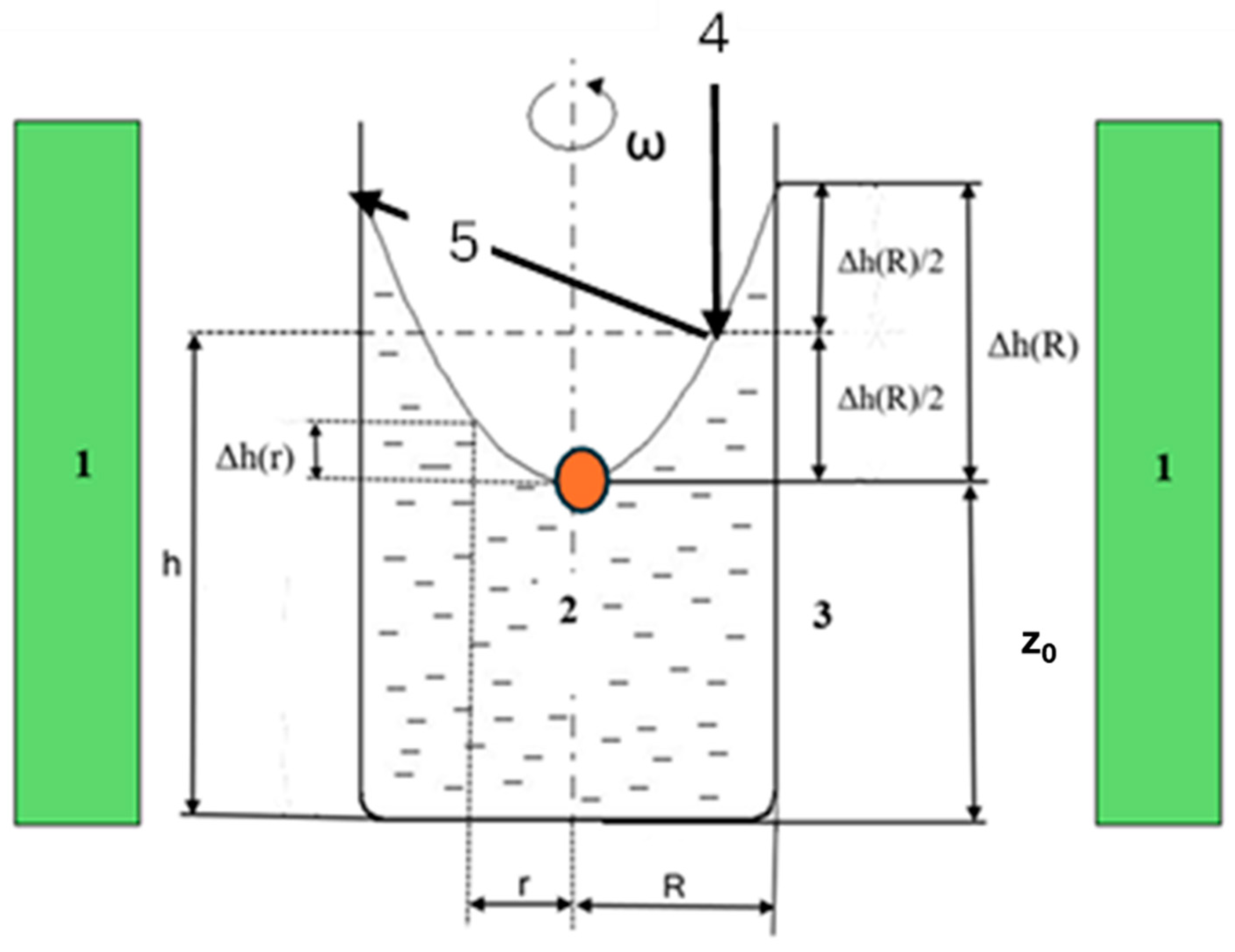
ad.1. Investigate the form of the free surface

The form of the free surface of the rotated melt is a paraboloid if the Lorence Force (F_.L.), which produces the rotation, is constant along the radius; then, the liquid’s viscosity and the wall friction can be negligible, and the aspect ratio (h/2R) can be higher than 6. In this case, the angular velocity (ω) is constant along the radius. To measure the fall in the original surface in the centre of the paraboloid (red circle and Δh/2 in Figure 1) [31], the calculation can be carried out as follows:

$$\mathsf{\omega }\left(\mathrm{R}\right)={\left(2\mathrm{g}\mathsf{\Delta }\mathrm{h}\left(\mathrm{R}\right)\right)}^{0.5}/\mathrm{R}=\mathsf{\omega }\left(\mathrm{r}\right)={\left(2\mathrm{g}\mathsf{\Delta }\mathrm{h}\left(\mathrm{r}\right)\right)}^{0.5}/\mathrm{r}$$

(1)

where g is the gravitation constant, R is the crucible’s radius, and 0 < r < R.

If the F_.L. is not constant along the radius (the magnetic induction is not constant), the wall friction and/or the effect of the viscosity cannot be negligible, and the form of the free surface is not a paraboloid, so $\mathsf{\omega }\left(\mathrm{R}\right)\ne \mathsf{\omega }\left(\mathrm{r}\right).$

The Δh(R) value is measured mechanically or with the use of laser rays. The latter method is more precise. The Δh(r) value cannot be measured using laser rays (4) because the backscattered laser ray (5) is absorbed in the crucible wall (see Figure 1). So, only the $\mathsf{\omega }\left(\mathrm{R}\right)$ value is measurable using a laser.

Advantage:

(i)

Conducting the measurement is simple.

Disadvantages:

(i)

It is not too easy to find the deepest point.

(ii)

Because the viscosity of the melt and the wall friction are usually not negligible, the form of the free surface is not exactly a paraboloid (i.e., there is a potential formation of vortexes), so ω changes with r.

(iii)

The ω(B, r) function is not practically measurable.

ad.2. Measure the angular velocity by using a “turbine”

By immersing a so-called “turbine” into the rotated melt and measuring the revolution number (Rpm, n) of the axis of the “turbine”, the angular velocity is calculated as follows:

$$\mathsf{\omega }=2\mathsf{\pi }\mathrm{n}/60$$

(2)

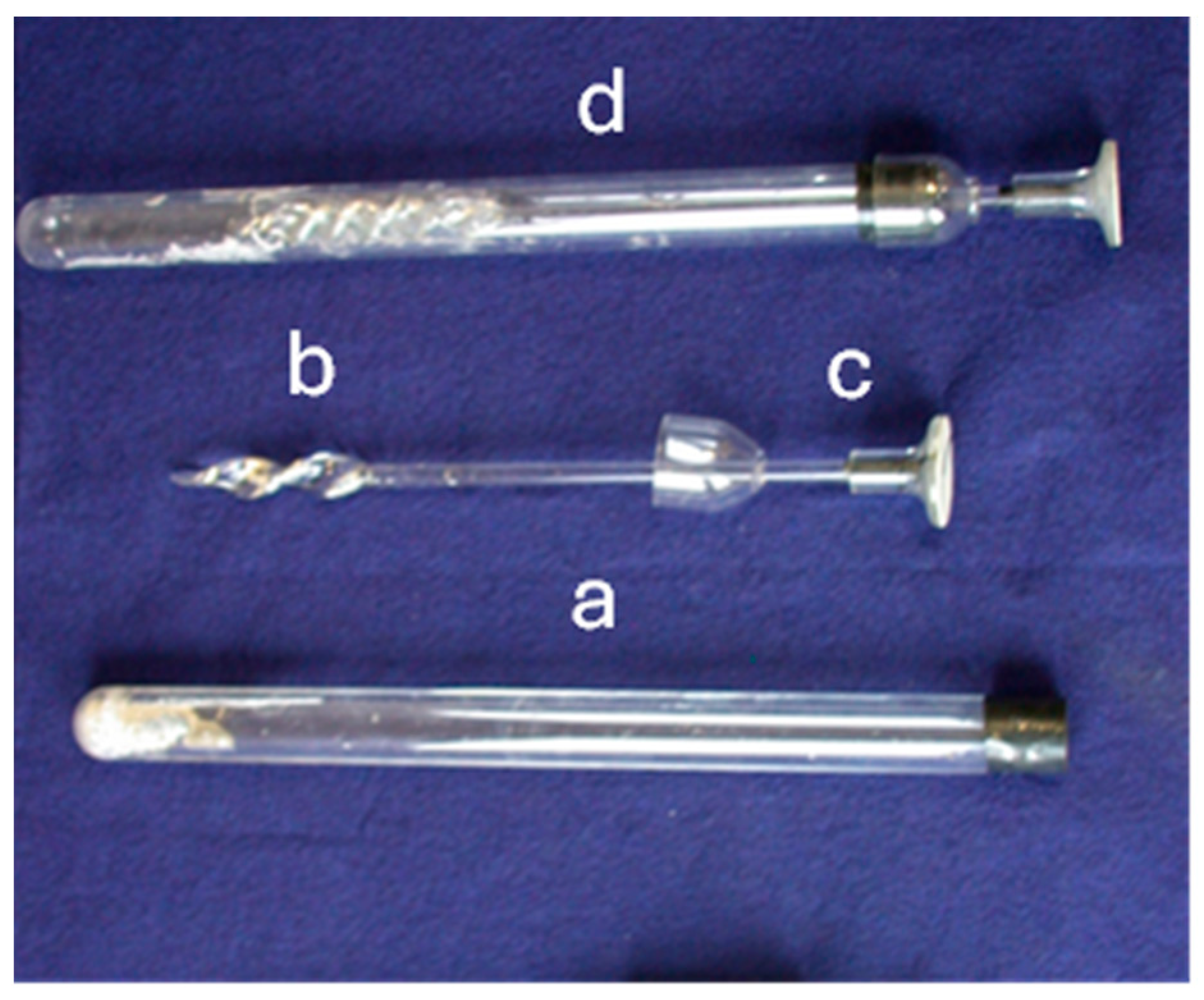
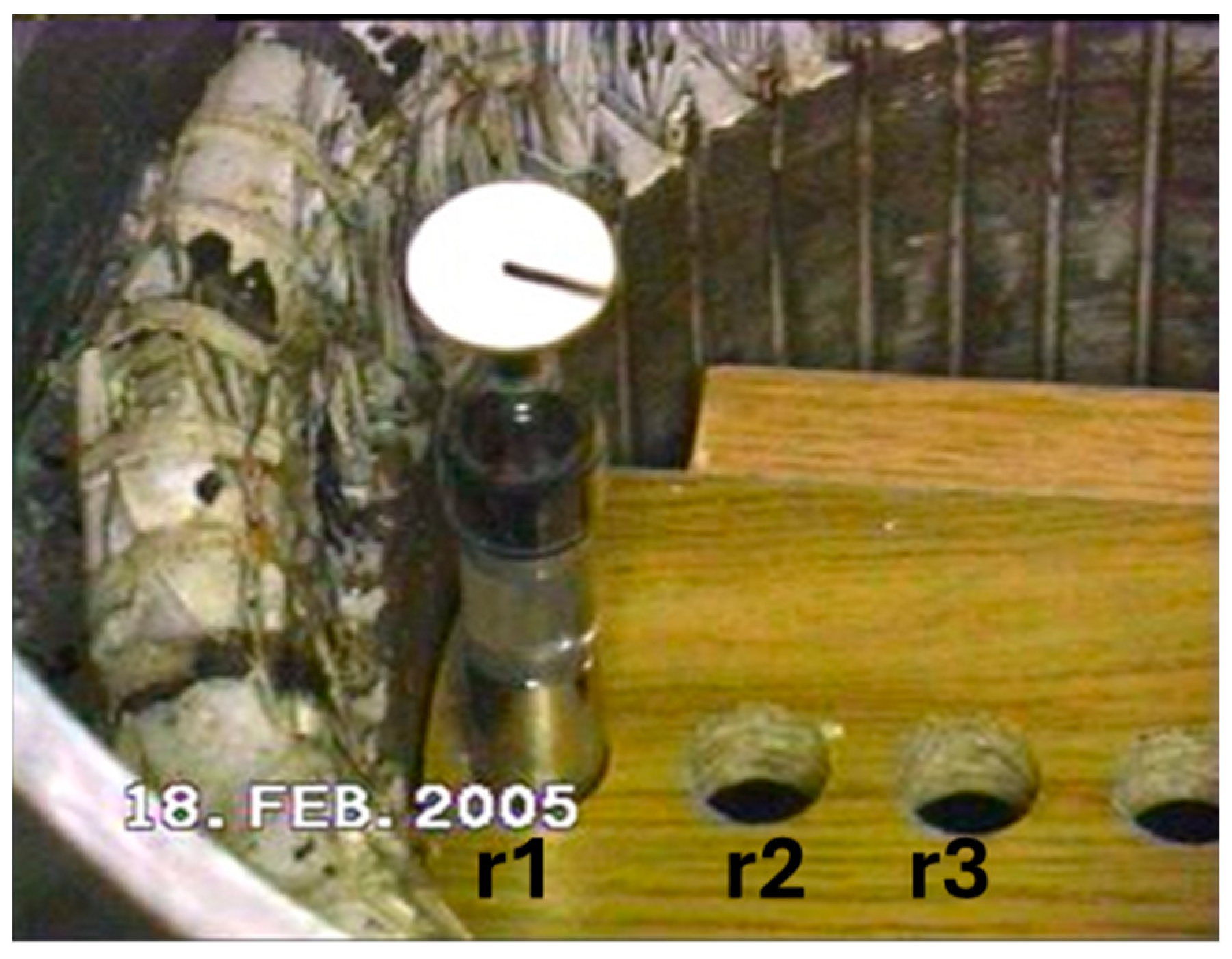
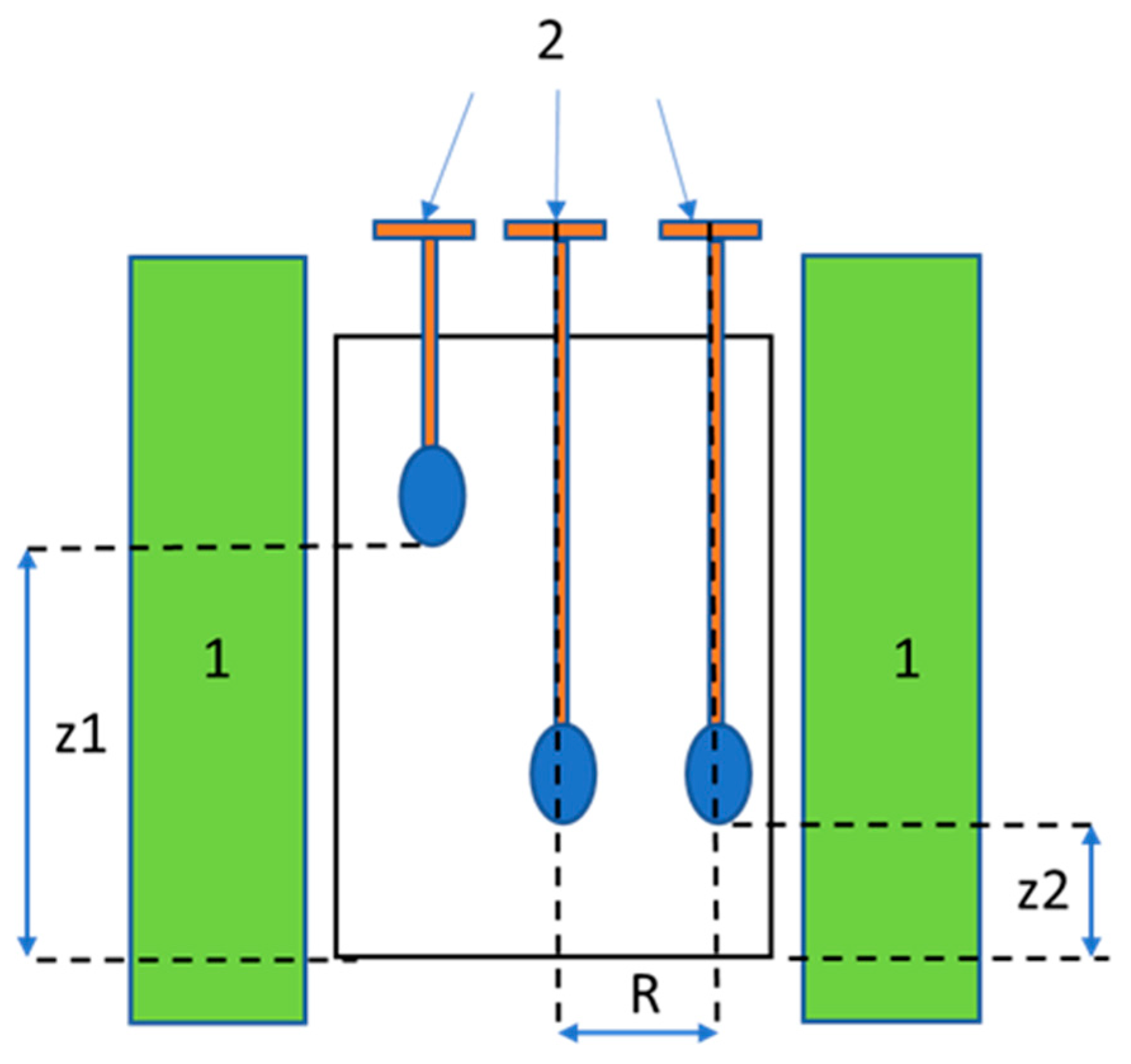
In [23], a “turbine” was made that consisted of a glass ampoule (a) containing liquid Ga and a “turbine blade” (b) formed at the higher end of a glass shaft that was immersed into liquid Ga (version A). The bearing of the “shaft + turbine blade” was placed into the cap, closing the top of the glass ampoule (Figure 2). The rotating liquid Ga rotated the shaft. The Rpm of the turbine was determined by evaluating the video film taken of the marked disc located on the upper part of the shaft. (Figure 3). By placing the small turbine into the holes, which are the different distances from the wall of the inductor, the ω value can be measured as a function of r. In a bigger crucible (Figure 4), the turbine blade could be placed at a different radius r (r1, r2 and r3) or height, so ω can be mapped in the hole crucible.

In [21], another type of “turbine” was used (Figure 5) (version B). One turbine consists of 8 blue rods (turbine blade, 2) fixed on a wheel and (5) immersed in the mercury melt in a glass crucible (4). The radius (R) of the fixing wheel is changeable, so the Rpm is measurable at a different distance from the centre. The rotation of the shaft (3) is used to measure the Rpm.

Advantages:

(i)

It is a mechanical facility that is not too complicated;

(ii)

It can map the ω value in the whole crucible;

(iii)

It can spectacularly demonstrate the rotation of the melt.

Disadvantages:

(i)

If the torque caused by the friction force between the cover of the crucible (6) and the shaft (3) is too high compared with the torque caused by the Lorenz Force (especially B < 15 mT), the measured ω would be smaller than the real one.

(ii)

The turbine blades (version A) or the rods (version B) disturb the flow, especially in the case of a relatively high magnetic induction (B > 100 mT), when a vortex can form near them.

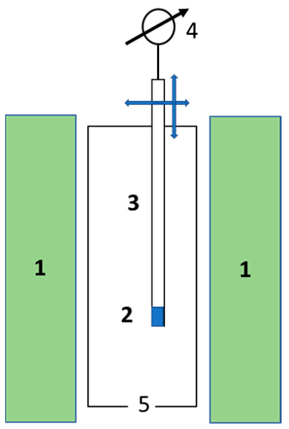
ad.3. Perform the measurement using a conductive anemometer with its own magnetic field

The conductive anemometer is made from a thin ceramic tube (3 in Figure 6) [22]. A longitudinally magnetised permanent magnet is mounted at one end of the tube (2). Electrodes made from copper wire are mounted at the two opposite sides of the magnet and aligned along its axis. The induced voltage is measured using a nano-voltmeter (4). The ceramic tube is fixed in the holder of the traverse gear and can move along the radial and axial (blue arrows). The facility must calibrate with the mechanically rotated melt with different angular velocities.

Advantages:

(i)

Conducting the measurement is simple.

(ii)

Moving the anemometer into radial and axial directions could allow the ω value to be mapped in the whole crucible, including the ω(B, r) function.

Disadvantages:

(i)

The ceramic tube mechanically disturbs the melt flow (the vortex near the ceramic tube) and the permanent magnet magnetically disturbs the melt flow.

(ii)

Calibrating the facility is complicated.

(iii)

It can only be used at a small magnetic induction (B ≤ 5 mT).

ad.4 Pressure difference measurement

The pressure changes if the melt is rotated in a closed crucible without a free surface. A higher pressure corresponds to a larger radius and larger velocity. This phenomenon can be used to determine the Rpm of the rotating melt stirred using an RMF. The pressure difference, Δp, related to the pressure prevailing at the axis of rotation, can be calculated from the velocity differences present at any place with a radius of r. The peripheral speed was zero at the sample axis (r = 0), whereas the maximum value was at the crucible wall (r = R).

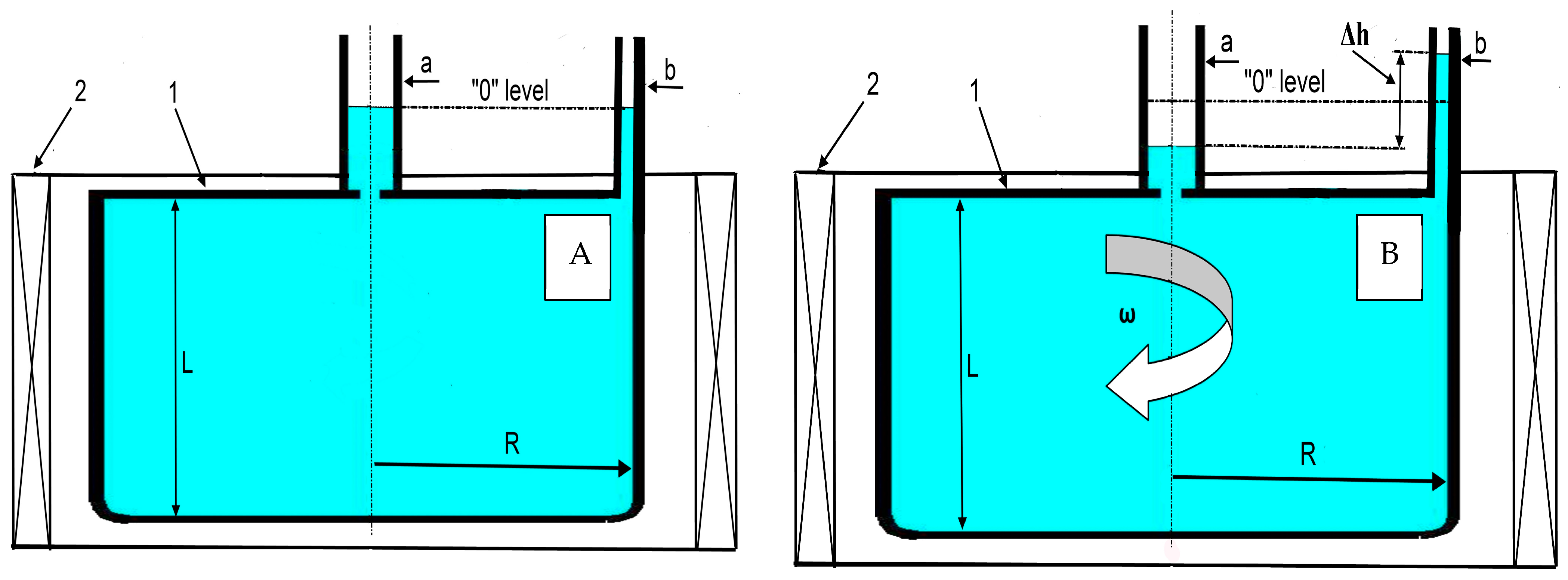
The crucible is closed with two gauges connections to measure the pressure at r = R [24]. The gauges at the tank’s axis (r = 0) and periphery (R) are labelled, respectively, “a” and “b” in Figure 7A. The two gauges connections and crucible are a “communication vessel”. The melt level is the same as that at the gauge connections if the RMF inductor is not operated. Moreover, the atmospheric pressure is identical in the so-called “stationary-level” or “0-level” gauge connections.

A level difference of Δh developed between the melt levels in the “a” and “b” gauge connections when the melt was rotated (stirred) using the RMF inductor (Figure 7B). The ρgΔh metal-static pressure of the melt column is in equilibrium with the pressure difference (Δp) developed between the axis and periphery of the crucible. If the free surface of the melt is at atmospheric pressure in the gauge connections,

$$∆\mathrm{p}\left(\mathrm{R}\right)=\mathsf{\rho }[{\mathrm{v}\left(\mathrm{R}\right)]}^2/2=\mathsf{\rho }{\mathsf{\omega }}^2{\mathrm{R}}^2/2$$

(3)

The azimuthal (v) and angular velocity (ω) of the metallic column can be calculated as follows:

$$\mathrm{v}={\left(2\mathsf{\Delta }\mathrm{p}\right(\mathrm{R})/\mathsf{\rho })}^{0.5}$$

(4)

and

$$\mathsf{\omega }={\left(2\mathsf{\Delta }\mathrm{p}\right(\mathrm{R})/\mathsf{\rho })}^{0.5}/\mathrm{R}$$

(5)

The Δp can be measured using two methods: (a) using a manometer and (b) with pressure compensation.

(a)

Measuring using a manometer [22]

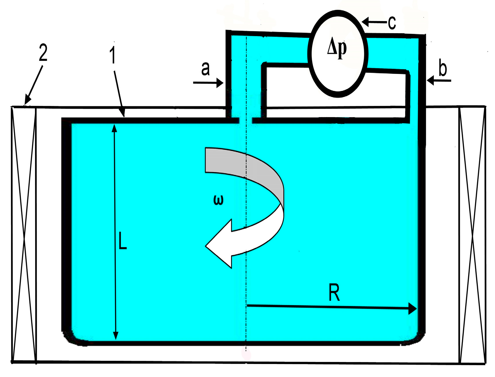
A differential manometer is placed between the two measuring connectors and directly used to measure the Δp (Figure 8).

Advantages:

(i)

During the measurement, nothing in the melt can disturb the melt flow.

Disadvantages:

(i)

There must not be air in the measuring system because it interferes with the measurement.

(ii)

The differential manometer can be damaged by metallic melt.

(iii)

The ω(B, r) function cannot be measured in this form.

(b)

Pressure Compensation Method (PCM)

The Δp = ρgΔh differential pressure is compensated by an external p_comp = ρgΔh pressure produced by a compressor at measurement gauge “b”; the “0” level is restored at both gauges “a” and “b” (Figure 9) [31,32,33].

$${\mathsf{\omega }=(2{\mathrm{p}}_{\mathrm{c}\mathrm{o}\mathrm{m}\mathrm{p}}/\mathsf{\rho })}^{0.5}/\mathrm{R}$$

(6)

Advantages:

(i)

During the measurement, there is nothing in the melt that can disturb the melt flow.

(ii)

The ω is measurable in an extensive range.

(iii)

The measurement of p_comp would be very accurate depending on the precision of the used manometer.

(iv)

The melt does not come into contact with the manometer.

Disadvantages:

(i)

The press compensator is complicated.

(ii)

The ω(B, r) function cannot be measured in this form.

In thin glass gauges (2 mm inner diameter), the capillary effect influences the melt level due to the surface tension between the melt and the glass. However, since the material and size of the two gauges are the same, this effect is identical in the two gauges, so the difference in the measured level is only proportional to the difference in pressure between the different radiuses. It must be noted that the ω(r = 0) is not measurable by either method because Δh/r = 0/0 (method 1); the azimuthal velocity is definitely 0, so the extremely small turbine blade cannot rotate (method two a); the shaft is in the axis (method 2 b); the radius of the ceramic tube must be some mm so it measures the ω at the surroundings of the axes (method 3); and the first gauge is in the axis of the crucible.

3. Experiments

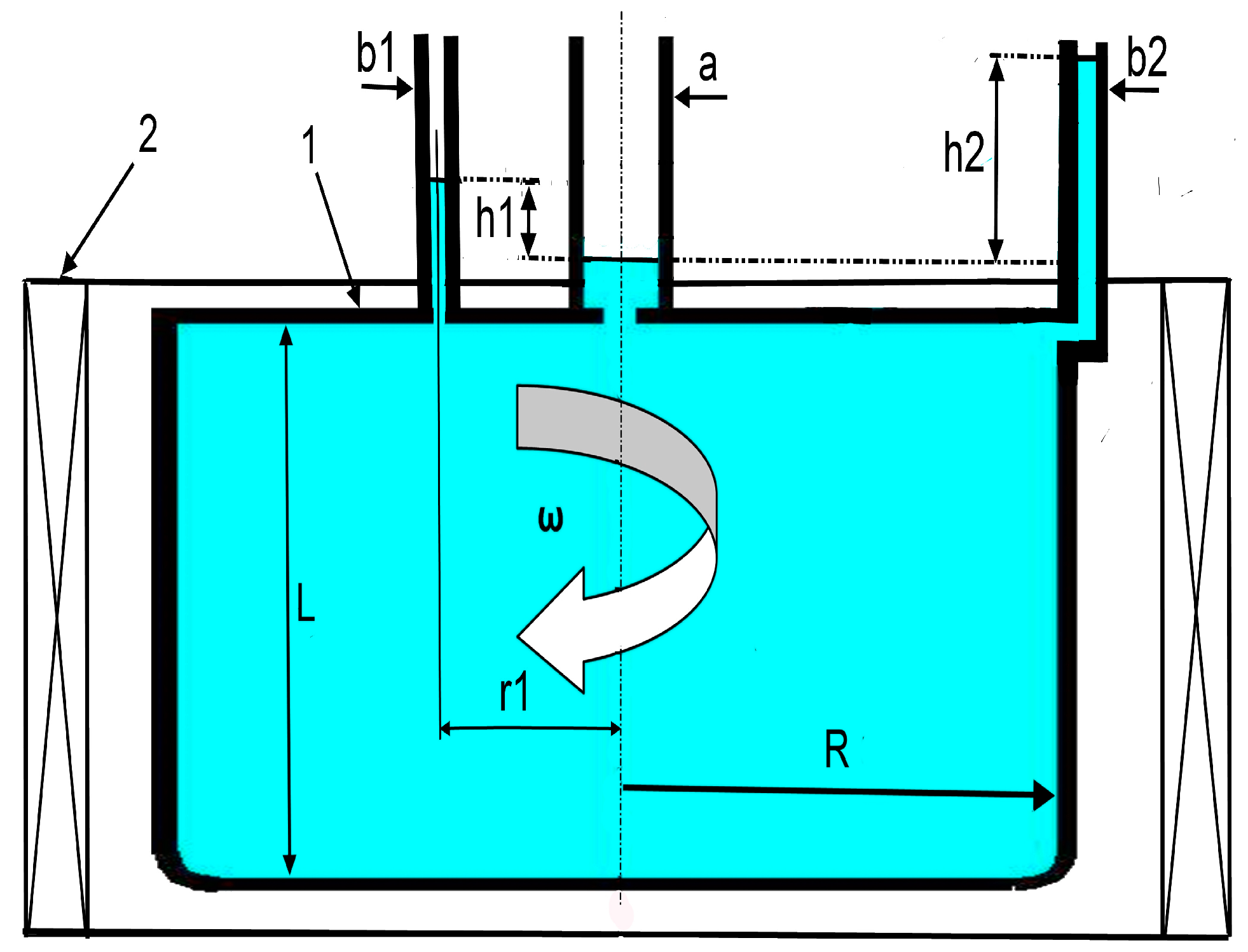
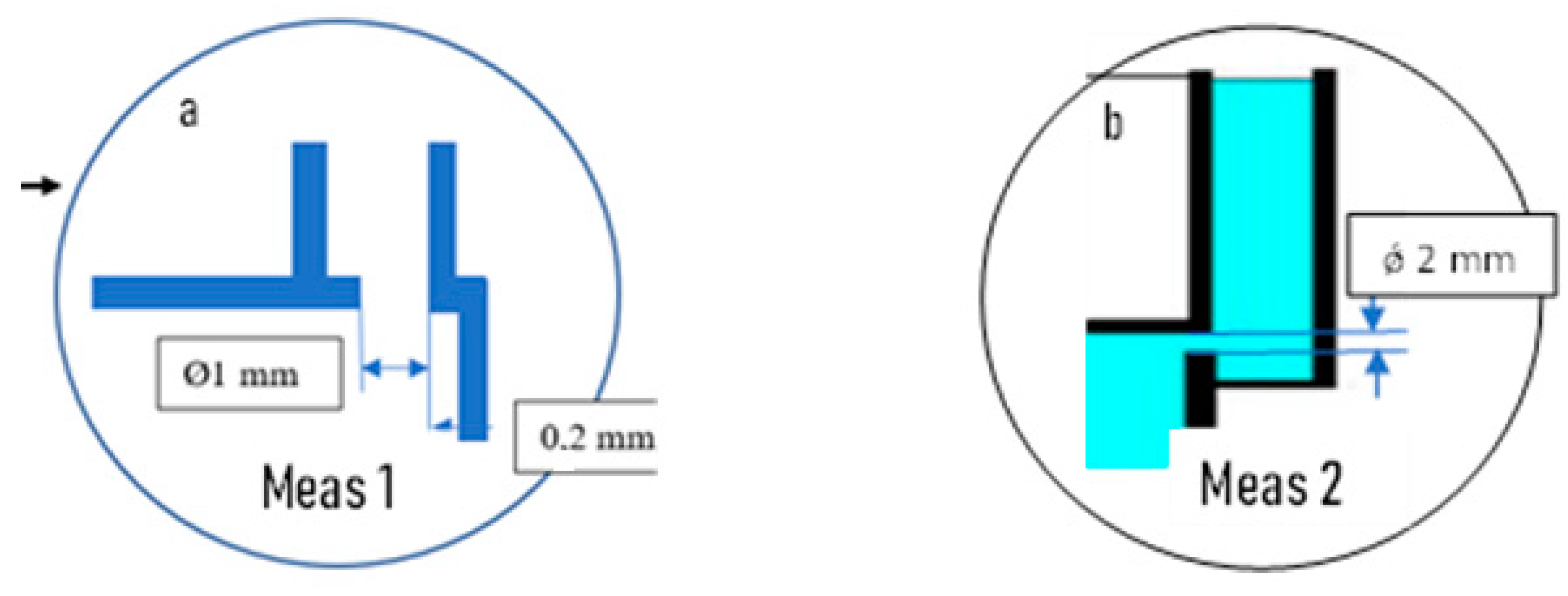
As mentioned earlier, this work aimed to give a correct dataset to check the ω(B, r) simulation. Compared to the four different measuring methods, it can be stated that the PCM method is the most useful in determining the ω(B, r) function after some minor reconstruction (see the advantage of this method). Therefore, four new TEFLON crucibles were used. The wall and the cover of the TEFLON crucible are very smooth, and the friction force is nearly zero [24]. The diameter of the crucibles was 25 mm (R = 12.5 mm), and the height was 60 mm. A sketch of the new type of crucible is shown in Figure 10. The ω(B, r) function value was measured at 5, 7.5, 10, and 12.5 mm from the axis. Holes were made in the axes (Figure 10“a” and Figure 11) in all crucibles, and one of these distances from the axis in the cover of the three crucibles (Figure 10“b1” and Figure 11a–c) and on the wall of the fourth crucible (Figure 10“b2” and Figure 11d) had a 2 mm diameter. The accuracy of the pressure measurements was 20 Pa. This accuracy was sufficient as the measured pressure was higher than 20 Pa in most cases.

The Ga75wt%In25wt% alloy was chosen because the experiments were performed at room temperature (20 ± 2 °C), where this alloy is melted. The physical parameters of the alloys are listed in

Table 1. The physical parameters of the Ga75wt%In25wt% alloy.

	Ga75In25
Melting point, °C	15.7
Density, kg/m3 (at m.p.)         ρ	6517.5
Dynamic viscosity, kg/ms        η	2.223 × 10−3
Specific electrical conductivity, MS/m     σ	3.58
Magnetic permeability, Vs/Am      μ	4π × 10−7
Penetration depth at 50 Hz, mm       δ	36

. The molten alloy “melt cylinder” height was 60 mm, so the aspect ratio was 65/25 = 2.4. The magnetic field induction was a maximum of 95 mT, the pole number of the three-phase inductor was two, and the frequency of its power-supply voltage was 50 Hz.

4. Results

Earlier [32,33], the pressure at the wall was measured across a hole in the cover of the crucible near the wall (Figure 12a). Because it revealed the suspicion that, precisely at the wall, the angular velocity (and, thus, the measurable pressure) differs from the actual value, in this work, the hole was made on the crucible wall (Figure 12b), which was also carried out in [6]. The results of the two different measuring methods are compared in Figure 13 and

Table 2. The ω value measured using two different methods at the crucible’s wall.

r = 12.5 mm
Meas 1		Meas 2
B [mT]	ω [1/s]	B [mT]	ω [1/s]
0	0	0	0
4	6.3846676	14.66	30.4
7.7	13.08333	30.77	64.9
14.7	30.458	44.23	96.87
22.5	48.14667	75.90	149.5
30.8	64.998	88.99	169.1
37.4	82.16333	-	-
44.2	96.81667	-	-
51.6	111.784	-	-
57.7	125.286	-	-
67.3	136.904	-	-
75.9	149.5687	-	-
81.8	161.1867	-	-
89	169.1413	-	-

. There is no difference between them.

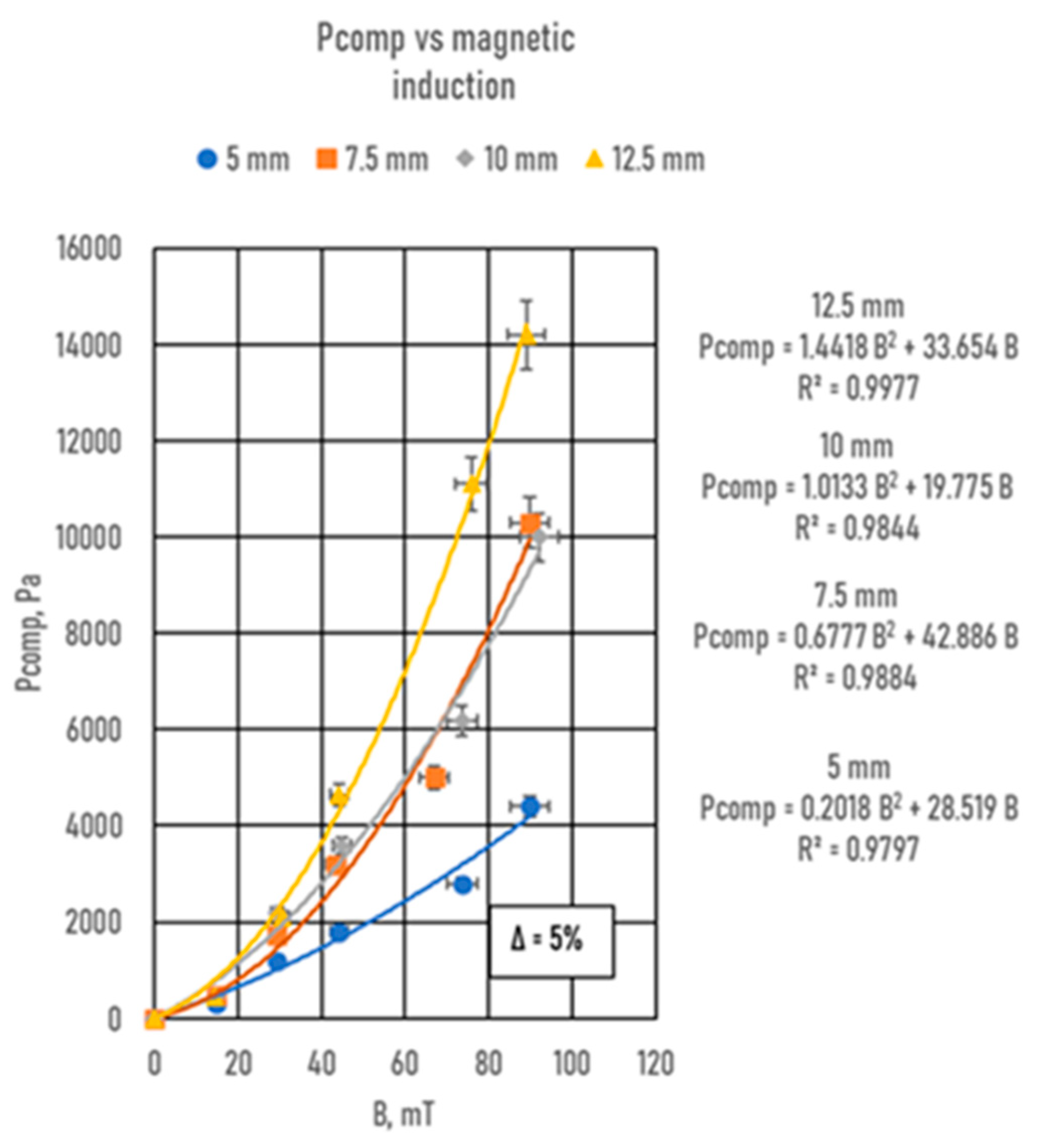
Figure 14 and

Table 3. The measured p_comp at four radiuses.

5 mm		7.5 mm		10 mm		12.5 mm
B [mT]	pcomp [Pa]	B [mT]	pcomp [Pa]	B [mT]	pcomp [Pa]	B [mT]	pcomp [Pa]
0	0	0	0	0	0	0	0
14.7	320	14.72	480	14.7	440	14.66	460
29.4	1200	29.44	1740	29.4	2200	30.77	2100
44.2	1800	43.42	3200	44.9	3580	44.23	4650
73.6	2800	66.98	5000	7.6	6180	75.9	11,100
89.8	4400	89.79	10,300	92	10,000	88.99	14,200

show the measured p_comp as a function of magnetic induction at the four different radiuses. A quadratic equation can well describe the measured values. The measuring error (Δ) is less than 5%.

Using Equations (4) and (5), the azimuthal and angular velocities (v and ω) were calculated from p_comp (Figure 15a,b and

Table 4. Calculated azimuthal and angular velocities from measured p_comp.

r, mm	Magnetic induction, B, mT					r, mm	Magnetic Induction, B, mT
	15	30	45	73	90		15	30	45	73	90
Measured Angular Velocity, ω, rad/s						Measured Azimuthal Velocity, v, mm/s
0	85.46	158.69	187.93	218	270	0	0	0	0	0	0
5	63.4	122.9	150.5	181	235	5	427.3	793.45	939.65	1090	1350
7.5	51.8	98.6	134	167	210	7.5	388.5	739.5	1005	1252.5	1575
10	37.2	83.2	106.2	139	177	10	372	832	1062	1390	1770
12.5	30.4	64.9	96.87	119	169	12.5	380	811.25	1210.875	1487.5	2112.5

). The azimuthal velocity is the highest at 12.5 mm (at the crucible wall), while it is the smallest at 5 mm, and at 7.5 and 10 mm, it is practically the same. Of course, at 0 mm, it is definitely zero. The ω(B) is approximately a straight line until 30 mT, similar to the results in [21], where the authors investigated the effect of RMF on the ω value in the case of mercury by the B-type turbine.

Because the ω(r) function is needed for the solidification simulation, based on Table 4, the azimuthal and angular velocities are shown as functions of the radius in Figure 16a,b. It can be well seen that the azimuthal and angular velocities significantly change along the radius. From the centre to the wall, the azimuthal velocity increases, and the angular velocity decreases. The theory of the flow of the liquid phase postulates that the flow velocity (in this case, the azimuthal velocity) is zero; implicitly, the angular velocity is also zero. In contrast to the theory, the measured p_comp is not zero; consequently, the azimuthal and the angular velocities also do not equal zero.

5. Discussion

5.1. An Explanation of the Changes in the Measured Angular and Azimuthal Velocity along the Radius

As mentioned earlier, in a rotating molten alloy, the angular velocity (ω) is constant as a function of the radius (r); if the magnetic induction is constant along the radius, the liquid’s viscosity produces the friction force in the molten alloy (F_fr), and the wall friction (FW) can be negligible. In this case, the free surface of the molten alloy is a paraboloid. The viscosity of the molten alloys and the wall roughness of the crucible could not be negligible, so the angular velocity changes in the rotated melt along the radius. In two earlier papers, we showed the effect of magnetic induction on the angular velocity of the melt in the case of a crucible with smooth [32] and rough [33] walls (wall friction) on the angular velocity. The angular velocity was determined using the Pressure Compensation Method (PCM) near the wall of the crucible (r ≈ R, where R is the radius of the crucible). As can be well seen from our measured data, the angular velocity decreases from the centre to the crucible wall (Figure 16). The explanation for this phenomenon is below.

Suppose a melt cylinder with electrical conductivity is placed in a rotating magnetic field with an angular velocity ω₀. In that case, if a crucible is made of electrically insulating material (i.e., TEFLON), the melting cylinder will begin to rotate. The force that produces the rotation (Lorenz force, F_.L.) is created by the interaction of the rotating magnetic field with the eddy current in the melt cylinder. When switching on the rotating magnetic field (t = 0), the angular velocity is zero (ω = 0) for all circles of the radius, R, of the melting cylinder. Thus, at the moment, t = +0 for each part of the melting cylinder on the radius, r, and F_.L. (start) is applied perpendicular to the radius.

$${\mathrm{F}}_{\mathrm{L}}\left(\mathrm{s}\mathrm{t}\mathrm{a}\mathrm{r}\mathrm{t}\right)=(1/2)\mathsf{\sigma }{\mathrm{B}}^2\mathrm{r}{\mathsf{\omega }}_0$$

(7)

where σ and B are the electrical conductivity and the magnetic induction of the inductor, respectively. It should be mentioned that Equation (1) gives an exact value if the height of the melting cylinder is H = ∞. Its radius, R, is insignificantly smaller than the penetration depth δ, i.e., R <<<< δ = [2/(ω₀σμ)]^0.5, where μ is the magnetic permeability. However, a good approximation can be used if H > 4R (in this case, 60/12.5 = 5) and 2R < δ. The force, F_.L. (start), creates a torque on the melt cylinder. It begins to rotate at an angular velocity ω, so for a rotating melt cylinder, the penetration depth will change as follows:

$$\mathsf{\delta }={[2/(({\omega }_0-\mathsf{\omega })\mathsf{\sigma }\mathsf{\mu }\left)\right]}^{0.5}$$

(8)

The angular velocity ω depends on many parameters: the aspect ratio of the melt-cylinder (L/R), the roughness of the sample holder wall (W.R.), the physical parameters of the melt (σ, μ, η), the penetration depth of the melt (δ), the value of the applied magnetic induction (B), and the radius of the given location (r). We only investigated the effect of the B and the r on the ω, while the others were constant. The value of the Lorentz force acting on the melting cylinder brought into rotation changes due to the rotation of the melting cylinder, and it begins to decrease with an increasing ω:

$${\mathrm{F}}_{\mathrm{L}}\left(\mathsf{\omega }\right)=(1/2)\mathsf{\sigma }{\mathrm{B}}^2\mathrm{r}\left[{\mathsf{\omega }}_0-\mathsf{\omega }\left(\mathrm{B},\mathrm{r}\right)\right]={\mathrm{K}}_1{\mathrm{B}}^2\mathrm{r}\left[{\mathsf{\omega }}_0-\mathsf{\omega }\left(\mathrm{B},\mathrm{r}\right)\right]$$

(9)

The F_fr consists of two parts: F_υ induced by the kinematical viscosity, η, and the wall friction, F_η. As the crucible material was TEFLON, the F_.W. was small [25] and only affected the crucible wall. So, inside the crucible,

$${\mathrm{F}}_{\mathrm{f}\mathrm{r}}={\mathrm{F}}_{\mathsf{\eta }}=\mathrm{A}\mathsf{\eta }\left(\frac{\mathrm{d}\mathrm{v}}{\mathrm{d}\mathrm{r}}\right)=2\mathsf{\pi }\mathrm{r}\mathsf{\eta }\left(\frac{\mathrm{r}\mathrm{d}\mathsf{\omega }}{\mathrm{d}\mathrm{r}}\right)=2\mathsf{\pi }{\mathrm{r}}^2\mathsf{\eta }\left(\frac{\mathrm{d}\mathsf{\omega }}{\mathrm{d}\mathrm{r}}\right)\approx 2\mathsf{\pi }{\mathrm{r}}^2\mathsf{\eta }\left(\frac{\mathsf{\omega }}{\mathrm{R}}\right)={\mathrm{K}}_2{\mathrm{r}}^2\mathsf{\omega }$$

(10)

When the inductor is switched on, the angular velocity ω increases, and then the F_.L. decreases from the F_.L. (start), and the F_fr increases until the equilibrium between the friction force (F_fr) in the melted Ga75In25 alloy and the Lorentz force (F_.L.) is reached (red and blue points in Figure 17):

$${\mathrm{F}}_{\mathrm{L}}\left(\mathsf{\omega }\left(\mathrm{s}\mathrm{t}\right)\right)={\mathrm{F}}_{\mathrm{f}\mathrm{r}}\left(\mathsf{\omega }\right(\mathrm{s}\mathrm{t}\left)\right)$$

(11)

The ω(st) will be the maximum (stationer) angular velocity at the radius, r. It can be seen from Figure 17 that at a higher radius (r₂), this maximum ω(st) is lower than at the smaller one (r₁). By using Equations (9) and (10), we can obtain the following:

$${\mathrm{K}}_1{\mathrm{B}}^2\mathrm{r}\left[{\mathsf{\omega }}_0-\mathsf{\omega }\left(\mathrm{B},\mathrm{r}\right)\right]={\mathrm{K}}_2{\mathrm{r}}^2\mathsf{\omega }$$

(12)

By rearranging Equation (12), we obtain

$${\mathrm{K}}_1{\mathrm{B}}^2\mathrm{r}{\mathsf{\omega }}_0={[\mathrm{K}}_1{\mathrm{B}}^2+{\mathrm{K}}_2\mathrm{r}]\mathrm{r}\mathsf{\omega }$$

(13)

And, finally,

$${\mathrm{K}}_1{\mathrm{B}}^2{\mathsf{\omega }}_0/{[\mathrm{K}}_1{\mathrm{B}}^2+{\mathrm{K}}_2\mathrm{r}]={\mathrm{B}}^2{\mathsf{\omega }}_0/[{\mathrm{B}}^2+\mathrm{K}\mathrm{r}]=\mathsf{\omega }(\mathrm{s}\mathrm{t})$$

(14)

$$\mathrm{K}=\mathrm{K}2/\mathrm{K}1=4\mathsf{\pi }\mathsf{\eta }/\mathrm{R}\mathsf{\sigma }$$

(15)

The value of K can be determined theoretically with Equation (15), but because $\left(\frac{\mathrm{d}\mathsf{\omega }}{\mathrm{d}\mathrm{r}}\right)\approx \mathsf{\omega }/\mathrm{R}$ is an approximation, K = 300 was determined by regression.

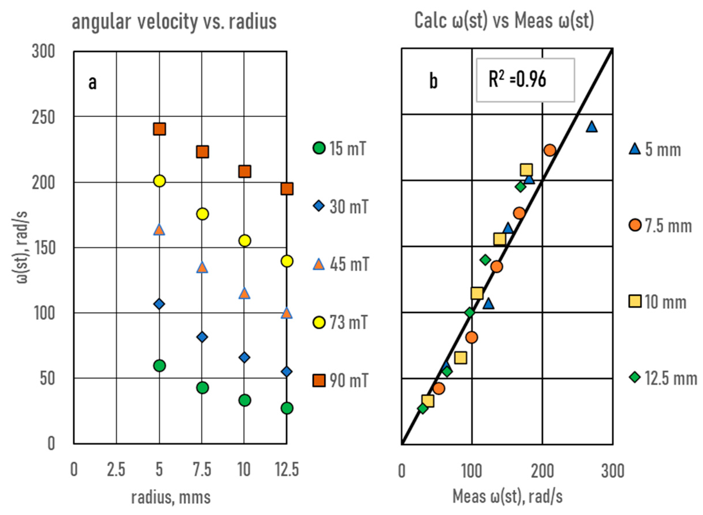
Figure 18a shows the calculated ω(st) at five magnetic inductions as a function of the radius; in Figure 18b, the measured and calculated ω(st) values are compared. As R² = 0.96, the fitting is good enough to prove the theory for the evolution of the stationary angular velocity. Based on this figure, it can be stated that the angular velocity changes along the radius; the maximum and the minimum are near the centre and at the wall, respectively.

Consequently, the angular velocity measured in [32,33] close to the crucible wall has only given information about the minimum angular velocity as a function of magnetic induction B and the crucible’s radius, R.

According to the theory, the velocity of the flowing melt (here, the azimuthal velocity) on the crucible wall is zero, so the angular velocity must be zero, too. The p_comp measured at the crucible wall (or very close to it) is not zero, so the angular velocity is also not zero.

5.2. Direct Determination of ω(B,r) Function from Measured Values of ω

We must mention that the model and the calculation shown before are only valid for laminar flow, and not for turbulent flow, and it cannot consider the change in the magnetic induction along the radius because the penetration distance decreases with the increasing angular velocity. So, we worked out another method for calculating the angular velocity as a function of the magnetic induction and the radius. Because this method is based on the direct processing of measured data, it is usable at a high magnetic induction, which causes turbulent flow, and the change in the magnetic induction along the radius can be considered. The azimuthal and angular velocities vs. the radius and the magnetic induction (ω(B,r) function are interesting for the simulation. So, based on the measured values of ω, it was constructed as detailed below.

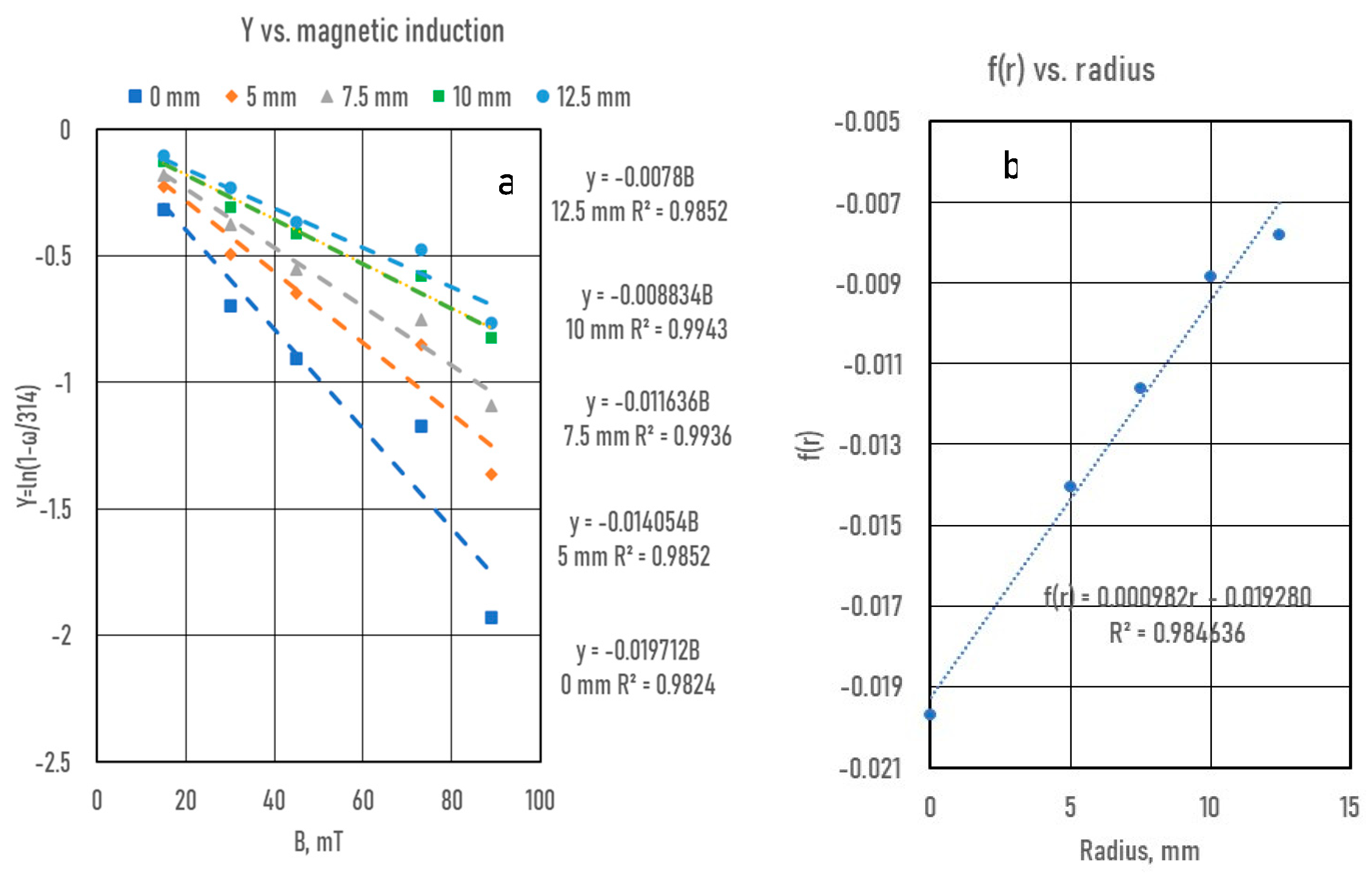
The following function estimated the ω(B, r) functions:

$$\mathsf{\omega }\left(\mathrm{B},\mathrm{r}\right)={\mathsf{\omega }}_{\mathrm{m}\mathrm{a}\mathrm{x}}\left(1-\exp \left[\mathrm{f}\right(\mathrm{r}\right)\mathrm{B}\left]\right)$$

(16)

We rearranged this equation as follows:

$$\mathrm{Y}=\mathrm{l}\mathrm{n}(1-\mathsf{\omega }\left(\mathrm{B},\mathrm{r}\right)/{\mathsf{\omega }}_{\mathrm{m}\mathrm{a}\mathrm{x}})=\mathrm{f}\left(\mathrm{r}\right)\mathrm{B}$$

(17)

In Figure 19a, Y is shown as a function of B at five different radiuses. If the R² > 0.98, then the error is acceptable. The slope (f(r)) of the Y functions can be seen in Figure 19b as a function of r:

$$\mathrm{f}\left(\mathrm{r}\right)=9.82 {10}^{-4}\mathrm{r}+1.928 {10}^{-2}$$

(18)

If the R² > 0.98, then the fit is also acceptable.

Finally,

$$\mathsf{\omega }\left(\mathrm{B},\mathrm{r}\right)=314\left(1-\exp [(9.82 {10}^{-4}\mathrm{r}+1.928 {10}^{-2}\right)\mathrm{B}]$$

(19)

$$\mathrm{v}=\mathsf{\omega }\mathrm{r}$$

(20)

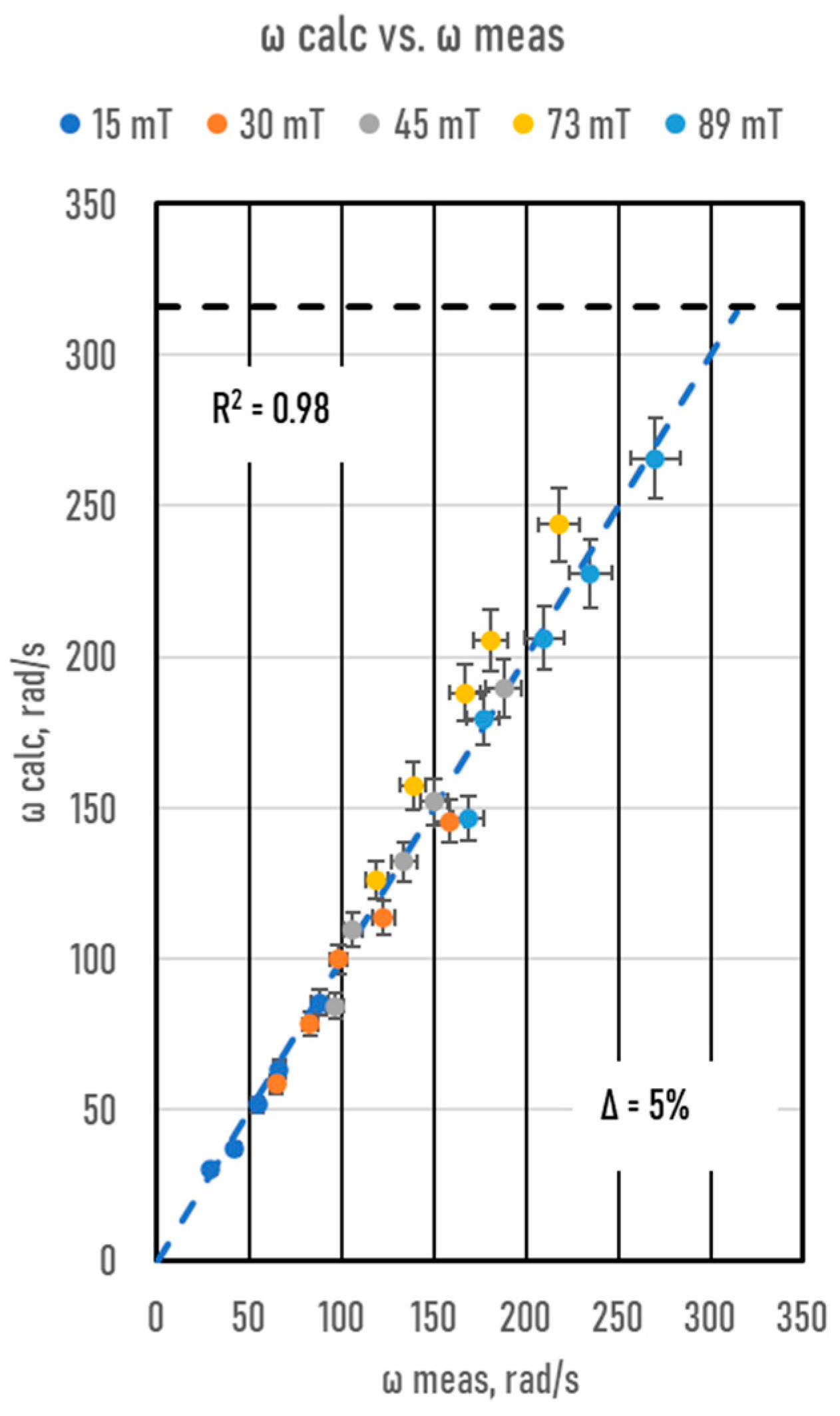
In Figure 20a,b, the measured and calculated angular and azimuthal velocities are compared as functions of the radius at the five magnetic inductions. In Figure 21, all measured and calculated angular velocities are compared. Based on these figures, it can be stated that with Equation (19), the angular velocity is calculatable with acceptable error (R² = 0.98) as a function of the radius and magnetic induction, which is usable in the simulation software.

In Figure 22, the angular and azimuthal velocities are shown in a wide range of magnetic inductions at five different radiuses. It can be seen that ω_max = 314 rad/s can be reached using about 200 mT at r = 5 mm, while at r =12.5 mm, about 800 mT is needed. It must be mentioned that the curves are verified in the range of magnetic induction between 0 and 90 mT, and from 90 to 800 mT, only the estimation is based on the measured data.

6. Conclusions

The angular velocity of the Ga75In25 melt rotated using an RMF was measured as a function of the radius in the crucible using the Pressure Compensation Method. Based on the measured ω(B, r) dataset, the following conclusions were established:

(i)

Based on a simple physical model, a calculation method was worked out for the calculation of the (ω(B, r) function:

$$\mathsf{\omega }\left(\mathrm{s}\mathrm{t}\right)={\mathrm{B}}^2{\mathsf{\omega }}_0/[{\mathrm{B}}^2+\mathrm{K}\mathrm{r}]$$

(ii)

With the simple physical model and calculation, it was proven that the angular velocity strongly depends on the radius in the crucible; the highest is at the axis, and the smallest is at the wall and continuously increases from the wall to the axis.

(iii)

The zero angular velocity given by the theory was not demonstratable when it was measured directly at the wall.

(iv)

As the simple model is valid only at laminar flow, the ω(B, r) functions were estimated based directly on the measured ω, which can correspond to the change in the magnetic induction along the radius and the effect of the turbulence of the flow by a function that can be usable in the simulations:

$$\mathsf{\omega }\left(\mathrm{B},\mathrm{r}\right)={\mathsf{\omega }}_{\mathrm{m}\mathrm{a}\mathrm{x}}\left(1-\exp \left[\mathrm{f}\right(\mathrm{r}\right)\mathrm{B}]$$

where ω_max = 314, and

$$\mathrm{f}\left(\mathrm{r}\right)=9.82 {10}^{-4}\mathrm{r}+1.928 {10}^{-2}$$

References

- Kunstreich, S. Electromagnetic stirring for continuous casting Part II. Metall. Res. Technol. 2003, 100, 1043–1061. [Google Scholar] [CrossRef]
- Stiller, J.; Koal, K.; Nagel, W.E.; Pal, J.; Cramer, A. Liquid metal flows driven by rotating and traveling magnetic fields. Eur. Phys. J. Spec. Top. 2013, 220, 111–122. [Google Scholar] [CrossRef]
- Tzavaras, A.A.; Brody, H.D. Electromagnetic Stirring and Continuous Casting—Achievements, Problems, and Goals. J. Met. 1984, 36, 31–37. [Google Scholar] [CrossRef]
- Maurya, A.; Kumar, R.; Jha, P.K. Simulation of electromagnetic field and its effect during electromagnetic stirring in continuous casting mold. J. Manuf. Process. 2020, 60, 596–607. [Google Scholar] [CrossRef]
- Yao, C.; Wang, M.; Ni, Y.; Gong, J.; Xing, L.; Zhang, H.; Bao, Y. Effects of Secondary Cooling Segment Electromagnetic Stirring on Solidification Behavior and Composition Distribution in High-Strength Steel 22MnB5. JOM 2022, 74, 4823–4830. [Google Scholar] [CrossRef]
- Sun, H.; Zhang, J. Study on the Macrosegregation Behaviour for the Bloom Continuous Casting: Model Development and Validation. Metall. Mater. Trans. B 2014, 45, 1133–1149. [Google Scholar] [CrossRef]
- Yu, H.Q.; Zhu, M.Y. Influence of electromagnetic stirring on transport phenomena in round billet continuous casting mould and macrostructure of high carbon steel billet. Ironmak. Steelmak. 2012, 39, 574–584. [Google Scholar] [CrossRef]
- Guan, R.; Ji, C.; Zhu, M. Modeling the Effect of Combined Electromagnetic Stirring Modes on Macrosegregation in Continuous Casting Blooms. Met. Mater. Trans. B 2020, 51, 1137–1153. [Google Scholar] [CrossRef]
- Fang, Q.; Zhang, H.; Wang, J.; Liu, C.; Ni, H. Effect of Electromagnetic Stirrer Position on Mold Metallurgical Behaviour in a Continuously Cast Bloom. Met. Mater. Trans. B 2020, 51, 1705–1717. [Google Scholar] [CrossRef]
- Zhang, H.; Wu, M.; Zhang, Z.; Ludwig, A.; Kharicha, A.; Rónaföldi, A.; Roósz, A.; Veres, Z.; Svéda, M. Experimental Evaluation of MHD Modelling of EMS during Continuous Casting. Metall. Mater. Trans. B 2022, 53, 2166–2181. [Google Scholar] [CrossRef]
- Sahoo, P.P.; Kumar, A.; Halder, J.; Raj, M. Optimisation of Electromagnetic Stirring in Steel Billet Caster by Using Image Processing Technique for Improvement in Billet Quality. ISIJ Int. 2009, 49, 521–528. [Google Scholar] [CrossRef]
- Willers, B.; Eckert, S.; Nikrityuk, P.; Räbiger, D.; Dong, J.; Eckert, K.; Gerbeth, G. Efficient Melt Stirring Using Pulse Sequences of a Rotating Magnetic Field: Part II. Application to Solidification of Al-Si Alloys. Met. Mater. Trans. B 2008, 39, 304–316. [Google Scholar] [CrossRef]
- Kunstreich, S. Electromagnetic stirring for continuous casting–Part I. Metall. Res. Technol. 2003, 100, 395–408. [Google Scholar] [CrossRef]
- Scholes, A. Segregation in continuous casting. Ironmak. Steelmak. 2005, 32, 101–108. [Google Scholar] [CrossRef]
- Li, P.; Zhang, G.; Yan, P.; Tian, N.; Feng, Z. Numerical and Experimental Study on Carbon Segregation in Shaped Billet of Medium Carbon Steel with Combined Electromagnetic Stirring. Materials 2023, 16, 7464. [Google Scholar] [CrossRef]
- Aycicek, I.; Solak, N. Optimization of Macro Segregation and Equiaxed Zone in High-Carbon Steel Use in Prestressed Concrete Wire and Cord Wire Application. Metals 2023, 13, 1435. [Google Scholar] [CrossRef]
- Li, J.; Deng, B.; Yang, X.; Liang, L.; Wang, H.; Wu, T. Microstructure Control of Continuous Casting Slab of Grain Oriented Silicon. Steel. Mater. Trans. 2022, 63, 112–117. [Google Scholar] [CrossRef]
- Lu, H.-B.; Zhong, Y.-B.; Ren, Z.-M.; Ren, W.-L.; Cheng, C.-G.; Lei, Z.-S. Numerical simulation of EMS position on flow, solidification and inclusion capture in slab continuous casting. J. Iron Steel Res. Int. 2022, 29, 1807–1822. [Google Scholar] [CrossRef]
- Zappulla, M.L.; Cho, S.-M.; Koric, S.; Lee, H.-J.; Kim, S.-H.; Thomas, B.G. Multiphysics Modeling of Continuous Casting of Stainless Steel. J. Am. Acad. Dermatol. 2020, 278, 116469. [Google Scholar] [CrossRef]
- Barna, M.; Javurek, M.; Wimmer, P. Numeric Simulation of the Steel Flow in a Slab Caster with a Box-Type Electromagnetic Stirrer. Steel Res. Int. 2020, 91, 9. [Google Scholar] [CrossRef]
- Spitzer, K.-H.; Dubke, M.; Schwerdtfeger, K. Rotational Electromagnetic Stirring in Continuous Casting of Round Strands. Met. Trans. B 1986, 17, 119–131. [Google Scholar] [CrossRef]
- Gelfgat, Y.M.; Gelfgat, A.Y. Experimental and Numerical Study of Rotating Magnetic Field Driven Flow in Cylindrical Enclosures with Different Aspect Ratios. Magnetohydrodynamics 2004, 40, 147–160. [Google Scholar] [CrossRef]
- Roplekar, J.K.; Dantzig, J.A. A study of solidification with a rotating magnetic field. Int. J. Cast Met. Res. 2001, 14, 79–95. [Google Scholar] [CrossRef]
- Eckert, S.; Nikrityuk, P.A.; Räbiger, D.; Eckert, K.; Gerbeth, G. Efficient Melt Stirring Using Pulse Sequences of a Rotating Magnetic Field: Part I. Flow Field in a Liquid Metal Column. Met. Mater. Trans. B 2008, 39, 374–386. [Google Scholar] [CrossRef]
- Grants, I.; Gerbeth, G. Experimental study of non-normal nonlinear transition to turbulence in a rotating magnetic field driven flow. Phys. Fluids 2003, 15, 2803–2809. [Google Scholar] [CrossRef]
- Räbiger, D.; Eckert, S.; Gerbeth, G. Measurements of an unsteady liquid metal flow during spin-up driven by a rotating magnetic field. Exp. Fluids 2010, 48, 233–244. [Google Scholar] [CrossRef]
- Dold, P.; Benz, K. Modification of Fluid Flow and Heat Transport in Vertical Bridgman Configurations by Rotating Magnetic Fields. Cryst. Res. Technol. 1997, 38, 39–58. [Google Scholar] [CrossRef]
- Willers, B.; Barna, M.; Reiter, J.; Eckert, S. Experimental Investigations of Rotary Electromagnetic Mould Stirring in Continuous Casting Using a Cold Liquid Metal Model. ISIJ Int. 2017, 57, 468–477. [Google Scholar] [CrossRef]
- Kapusta, A.B.; Shamota, V.P. Turbulent rotating MHD flow in finite length cylindrical container. In Proceedings of the Fourth International Conference on Magnetohydrodynamic at the Dawn of the Third Millennium, Presquile de Giens, France, 18–22 September 2000; pp. 681–686. [Google Scholar]
- Gelfgat, Y.M.; Priede, J.; Sorkin, M.Z. Numerical simulations of MDD flow induced by a magnetic field in a cylindrical container of finite length. In Proceedings of the International Conference on Energy Transfer in MHD, Grenoble, France, 30 September–3 October 1991; pp. 181–186. [Google Scholar]
- Rónaföldi, A. Development and Investigation of a Solidification Facility with a Rotating Magnetic Field. Ph.D. Thesis, University of Miskolc, Miskolc, Hungary, 2008. [Google Scholar]
- Rónaföldi, A.; Roósz, A.; Veres, Z. Determination of the conditions of laminar/turbulent flow transition using pressure compensation method in the case of Ga75In25 alloy stirred by RMF. J. Cryst. Growth 2021, 564, 126078. [Google Scholar] [CrossRef]
- Roósz, A.; Rónaföldi, A.; Svéda, M.; Veres, Z. Effect of crucible wall roughness on the laminar/turbulent flow transition of the Ga75In25 alloy stirred by a rotating magnetic field. Sci. Rep. 2022, 12, 18592. [Google Scholar] [CrossRef]
- Liu, T.Y. Numerical Simulation of Electromagnetic Stirring of Rolls in Sub-Section of Ultra-Wide Slab Second Cooling Zone. Materials 2024, 17, 1038. [Google Scholar] [CrossRef]
- Liang, M.; Cho, S.-M.; Ruan, X.; Thomas, B.G. Modeling of Multiphase Flow, Superheat Dissipation, Particle Transport, and Capture in a Vertical and Bending Continuous Caster. Processes 2022, 10, 1429. [Google Scholar] [CrossRef]
Figure 1.
A sketch of the free surface of the rotating melt if h >> R (the aspect ratio is higher than 6).
Figure 2.
Glass ampulla (a) and glass “turbine” (b), “shaft + turbine blade” (b and c), and complete measuring unit (d)
Figure 3.
Picture of process of determining Rpm of molten gallium.
Figure 4.
A sketch of the measuring possibilities with the turbine blade in a bigger crucible; 1: inductor; 2: turbine blades in 3 different positions of the crucible.
Figure 5.
Sketch of turbine (version B); 1: inductor, 2: turbine blades, 3: shaft of turbine blades, 4: glass crucible, 5: fixing wheel, 6: crucible cover.
Figure 6.
Sketch of facility using conductive anemometer with its own magnetic field; 1: inductor, 2: permanent magnet, 3: ceramic tube, 4: nano-voltmeter, 5: crucible.
Figure 7.
Developing the melt level difference, Δh, in the gauges connected to the closed crucible. The melt levels before (A) and after (B) the switch on the inductor; 1: closed crucible, 2: inductors, a and b: the two gauges connected to the closed crucible, L is the height and R is the crucible’s radius.
Figure 8.
1: Closed crucible; 2: inductors; a and b: the two gauges connected to the closed crucible; c: manometer.
Figure 9.
Compensation of melt levels by pcomp pressure in gauges. 1: Closed crucible; 2: inductors; a and b: the two gauges connected to the closed crucible.
Figure 10.
A sketch of the new type of crucibles. The “a” gauge is at the centre of the crucible, the “b1” gauge is in three different positions, and the “b2” gauge is at the wall of the crucible.
Figure 11.
Four crucibles with 2 mm diameter holes. The distances from the axis are (a) 5 mm, (b) 7.5 mm, (c) 10 mm, and (d) 12.5 mm. The black and yellow arrows show the holes.
Figure 12.
A sketch of the two measuring methods. (a) The measuring hole is across the crucible’s cover; (b) the measuring hole is at the crucible’s wall.
Figure 13.
A comparison of the angular velocity measured using the two methods.
Figure 14.
The measured pcomp is a function of magnetic induction.
Figure 15.
(a) The measured azimuthal and (b) angular velocities as functions of magnetic induction.
Figure 16.
(a) The measured azimuthal and (b) angular velocities as functions of the radius.
Figure 17.
Graphical calculation of the stationary angular velocity (ω(st)) at two different radiuses.
Figure 18.
(a) The calculated ω(st) vs. the radius; (b) a comparison of the measured and calculated ω(st) values.
Figure 19.
(a) Y as a function of magnetic induction (B) at five different radiuses (r); (b) f(r) as a function of r.
Figure 20.
(a) The calculated angular velocity as a function of the radius at five magnetic inductions. (b) The calculated azimuthal velocity as a function of the radius at five magnetic inductions.
Figure 21.
Comparison of measured and calculated angular velocities.
Figure 22.
(a) The calculated angular velocity as a function of a wide range of magnetic inductions at five radiuses. (b) The calculated azimuthal velocity as a function of a wide range of magnetic inductions at five radiuses.